Semantic Role Labeling via Instance Based Learning

(1)

Semantic Role Labeling via Instance-Based Learning

Chi-San Althon Lin

Department of Computer Science Waikato University Hamilton, New Zealand [email protected]

Tony C. Smith

Department of Computer Science Waikato University Hamilton, New Zealand [email protected]

Abstract

This paper demonstrates two methods to improve the performance of instance-based learning (IBL) algorithms for the problem of Semantic Role Labeling (SRL). Two IBL algorithms are utilized: k-Nearest Neighbor (kNN), and Priority Maximum Likelihood (PML) with a modified back-off combination method. The experimental data are the WSJ23 and Brown Corpus test sets from the CoNLL-2005 Shared Task. It is shown that ap-plying the Tree-Based Predicate-Argument Recognition Algorithm (PARA) to the data as a preprocessing stage allows kNN and PML to deliver F1: 68.61 and 71.02 respectively on the WSJ23, and F1: 56.96 and 60.55 on the Brown Corpus; an increase of 8.28 in F1 measurement over the most recent pub-lished PML results for this problem (Palmer et al., 2005). Training times for IBL algorithms are very much faster than for other widely used techniques for SRL (e.g. parsing, support vector machines, perceptrons, etc); and the feature reduc-tion effects of PARA yield testing and processing speeds of around 1.0 second per sentence for kNN and 0.9 second per sentence for PML respectively, suggest-ing that IBL could be a more practical way to perform SRL for NLP applica-tions where it is employed; such as real-time Machine Translation or Automatic Speech Recognition.

1 Introduction

The proceedings from CoNLL2004 and CoNLL2005 detail a wide variety of approaches to Semantic Role Labeling (SRL). Many re-search efforts utilize machine learning (ML) ap-proaches; such as support vector machines (Mo-schitti et al., 2004; Pradhan et al., 2004), percep-trons (Carreras et al., 2004), the SNoW learning architecture (Punyakanok et al., 2004), EM-based clustering (Baldewein et al., 2004), trans-formation-based learning (Higgins, 2004), mem-ory-based learning (Kouchnir, 2004), and induc-tive learning (Surdeanu et al., 2003). This paper compares two instance-based learning ap-proaches, kNN and PML. The PML method used here utilizes a modification of the backoff lattice method used by Gildea & Jurafsky (2002) to use a set of basic features—specifically, the features employed for learning in this paper are Predicate (pr), Voice (vo), Phrase Type (pt), Dis-tance (di), Head Word (hw), Path (pa), Preposi-tion in a PP (pp), and an “Actor” heuristic.

The general approach presented here is an example of memory-based learning. Many existing SRL systems are also memory-based (Bosch et al., 2004;Kouchnir, 2004), implemented using TilMBL software (http://ilk.kub.nl/software.html) with advanced methods such as Feature Weighting, and so forth. This paper measures the performance of kNN and PML for comparison in terms of accuracy and processing speed, both against each other and against previously published results.

2 Related Work

Features

(2)

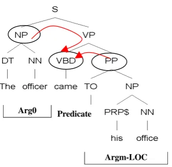
Figure 1. Illustration of path “NP↑S↓VP↓VBD” from a constituent “The officer” to the predicate “came” .

Predicate – the given predicate lemma

Voice – whether the predicate is realized as an active or passive construction (Pradhan et al., 2004, claim approximately 11% of the sentences in PropBank use a passive instantiation)

Phrase Type – the syntactic category (NP, PP, S, etc.) of the phrase corresponding to the semantic argument

Distance – the relative displacement from the predicate, measured in intervening constituents (negative if the constituent appears prior to the predicate, positive if it appears after it)

Head Word – the syntactic head of the phrase, calculated by finding the last noun of a Noun Phrase

Path – the syntactic path through the parse tree, from the parse constituent to the predicate being classified (for example, in Figure 1, the path from Arg0 – “The officer“ to the predicate “came“, is represented with the string NP↑S↓VP↓VBD” represent upward and downward movements in the tree respectively)

Preposition – the preposition of an argument in a PP, such as “during”, “at”, “with”, etc (for exam-ple, in Figure 1, the preposition for the PP with Argm-Loc label is “to”).

In addition, an actor heuristic is adopted: where an instance can be labeled as A0 (actor) only if the argument is a subject before the predicate in active voice, or if the preposition “by” appears prior to this argument but after the predicate in a passive voice sentence. For example, if there is a set of labels, A0 (subject or actor) V (active) A0 (non actor), then the latter “A0” after V is skipped and labeled to another suitable role by this heuristic; such as the label with the second highest probability for this argument according

to the PML estimate, or with the second shortest distance estimate by kNN.

2.1 k Nearest Neighbour (kNN) Algorithm

One instance-based learning algorithm is k-Nearest Neighbour (kNN), which is suitable when 1) instances can be mapped to points/classifications in n-dimensional feature dimension, 2) fewer than 20 features are utilized, and 3) training data is sufficiently abundant. One advantage of kNN is that training is very fast; one disadvantage is it is generally slow at testing. The implementation of kNN is described as following

1. Instance base:

All the training data is stored in a format similar to Bosch et al., (2004)—specifically, “Role, Predicate, Voice, Phrase type, Dis-tance, Head Word, Path”. As an example in-stance, the second argument of a predicate “take” in the training data is stored as: A0 take active NP –1 classics NP↑S↓VP↓VBD This format maps each argument to six fea-ture dimensions + one classification. 2. Distance metric (Euclidean distance) is

de-fined as:

D(xi, xj) =

√

Σ(ar(xi))-ar(xj))2

where r=1 to n (n = number of different clas-sifications), and ar(x) is the r-th feature of in-stance x. If inin-stances xi and xj are identical, then D(xi , xj )=0 otherwise D(xi , xj ) repre-sents the vector distance between xi and xj . 3. Classification function

Given a query/test instance xq to be classified, let x1, ... xk denote the k instances from the training data that are nearest to xq. The clas-sification function is

F^(xq) <- argmaxΣδ(v,f(xi))

where i =1 to k, v =1 to m (m = size of train-ing data), δ(a,b)=1 if a=b, 0 otherwise; and v denotes a semantic role for each instance of training data.

Computational complexity for kNN is linear, such that TkNN -> O( m * n ), which is propor-tional to the product of the number of features (m) and the number of training instances (n).

2.2 Priority Maximum Likelihood (PML) Estimation

Gildea & Jurafsky (2002), Gildea & Hocken-maier (2003) and Palmer et al., (2005) use a sta-tistical approach based on Maximum Likelihood method for SRL, with different backoff combina-Predicate

Arg0

[image:2.595.125.294.111.274.2]

(3)

P(r | hw, pt, pre ,pp) P(r | pt, pa, pr, pp) P(r | pt, di, vo, pr, pp)

P(r | hw, pr, pp) P(r | pt, pr, pp)

P(r | pr, pp) Local

Global

P(r | hw, pp) P(r | pt, di, vo, pp)

tion methods in which selected probabilities are combined with linear interpolation. The prob-ability estimation or Maximum Likelihood is based on the number of known features available. If the full feature set is selected the probability is calculated by

P (r | pr, vo, pt, di, hw, pa, pp) = # (r, pr, vo, pt, di, hw, pa, pp) /

# (pr, vo, pt, di, hw, pa, pp)

Gildea & Jurafsky (2002) claims “there is a trade-off between more-specific distributions, which have higher accuracy but lower coverage, and less-specific distributions, which have lower accuracy but higher coverage” and that the se-lection of feature subsets is exponential; and that selection of combinations of different feature subsets is doubly exponential, which is NP-complete. Gildea & Jurafsky (2002) propose the backoff combination in a linear interpolation for both coverage and precision. Following their lead, the research presented here uses Priority Maximum Likelihood Estimation modified from the backoff combination as follows:

P’ ( r | pr, vo, pt, di, hw, pa, pp) =

where Σiλi = 1.

Figure 2 depicts a graphic organization of the priority combination with more-specific distribu-tion toward the top, similar to Palmer et al. (2005) but adding another preposition feature. The backoff lattice is consulted to calculate probabili-ties for whichever subset of features is available to combine. As Gildea & Jurasksy (2002) state, “the less-specific distributions were used only when no data were present for any more-specific distribution. Thus, the distributions selected are arranged in a cut across the lattice representing the most-specific distributions for which data are available.”

Figure 2. Combination of Priority Estimation for PML system originated from Gildea et al., (2002)

The classification decision is made by the fol-lowing calculation for each argument in a sen-tence: argmax_r

1 .. nP(r1…n | f1,..n) This approach is described in more detail in Gildea and Jurasky (2002).

The computational complexity of PML is hard to calculate due to the many different distributions at each priority level. In Figure 2, the two calcu-lations P(r | hw, pp), and P(r | pt, di, vo, pp) be-long to the global search, while the rest bebe-long to a local search which can reduce the computa-tional complexity. Examination of the details of execution time (described in the results section of this paper) show that a plot of the execution time exhibits logarithmic characteristics, imply-ing that the computational complexity for PML is log-linear, such that TPML -> O( m * log n ) where m denotes the size of features and n de-notes the size of training data.

2.3 Predicate-Argument Recognition Algo-rithm (PARA)

Lin & Smith (2005; 2006) describe a tree-based predicate-argument recognition algorithm (PARA). PARA simply finds all boundaries for given predicates by browsing input parse-trees, such as given by Charniak’s parser or hand-corrected parses. There are three major types of phrases including given predicates, which are VP, NP, and PP. Boundaries can be recognized within boundary areas or from the top levels of clauses (as in Xue & Palmer, 2004). Figure 3 shows the basic algorithm of PARA, and more details can be found in Lin & Smith (2006). The best state-of-the-art ML technique using the same syntactic information (Moschitti, 2005) only just outperforms a preliminary version of PARA in F1 from 80.72 to 81.52 for boundary recognition tasks. ButPARA is much faster than all other existing techniques, and is therefore used for preprocessing in this study to minimize query time when applying instance-based learn-ing to SRL. The computational complexity of PARA is constant.

3 System Architecture

(4)

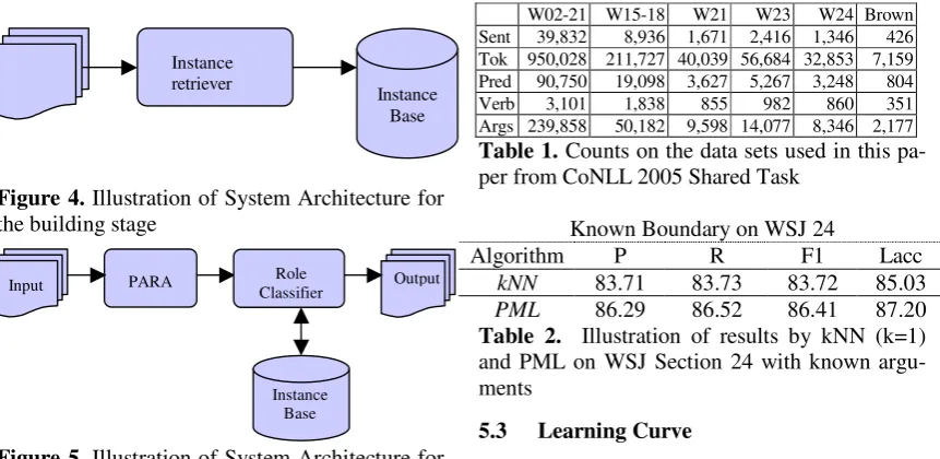
Phrase Type (pt), Path (pa), Distance (di), Head Word (hw), Preposition in a PP (pp) }. Figure 5 characterizes the testing stage, where new in-stances are classified by matching their feature representation to all instances in memory in or-der to find the most similar instances. There are two tasks during the testing stage: Argument Identification (or Boundary recognition) per-formed by PARA, and Argument Classification (or Role Labeling) performed using either kNN or PML. This approach is thus a “lazy learning” strategy applied to SRL because no calculations occur during the building stage.

4 Data, Evaluation, and Parsers

The research outlined here uses the dataset re-leased by the CoNLL-05 Shared Task (http://www.lsi.upc.edu/~srlconll/soft.html). It includes several Wall Street Journal sections with parse-trees from both Charniak’s (2000) parser and Collins’ (1999) parser. These sections are also part of the PropBank corpus (http://www.cis.upenn.edu/~treebank). WSJ

sec-tions 20 and 21 (with Charniak’s parses) were used as test data. PARA operates directly on the parse tree. Evaluation is carried out using preci-sion, recall and F1 measures of assignment-accuracy of predicated arguments. Precision (p) is the proportion of arguments predicated by the system that are correct. Recall (r) is the propor-tion of correct arguments in the dataset that are predicated by the system.

Finally, the F1 measure computes the harmonic mean of precision and recall, such that F1 =2*p*r / (p+r), and is the most commonly used primary measure when comparing different SRL systems. For consistency, the performance of PARA for boundary recognition is tested using the official evaluation script from CoNLL 2005, srl-eval.pl (http://www.lsi.upc.edu/~srlconll/soft.html) in all experiments presented in this paper. Related sta-tistics of training data and testing data are out-lined in Table 1. The average number of predi-cates in a sentence for WSJ02-21 is 2.27, and each predicate comes with an average of 2.64 arguments.

Create_Boundary(predicate, tree)

If the phrase type of the predicate == VP

- find the boundary area ( the closest S clause) - find NP before predicate

- If there is no NP, then find the closest NP from Ancestors. - find if WHNP in it’s siblings of the boundary area,

if found // for what, which, that , who,…

- if the word of the first WP’s family is “what” then - add WHNP to boundary list

else // not what, such as who which,… - find the closest NP from Ancestors - add the NP to the boundary list and add this WHNP to boundary list as reference of NP

- add valid boundaries of the rest of constituents to boundary list.

If phrase type of the predicate ==NP

- find the boundary area ( the NP clause)

- find RB(POS) before predicate and add to boundary list. - Add this predicate to boundary list.

- Add the rest of word group after the predicate and before the end of the NP clause as a whole boundary to boundary list.

If phrase type of the predicate ==PP

- find the boundary area ( the PP clause)

- find the closet NP from Ancestors if the lemma of the predicate is “include”, and add this NP to boundary list.(special for PropBank)

- Add this predicate to boundary list. -

Add the rest of children of this predicate to boundary list or add one closest NP outside the boundary area to boundary list if there is no child after this predicate.

(5)

Figure 4. Illustration of System Architecture for the building stage

Figure 5. Illustration of System Architecture for the testing stage

5 Experiments and Results

Experimental results were obtained for part of the Brown corpus (the part provided by CoNLL-2005) and for Wall Street Journal (WSJ) Sections 21, 23, and 24 using different training data sets (WSJ 21, WSJ 15 to 18, and WSJ 02 to 21) shown in Table 1. There are two tasks, Role classification with known arguments as input, and Boundary recognition & Role classification with gold (hand-corrected) parses or auto (Charniak’s) parses. In addition, execution speed, the learning curve, and some further results for exploration of kNN and PML are also included below.

5.1 WSJ 24 with known arguments

Table 2 shows the results from kNN and PML with known boundaries/arguments (i.e. the sys-tems are given the correct arguments for role classification). All training datasets (WSJ02-21) include Charniak’s parse trees. The table shows that PML achieves F1: 2.69 better than kNN.

5.2 Features & Heuristic on WSJ 24 with known arguments

Table 3 shows the contribution of each feature and the actor heuristic by excluding one feature or heuristic. It indicates that Head Word, Prepo-sition, and Distance are the three features that contribute most to system accuracy, and the addi-tional Actor heuristic is fourth. Path, Phrase type and Voice are the three features contibuting the least for both classification algorithms.

W02-21 W15-18 W21 W23 W24 Brown Sent 39,832 8,936 1,671 2,416 1,346 426 Tok 950,028 211,727 40,039 56,684 32,853 7,159 Pred 90,750 19,098 3,627 5,267 3,248 804 Verb 3,101 1,838 855 982 860 351 Args 239,858 50,182 9,598 14,077 8,346 2,177

Table 1. Counts on the data sets used in this pa-per from CoNLL 2005 Shared Task

Known Boundary on WSJ 24

Algorithm P R F1 Lacc

kNN 83.71 83.73 83.72 85.03

PML 86.29 86.52 86.41 87.20 Table 2. Illustration of results by kNN (k=1) and PML on WSJ Section 24 with known argu-ments

5.3 Learning Curve

Table 4 shows that performance improves as more training data is provided; and that PML outperforms kNN by about F1:2.8 on average for WSJ 24 for the three different training sets, mainly because the backoff lattice improves both recall and precision. The table shows that it is not always beneficial to include all features for labeling all roles. While P(r | hw, pt, pre, pp) is mainly for adjunctive roles (e.g. AM-TMP), P(r | pt, di, vo, pr, pp) is mainly for core roles (e.g. A0).

5.4 Performance of Execution Time

Building (or training) timeis about 2.5 minutes for both PML and kNN, whereas it takes any-where from about 10 hours to 60 hours for other ML-based architectures (according to the data presented by McCracken http://www.lsi.upc.es/ ~srlconll/st05/slides/mccracken.pdf). Table 5 shows average execution time (in seconds) per sentence for the two algorithms. PML runs faster than kNN when all 20 training datasets are used (i.e. WSJ 02 to 21). A graphic illustration of execution speed is shown in Figure 6. The simulation formulas for PML and kNN are “y = 0.1734Ln(x) - 0.9046” and “y = 2.441*10-5 x + 0.0129” respectively. “x” denotes numbers of training sentences, and “y” denotes second per sentence related to “x” training sentences. The execution time for PML is about 8 times longer than kNN for 1.7k training sentences, but PML ultimately runs faster than kNN on all 39.8K training sentences (and, extrapolating from the graph in Figure 6, on any larger datasets). Thus PML seems generally more suitable for large training data.

Input Instance retriever

Instance Base

Input PARA

Instance Base Role

[image:5.595.107.538.95.305.2]

(6)

Training sets KNN PML

WSJ 21 0.050 0.396

WSJ 15 - 18 0.241 0.687

WSJ 02 - 21 1.000 0.941

Table 5. Illustration of results for execution time by kNN and PML on WSJ 24 with known arguments

0 0.1 0.2 0.3 0.4 0.5 0.6 0.7 0.8

0.91

1.1

Figure 6. Curve of execution time for kNN (k=1) and PML on WSJ 24 with known arguments

5.5 WSJ 24 with Gold parses and PARA

Table 6 shows performance for both systems when gold (hand-corrected) parses are supplied and PARA preprocessing is employed. Com-pared to the results in Table 4, the performance on the combined training sets (WSJ 02 to 21) drops F1:9.24 and Lacc (label accuracy):2.4 for kNN; and drops F1:8.02 and Lacc:0.66 for PML respectively. This may indicate that PML is more error tolerant in labeling accuracy. How-ever, both systems perform worse due largely to an idiosyncratic problem in the PARA-preprocessor when dealing with hand-corrected parses—ultimately due to a particular parsing error.

5.6 WSJ 24 with Charniak’s parses and PARA

Table 7 shows the performance of both systems using auto-parsing (i.e. Charniak’s parser) and PARA argument recognition. Compared to the results in Table 4, the performance on all training sets (WSJ 02 to 21) drops F1:17.25 and Lacc:0.65 for kNN, and F1:16.78 and Lacc:-0.78 (i.e. increasing Lacc) for PML respectively. Both systems drop a lot in F1 due to errors caused by the auto-parser (in particular errors relating to punctuation), whose effects are subse-quently exacerbated by PARA. Even so, the la-bel accuracy (Lacc) is more or less similar be-cause the training dataset are parsed by Charniak’s parser instead of gold parses.

5.7 WSJ 23 with Charniak’s parses and PARA

Table 8 shows the results for WSJ 23, where the performance of PML exceeds kNN by about F1:3.8. WSJ 23 is used as a comparison dataset in SRL. More comparisons with other systems are shown in Table 12.

5.8 Brown corpus with Charniak’s parses and PARA

Table 9 shows the results when moving to a dif-ferent language domain—the Brown corpus. Both systems drop a lot in F1 . Compared to WSJ 23, MPL drops 10.47 in F1 and kNN, 11.65 in F1. These drops are caused partially by PARA, and partially by classifiers. PARA in Lin & Smith (2006) drops about 3.1 in F1 when moving to the Brown Corpus; but more research is required to uncover the cause.

5.9 Further results on kNN with all training data

Table 10 shows different results for various val-ues of k in kNN. Both systems, GP (gold-parse) & PARA and CP (Charniak’s parse) & PARA, perform best (as measured by F1) when K is set as one. But when the system is labeling a known argument, selection of k=5 is better in terms of both F1 and Label accuracy (Lacc).

5.10 Further results on PML with all train-ing data

Table 11 shows results for PML with different methods of calculating probabilities. “L+G” means the basic probability distribution (from Figure 2). “L only” and “G only” mean all prob-ability is calculated only as either “local” or “global”, respectively. “L>>G” means that probabilities are calculated globally only when the local probability is zero. “L only” is the fast-est approach, and “G only” the slowfast-est (about five seconds per sentence). Both are poor in per-formance. “L+G” has the best result and “L>>G” is rated as intermediate in performance and execution time.

5.11 Comparison with other systems

(7)

first row. The basic kNN in the fourth row, trained by four datasets (WSJ 15 to 18 in CoNLL 2004) for the RL” task (to label arguments by giving the known arguments) on the test data WSJ 21, increases F1:6.68 compared to the result of Kouchnir (2004) in the third row. Execution time for our own re-implementation of Palmer (2005) is about 3.785 sec per sentence. Instead of calculating each node in a parse tree like the Palmer (2005) model, PARA+PML can only fo-cus on essential nodes from the output of PARA,

which helps to reduce the execution time as 0.941 second per sentence. Execution time by Palmer (2005) is about 4 times longer than PARA+PML on the same machine (n.b. execu-tion times are for a computer running Linux on a P4 2.6GHz CPU with 1G MBRAM).

More details from different systems and combi-nations of systems are described in the proceed-ings of CoNLL-2005.

kNN k=1 PML

P R F1 P R F1

ALL 83.71 83.73 83.72 86.29 86.52 86.41

- Voice 81.69 81.60 81.64 85.64 85.90 85.77

- Phrase Type 82.79 82.79 82.79 85.68 85.96 85.82

- Distance 76.53 76.42 76.47 83.76 83.97 83.86

- Head Word 78.26 78.05 78.15 81.84 81.96 81.90

- Path 83.67 83.63 83.65 85.44 85.72 85.58

- Preposition 79.40 79.29 79.33 82.02 82.12 82.07

- Actor 80.38 80.64 80.51 84.74 85.01 84.81

Table 3. Illustration of contribution for each feature and the Actor heuristic by kNN (k=1) and PML on WSJ 24 with known arguments

kNN k=1 PML

Training sets P R F1 Lacc P R F1 Lacc

WSJ 21 76.76 77.02 76.89 78.03 79.20 79.26 79.23 80.40

WSJ 15 - 18 80.40 80.18 80.29 81.85 83.61 83.70 83.66 84.61

WSJ 02 - 21 83.71 83.73 83.72 85.03 86.29 86.52 86.41 87.20

Table 4. Illustration of results with different training datasets by kNN (k=1) and PML on WSJ 24 with known arguments

kNN k=1 PML

WSJ 21 67.96 67.90 67.93 75.61 70.51 70.57 70.54 78.17

WSJ 15 - 18 72.42 72.25 72.34 80.66 75.64 75.62 75.63 83.55

WSJ 02 - 21 74.48 74.48 74.48 82.63 78.39 78.40 78.39 86.54

Table 6. Illustration of results with different training datasets by kNN (k=1) and PML on WSJ 24 with gold (Hand corrected) parses and PARA

kNN k=1 PML

WSJ 21 61.05 60.90 60.98 77.45 63.75 63.43 63.59 80.70

WSJ 15 - 18 64.66 64.11 64.38 82.13 67.55 67.15 67.35 85.23

WSJ 02 - 21 66.62 66.32 66.47 84.38 69.81 69.45 69.63 87.98

Table 7. Illustration of results with different training datasets by kNN (k=1) and PML on WSJ 24 with Charniak’s parses and PARA

kNN k=1 PML

WSJ 21 62.87 62.55 62.71 78.85 64.94 64.49 64.71 81.31

WSJ 15 - 18 66.66 65.96 66.31 83.60 69.05 68.52 68.79 86.14

WSJ 02 - 21 68.92 68.31 68.61 86.20 71.24 70.79 71.02 88.77

(8)

kNN k=1 PML

WSJ 21 52.56 51.40 51.97 67.70 55.17 53.88 54.52 70.15

WSJ 15 - 18 55.58 54.20 54.88 71.56 59.10 57.56 58.32 75.53

WSJ 02 - 21 57.71 56.22 56.96 74.14 61.26 59.85 60.55 78.26

Table 9. Illustration of results with different training datasets by kNN (k=1) and PML on Brown Cor-pus with Charniak’s parses and PARA

Known boundary GP & PARA CP & PARA

K F1 Lacc F1 Lacc F1 Lacc

1 83.72 85.03 74.48 82.63 66.47 84.38

3 83.67 85.13 74.33 82.70 65.94 84.03

5 83.89 85.16 74.14 82.28 65.89 83.81

7 83.27 84.66 73.43 81.59 65.52 83.54

9 82.86 84.25 73.00 81.22 65.13 82.99

Table 10. Illustration of results by kNN with different K values on WSJ 24 with known arguments, Gold (Hand-corrected) parses & PARA and Charniak’s parses & PARA

Known boundary on WSJ 24

Method P R F1 Lacc T (Sec/Sen)

L+G 86.29 86.52 86.41 87.20 0.941

L only 80.78 80.73 80.76 81.70 0.027

G only 75.60 76.35 75.97 77.52 5.094

L>>G 82.44 82.42 82.43 83.29 0.128

Table 11. Illustration of results by PML with different methods on WSJ 24 with known arguments

System Train Test Tasks P R F1 Lacc T

Palmer (2005) W02-21 W23 BR+RL 68.60 57.80 62.74 81.70 3.785

PARA+PML W02-21 W23 BR+RL 71.24 70.79 71.02 88.77 0.941

Kouchnir (2004) W15-18 W21 RL 75.71 74.60 75.15

kNN W15-18 W21 RL 81.86 81.79 81.83 83.57 0.242

Table 12. Illustration of results for different tasks by different systems and training datasets on differ-ent testing datasets

6 Summary and Remarks

This paper has shown that basic syntactic infor-mation is useful for Semantic role labeling using instance-based learning techniques. Specifically, the following have been demonstrated:

1. It is possible to achieve acceptable F1 scores with considerably faster execution times (compared to Gildea & Jurasky, 2002) for the Semantic role labeling problem us-ing the Priority Maximum Likelihood in-stance-based learning algorithm and the Tree-based Predicate-Argument Algorithm (PARA) as a preprocessing step, without any training given a state-of-the-art parser such as Charniak’s parser. The overall per-formance on WSJ 23 dataset is 71.02 in F1 score. Performance drops to 60.55 for the Brown corpus, but this appears to be

simi-lar to performance drops experienced by other systems reported in CoNLL-2005. 2. F1 performance is better for PML than for

kNN, where the computational complexity for PML is O( m * log n ) as opposed to O( m * n ) for kNN, where m denotes the number of features and n denotes the num-ber of training instances.

3. Execution time for the instance-based learning presented here is about four times faster for SRL than the comparable ap-proach used by Palmer, (2005). That is, PARA plays an important role reducing the overhead during classification when using instance-based learning.

(9)

5. The best system developed for this paper (PML & PARA) is still outperformed by some of the best systems from CoNLL-2005 when it comes to accuracy, but it is much simpler and is many orders-of-magnitude faster at delivering acceptable performance.

With the latest revised and optimized PML, the performance on WSJ 23 is 71.22 in F1, and the speed is 0.623 second per sentence with 3.0G CPU and 1 G RAM. Koomen et al. (2006), with more than 25 features, achieved the best results reported in CoNLL2005 on WSJ 24; but PML’s performance (using PARA as a preprocessor, and seven features) achieves an F1 measure 5.10 less than Kooman’s system (74.76) on WSJ 24 utilis-ing Charniak-1 parses, and 4.07 less when usutilis-ing Kooman’s test result (WSJ 23) as known-boundary input. In this experiment, with the Ac-tor heuristic, PML delivers better accuracy for A0 (89.96%) than Kooman’s (88.22%), but the recall (83.53%) is 4.35 % lower than Kooman’s (87.88%). There are some spaces to improve PML such as low accuracy on AM-MOD, and AM-NEG, and duplicate core roles, and forth. Future work will investigate using more features, new heuristics and/or other ML approaches to improve the performance of instance-based learning algorithms at the SRL task.

References

Baldewein, U, Erk, K, Padó, S. and Prescher, D. (2004). Semantic role labelling with similarity-based generalization using EM-similarity-based clustering In Proceedings of Senseval-3 pp. 64-68

Bosch, A. V. D., Canisius, S., Daelemans, W., and Sang, E. T. K. (2004). Memory-based semantic role labeling: Optimizing features, algorithm and output. In Proceeding of CoNLL’2004 Shared Task.

Carreras, X., Màrquez, L. and Chrupała, G. (2004). Hierarchical Recognition of Propositional Argu-ments with Perceptrons. In Proceeding of CoNLL’2004 Shared Task.

Charniak, E. (2000). A Maximum-Entropy-Inspired Parser. In Proceedings of NAACL-2000.

Collins, M. (1999). Head-Driven Statistical Models for Natural Language Parsing. PhD Dissertation, University of Pennsylvania.

Gildea, D. and Jurafsky, D. (2002). Automatic Label-ing of Semantic Roles. Computational Linguistics, 28(3):245-288.

Gildea, D. and Hockenmaier, J. (2003). Identifying Semantic Roles Using Combinatory Categorial Grammar . In Proceedings of EMNLP-2003, Sap-poro, Japan.

Higgins, D. (2004). A transformation-based approach to argument labeling. In Proceeding of CoNLL’2004 Shared Task.

Kouchnir, B. (2004). A Memory-Based Approach for Semantic Role Labeling. In Proceeding of CoNLL’2004 Shared Task.

Kooman, P., Punyakanok, V., Roth, D., and Yih, W. (2005). Generalized Inference with Multiple Se-mantic Role Labeling Systems. In Proceedings of CoNLL-2005.

Lin, C.S. A. and Smith, T. C. (2005). Semantic role labeling via Consensus in Pattern-matching. In Proceedings of CoNLL-2005.

Lin, C.S. A. and Smith, T. C. (2006). A Tree-based Algorithm for Predicate-Argument Recognition. In Bulletin of Association for Computing Machinery New Zealand (ACM_NZ), volumn 2, issue 1.

Moschitti, A., Giuglea, A. M., Coppola, B., and Basili, R. (2005). Semantic role labeling using support vector machines. In Proceedings of CoNLL-2005.

Palmer, M., Gildea, D., and Kingsbury, P., (2005). The Propostin Bank: An Annotated Corpus of Se-mantic Roles. In Proceedings ofACL: Volume 31, Number 1. p72-105.

Pradhan, S., Ward, W., Hacioglu, K., Martin, J. H., Jurafsky, D. (2004). Shallow Semantic Parsing us-ing Support Vector Machines, in Proceedings of

the Human Language Technology

Confer-ence/North American chapter of the Association for Computational Linguistics annual meeting

(HLT/NAACL-2004), Boston, MA.

Punyakanok, V., Roth, D., Yih, W., and Zimak, D. (2004). Semantic Role Labeling via Integer Linear Programming Inference . In Proceedings of. the In-ternational Conference on Computational Linguis-tics (COLING),2004.