351
Paper presented at the Fourteenth Annual Conference of the Irish Economic Association. *This paper is partly based on Izzeldin (1999). We are grateful to the referee for very helpful comments.
Bootstrapping the Small Sample Critical
Values of the Rescaled Range Statistic*
MARWAN IZZELDIN
City University Business School
and
ANTHONY MURPHY University College Dublin
Abstract: Finite sample critical values of the rescaled range or R/S statistic may be obtained by bootstrapping. The empirical size and power performance of these critical values is good. Using the post blackened, moving block bootstrap helps to replicate the time dependencies in the original data. The Monte Carlo results show that the asymptotic critical values in Lo (1991) should not be used.
I INTRODUCTION
T
he modified rescaled range or R/S statistic is used to detect long memory in financial, economic, hydrological and other time series (Lo, 1991; Beran, 1994; Baillie, 1996). The R/S statistic for an I(0) time series
{ }
xt tT=1, divided by the square root of the sample size T, is just the maximum range of the partial sum of the standardised series
ST(t)=T−1/ 2 (xt−x) /σ)x:
s=1
t
∑
T−1/ 2R/S=max ST(t)
0≤t≤T
− min ST(t)
where
x= xt
t=1
T
∑ is the sample average and σ)x is a consistent estimate of the
standard deviation of xt. The modified R/S statistic proposed by Lo (1991) uses a consistent estimator of the long run standard deviation, such as the Newey-West (1987) estimator, rather than the ordinary standard deviation to standard-ise the series. Asymptotically, if the I(0) time series xt satisfies some weak regularity conditions such as those set out in Lo (1991), the limiting distribution of T–1/2 R/S is the maximum range of a standard Brownian bridge or “tied down” Brownian process:
T–1/2R/S
⇒max Wr b(r)−min Wr b(r) 0≤r≤1
where ⇒ denotes weak convergence, W(r) is a Brownian process and Wb(r) = W(r) – rW(1) is a standard Brownian bridge. The regularity conditions underlying this result are standard in the unit root literature and permit a fair degree of dependence and heterogeneity. ARMA and/or GARCH processes are permitted.
II FINITE SAMPLE CRITICAL VALUES FOR R/S
Unfortunately, as Lo (1991), Harrison and Treacy (1997) and others show, the finite sample distribution of R/S is not well approximated by its asymptotic distribution even when T is large and the time series xt is i.i.d.. Moreover, very few exact/finite sample results for the distribution of R/S are known. One exception is Anis and Lloyd (1976) who derived the expected value of the R/S statistic when the xt are i.i.d. normal.
III BOOTSTRAPPING THE R/S STATISTIC
The problem with the various approximations to the finite sample distribution of the R/S statistic is that they may be distribution and, in the Harrison and Treacy case, sample size specific. This problem can often be overcome by using the bootstrap to obtain finite sample critical values etc. for the R/S statistic. The bootstrap approach involves resampling the data which is an option in many econometric packages and, in any case, is easy to programme. The bootstrap may be used to automatically obtain distribution and sample size specific, higher order or better approximations to the small sample distribution of a great many statistics, including the R/S statistic. See Efron and Tibshirami (1993). The reason why the bootstrap works in this case is because T–1/2 R/S is asymptotically pivotal, since its distribution does not depend on unknown parameters. This means that the bootstrap distribution will generally provide a better approxi-mation to the finite sample distribution of R/S than the asymptotic distribution tabulated in Lo (1991). Moreover, a large number of bootstrap samples/replications may not be required.
As researchers are predominantly interested in obtaining critical values for the R/S statistic we concentrate on this. The Monte Carlo results presented in the next section show that critical values based on the bootstrapped R/S statistic have good small sample size and power properties for both symmetric and asymmetric distributions, with and without fat tails, when the data are independent and when they are dependent etc. Thus, for example, the bootstrap handles the difficult i.i.d. log-normal case in Harrison and Treacy (1997) without any problems. The Monte Carlo results suggest that as few as 99 bootstrap replications are required to obtain reasonably accurate critical values.
In finite samples, the empirical size of the R/S test statistic based on boot-strapped critical values is generally an order of magnitude closer to the nominal size of the test than the asymptotic critical values generated by Lo (1991). Horowitz (1994) shows that the difference between the true and the bootstrapped critical values is of the order O(T–1), as opposed to O(T–1/2) in the case of the asymptotic critical values. In particular, this result holds in the presence of short memory processes such as stationary AR, MA, ARMA, ARCH, GARCH etc. processes.
by fitting an AR model with a suitably large number of lags to the time series; (ii) resampling blocks of residuals from this estimated model using the moving block bootstrap and then (iii) post blackening these resampled residuals using the estimated parameters of the AR model in order to generate the bootstrapped sample of the x’s. Note that the AR model is only used as a device to pre-whiten the data and is not put forward as a model of the DGP.
In finite samples, the empirical size of the R/S test statistic based on these bootstrapped critical values is good with short memory processes. The empirical power of the bootstrapped R/S statistic is also good when fractionally integrated series, the main long memory processes considered in the literature, were examined. This result is at odds with the theoretical result in Wright (1999), who examined the local asymptotic power of the rescaled range and other related tests for fractional integration. He suggested that these tests are poor since they have only trivial asymptotic power against fractionally integrated I(d) alternatives with d = O(T–1/2). However, it is easy to show that this limiting result is not a good approximation when dealing with the size of samples which are common in economics, say T in the range 100 to 1000.
IV SOME MONTE CARLO RESULTS
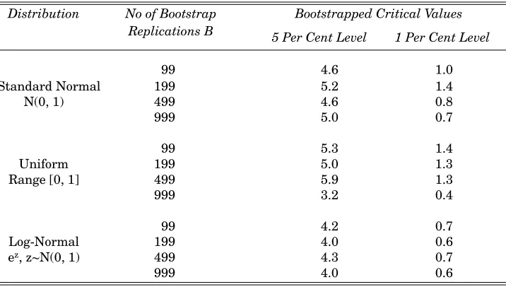
The Monte Carlo results set out in the tables illustrate the good small sample performance of bootstrapped critical values of R/S. Details of the data generation processes etc. used are given in the notes to the tables. Tables 1 and 2 refer to the i.i.d. distributions examined by Harrison and Treacy (1997). Table 1 sets out the empirical size of the R/S test statistic at the nominal 5 and 1 per cent levels using (i) bootstrapped critical values, (ii) the Beta approximation based critical values in Harrison and Treacy (1997, Table 10) and (iii) the asymptotic critical values in Lo (1991). The empirical size of the bootstrapped tests is good. Table 2 shows that a small number of bootstrap replications is sufficient to obtain reasonably accurate critical values.
Table 1: The Empirical Size of the R/S Statistic
Some Monte Carlo Results for the IID Normal, Uniform and Log-Normal Cases (1000 Replications, 99 Bootstrap Replications)
Bootstrapped Critical Harrison & Treacy’s Lo’s Asymptotic Distribution Sample Values Critical Values Critical Values
Size T
5 Per Cent 1 Per Cent 5 Per Cent 1 Per Cent 5 Per Cent 1 Per Cent
100 5.7 0.9 5.2 0.8 1.0 0.3
Standard 200 6.5 1.1 6.6 1.3 3.7 0.7
Normal 500 4.8 0.2 4.8 0.3 3.3 0.9
N(0, 1) 1000 4.6 1.1 4.3 1.0 4.3 1.0
100 3.2 0.4 3.5 0.5 1.5 0.1
Uniform 200 5.9 1.3 5.8 1.2 3.3 0.4
Range [0, 1] 500 5.5 1.1 5.9 1.1 3.9 0.5
1000 5.2 0.7 4.0 0.6 4.0 0.6
100 3.4 1.0 — — 1.2 0.1
Log-Normal 200 4.5 0.5 — — 1.4 0.2
ez, z~N(0, 1 ) 500 4.9 1.0 — — 2.3 0.4
1000 4.8 1.2 — — 3.3 0.4
Table 2: The Effect of Varying the Number of Bootstrap Replications on the Empirical Size of the R/S Statistic
Some Monte Carlo Results for the IID Normal, Uniform and Log-Normal Cases (1000 Replications, 100 Observations)
Distribution No of Bootstrap Bootstrapped Critical Values Replications B 5 Per Cent Level 1 Per Cent Level
99 4.6 1.0
Standard Normal 199 5.2 1.4
N(0, 1) 499 4.6 0.8
999 5.0 0.7
99 5.3 1.4
Uniform 199 5.0 1.3
Range [0, 1] 499 5.9 1.3
999 3.2 0.4
99 4.2 0.7
Log-Normal 199 4.0 0.6
ez, z~N(0, 1) 499 4.3 0.7
[image:5.499.68.426.402.605.2]T
able 3:
The Empirical Size of the Modified R
/S Statistic in the AR(1) Case
Some Monte Carlo Results Using the Post Blackened, Moving Block Bootstrap
(1000 Replications)
Sample
V
alue of AR(1)
Bootstrapped Critical Lo’ s Asymptotic DGP Size T Parameter ρ Critical V alues Critical V alues
5 Per Cent
1 Per Cent
5 Per Cent
1 Per Cent
Level Level Level Level 200 0.50 6.8 1.3 1.3 0.0 200 0.75 5.9 1.2 2.0 0.0 AR(1) 200 0.90 5.0 0.6 5.9 0.0 Standard 200 0.95 7.1 1.2 19.7 0.8 Normal Random 100 0.75 5.1 0.9 0.0 0.0 Errors 200 0.75 5.9 1.2 2.0 0.0 500 0.75 4.5 1.0 5.6 1.7 1000 0.75 4.8 1.1 12.2 2.8 200 0.50 4.5 0.6 0.5 0.0 200 0.75 5.0 1.0 1.4 0.0 AR(1) 200 0.90 5.2 0.6 5.4 0.1 Log 200 0.95 6.9 1.9 21.0 0.7 Normal Random 100 0.75 5.9 1.1 0.0 0.0 Errors 200 0.75 4.5 0.9 1.1 0.0 500 0.75 4.2 1.1 5.3 1.1 1000 0.75 5.5 1.1 10.2 2.9 Notes: The
AR(1) model is x
t = ρ xt–1 + u t
. The random error u
t
is either a standard normal or
, in the log normal case, the exponential of a
standard normal random variable. The post blackened, moving block bootstrap was used to calculate the bootstrapped critical val
ues. An
AR(10) model was used to pre-whiten the data.
A
block size of 10 was used for the moving block bootstrap. The Newey-W
est estima
tor was
Table 4: The Empirical Size of the Modified R/S Statistic in the MA(1) Case Some Monte Carlo Results using the Post Blackened, Moving Block Bootstrap
(1000 Replications, 200/500 Observations)
Sample Value of MA(1) Bootstrapped Critical Lo’s Asymptotic DGP Size T Parameter θ Values Critical Values
5 Per Cent 1 Per Cent 5 Per Cent 1 Per Cent
Level Level Level Level
0.50 4.8 1.5 1.2 0.0
MA(1) 200 0.75 4.2 0.7 0.2 0.0
Standard 0.90 4.7 0.6 0.7 0.3
Normal
Random 0.50 5.6 1.1 3.6 0.3
Errors 500 0.75 3.4 0.5 2.4 0.0
0.90 4.7 0.8 0.3 0.0
Notes: The MA(1) model is xt = ut + θut–1. See the Notes to Table 3 for details of the post blackened,
moving block bootstrap etc.
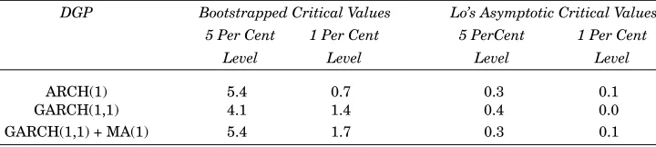
Table 5: The Empirical Size of the Modified R/S Statistic in the ARCH/ GARCH Case
Some Monte Carlo Results using the Post Blackened, Moving Block Bootstrap (1000 Replications, 100 Observations)
DGP Bootstrapped Critical Values Lo’s Asymptotic Critical Values 5 Per Cent 1 Per Cent 5 PerCent 1 Per Cent
Level Level Level Level
ARCH(1) 5.4 0.7 0.3 0.1
GARCH(1,1) 4.1 1.4 0.4 0.0
GARCH(1,1) + MA(1) 5.4 1.7 0.3 0.1
Notes: The GARCH(1,1) + MA(1) model is xt = et + 0.5et–1, et = htut, ht=1+0.3et2−1 + 0.4ht–1,
ut~N(0,1).The other two models are special cases. See the Notes to Table 3 for details of the post
blackened, moving block bootstrap etc.
[image:7.499.66.426.369.450.2]processes under the null. In summary, these results strongly suggest that the use of Lo’s asymptotic critical values for the R/S statistic be replaced or supplemented by the use of bootstrapped critical values obtained using the post blackened, moving block bootstrap.
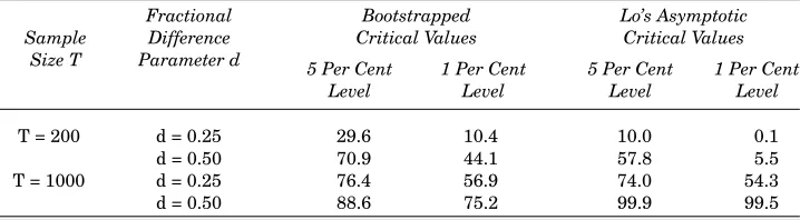
Table 6: The Empirical Power of the R/S Statistic in the Fractionally Integrated Case
Some Monte Carlo Results using the Post Blackened, Moving Block Bootstrap (1000 Replications, 200 Observations)
Fractional Bootstrapped Lo’s Asymptotic Sample Difference Critical Values Critical Values
Size T Parameter d 5 Per Cent 1 Per Cent 5 Per Cent 1 Per Cent
Level Level Level Level
T = 200 d = 0.25 29.6 10.4 10.0 0.1
d = 0.50 70.9 44.1 57.8 5.5
T = 1000 d = 0.25 76.4 56.9 74.0 54.3
d = 0.50 88.6 75.2 99.9 99.5
Notes: The model is xt= (1 - L)–dut with ut ~ N(0,1). The fractionally integrated series were generated
using the Choleski decomposition of the variance-covariance matrix. See the Notes to Table 3 for details of the post blackened, moving block bootstrap etc.
REFERENCES
ANIS, A.A., and E.H. LLOYD, 1976. “The Expected Value of the Adjusted Rescaled Hurst Range of Independent Normal Summands”, Biometrika, Vol. 63, pp. 111-116. CONNIFFE, D., and J.E. SPENCER, 1999. “Approximating the Distribution of the R/S
Statistic”, The Economic and Social Review, Vol. 31, No. 3, pp. 237-248.
BAILLIE, R.T., 1996. “Long Memory Processes and Fractional Differencing and Long Memory Processes”, Journal of Econometrics, Vol. 73, p. 5-59.
BERAN, J., 1994. Statistics for Long Memory Processes, London: Chapman and Hall. DAVIDSON, A.C., and D.V. HINKLEY, 1997. Bootstrap Methods and Their Application,
Cambridge: Cambridge University Press.
EFRON, B., and R.V. TIBSHIRAMI, 1993. An Introduction to the Bootstrap, London: Chapman and Hall/CRC.
HARRISON, M., and G. TREACY, 1997. “On the Small Sample Distribution of the R/S Statistic”, The Economic and Social Review, Vol. 28, No. 4, pp. 357-380.
HOROWITZ, J.L., 1994. “Bootstrap-Based Critical Values for the Information Matrix Test”, Journal of Econometrics, Vol. 61, pp. 395-411.
IZZELDIN, M., 1999. “Bootstrapping the Small Sample Distribution of the R/S Statistic”, MA Thesis, Dublin: University College, Dept. of Economics.
KWIATKOWSKI, D., P.C.B. PHILLIPS, P. SCHMIDT, and Y. SHIN, 1992. “Testing the Null Hypothesis of Stationarity Against the Alternative of a Unit Root: How Sure are we that Economic Time Series have a Unit Root?”, Journal of Econometrics, Vol. 73, pp. 159-178.
Fractionally Integrated Alternatives”, Journal of Econometrics, Vol. 73, pp. 285-302. LO, A.W., 1991. “Long Term Memory in Stock Market Prices”, Econometrica, Vol. 59, pp.
1279-1313.
MADDALA, G.S., and I.-M. KIM, 1999. Unit Roots, Cointegration and Structural Change, Cambridge: Cambridge University Press, pp. 328-333.
NEWEY, W.K., and K.D. WEST, 1987. “A Simple Positive Semi-Definite Heteroscedastic and Autocorrelation-Consistent Covariance Matrix”, Econometrica, Vol. 55, pp. 703-708.