Model Predictive Control for Deferrable Loads Scheduling
Thesis by Niangjun Chen
In Partial Fulfillment of the Requirements for the Degree of
Master of Science
California Institute of Technology Pasadena, California
2014
c
2014
Acknowledgements
I would like to express my gratitude towards my advisers Prof. Adam Wierman and Prof. Steven Low. I feel very fortunate and privileged receive enormous guidance and help from them. Their wisdom and encouragement help me overcome many obstacles during the past two years. I really learned a lot from both of them.
I am also grateful to my collaborators, Lachlan Andrew and Lingwen Gan. They have always provided insightful discussions and constructive suggestions. The atmosphere and environment of the RSRG, Computer Science department and Caltech are amazing and helpful. It is really a pleasure to work and study here.
Abstract
Real-time demand response is essential for handling the uncertainties of renewable genera-tion. Traditionally, demand response has been focused on large industrial and commercial loads, however it is expected that a large number of small residential loads such as air con-ditioners, dish washers, and electric vehicles will also participate in the coming years. The electricity consumption of these smaller loads, which we call deferrable loads, can be shifted over time, and thus be used (in aggregate) to compensate for the random fluctuations in renewable generation.
Contents
Acknowledgements iii
Abstract iv
1 Introduction 1
2 Real-time Deferrable Load Control 5
2.1 Model overview and Notation . . . 5
2.2 Renewable generation and non-deferrable load . . . 5
2.3 Deferrable load . . . 7
2.4 The deferrable load control problem . . . 9
3 Model Predictive Algorithm 11 3.1 Load control without uncertainty . . . 11
3.2 Load control with uncertainty . . . 13
4 Performance Analysis 18 4.1 Average-case Analysis . . . 18
4.1.1 The expected load variance of Algorithm 2 . . . 19
4.1.2 Improvement over static control . . . 21
4.2 Worst-case analysis . . . 23
4.3.1 Concentration bounds . . . 25
4.3.2 Bounds on the variance . . . 28
5 Simulation 30 5.1 Experimental setup . . . 30
5.2 Experimental results . . . 34
5.3 A case study . . . 38
6 Concluding Remarks 40 Bibliography 42 A Proofs of average case results 47 A.1 Proof of Theorem 1 . . . 47
A.2 Proof of Lemma 1 . . . 49
A.3 Proof of Lemma 2 . . . 50
A.4 Proof of Theorem 2 . . . 52
A.5 Proof of Corollary 3 . . . 53
A.6 Proof of Lemma 3 . . . 54
B Proofs of distributional results 56 B.1 Proof of Proposition 3 . . . 56
B.2 Proof of Theorem 3 . . . 61
Chapter 1
Introduction
The electricity grid is expected to change dramatically over the coming decades. Conven-tional coal and nuclear generation is being rapidly substituted by renewable generation such as wind and solar [9]. However, these renewables are difficult to predict. For example, wind generation prediction has a root-mean-square error of around 18% of the nameplate capac-ity looking 24 hours ahead [23]. Such high uncertainty in generation calls the traditional control strategy of “generation follows demand” into question.
Real-time demand response programs seek to induce dynamic demand management of customers’ electricity load in response to power supply conditions, e.g., by reducing or deferring power consumption in response to requests from the utility. Such programs have the potential to compensate for the uncertainties in renewables in real-time so as to ease the incorporation of renewable energy into the grid, and so are recognized as priority areas for the future smart grid by both the National Institute of Standards and Technology [37] and the Department of Energy [16].
high-lights the potential for scheduling deferrable loads in order to compensate for the random fluctuations of renewable energy.
However, realizing the potential of deferrable loads requires the coordination of a large number of distributed loads. Current approaches for achieving such coordination include 1) direct load control (DLC) by load serving entities (LSE) [27, 34, 19, 20], and 2) time-of-use pricing and other complex pricing structures [4, 11, 31]. DLC is the focus of this thesis since the LSE has full control over the loads. Specifically, this thesis focuses on decentralized DLC algorithms. The motivation for this approach is that, as the penetration of deferrable loads grows, the scale of the task of controlling deferrable loads will prevent centralized control and so distributed, decentralized coordination will become necessary.
Related work There is a growing body of work on decentralized direct load control algorithms. This literature focuses on both evaluating algorithms in simulation-based eval-uations [3, 36, 28] and on deriving theoretical performance guarantees [34, 19]. For example, [34] proposes a decentralized charging strategy for electric vehicles (EV) that is optimal if all EVs are identical, and [19] provides an algorithm for the setting when EVs are not necessarily identical.
Typically, the algorithms proposed in the literature, e.g., [3, 36, 28, 34, 19], have not considered uncertainties in renewable generation and deferrable load arrivals. However, of course, only predictions of these quantities are known ahead of time in practice, and the impact of prediction errors can be dramatic, e.g., see Figure 5.2.
perspective, this thesis first focuses on the “average-case” perspective, then we show via distributional analysis that the “average case” is indeed the representative case.
Summary of contributions We provide a model predictive algorithm for decentralized deferrable load control in the context of uncertain predictions about both future loads and future renewable generation. More specifically, in this thesis we propose a novel extension of the “optimal deferrable load control problem” studied in [19]. This extension incorpo-rates uncertainty about both deferrable and non-deferrable loads, in addition to inexact predictions of renewable generation; and then uses this problem to derive a new algorithm for deferrable load control. Further, we perform both analytic and trace-based perfor-mance analysis of the algorithm in order to quantify the impact of prediction uncertainties on deferrable load control. In particular, the contributions of the work are threefold.
First, we model renewable generation prediction as a Wiener filtering process [41] (Sec-tion 2.1), that is able to model any zero mean, sta(Sec-tionary predic(Sec-tion evolu(Sec-tions. Addi-tionally, the formulation includes a very general model for deferable loads that allows for heterogeneous deadlines and maximum charging rates, as well as stochastic arrivals.
Second, in the context of this model, we introduce a model predictive algorithm for deferrable load control with uncertainty (Section 3.2). The model predictive algorithm essentially solves a series of optimal control problems whose horizon lengths shrink with time. At any time, the algorithm uses only the information that is available, i.e., specifi-cations of deferrable loads that have already arrived and predictions on future loads and renewable generation. In this sense, the algorithm we propose is a (non-trivial) extension of the algorithm proposed in [19], which applies only in the case of exact knowledge of loads and renewables. A key technique introduced by the algorithm is the concept of a “pseudo deferrable load,” which is simulated at the utility to represent future deferrable load arrivals.
reduction in expected load variance achieved via deferrable load control, and (ii) the value of using model predictive control via our algorithm when compared with static (open-loop) control. The theorems in Section 4.1 characterize the impact of prediction inaccuracy on deferrable load control. These analytic results highlight that as the time horizon expands, the expected load variance obtained by our proposed algorithm approaches the optimal value (Corollary 3). Also, as the time horizon expands, the algorithm obtains an increas-ing variance reduction over the optimal static algorithm (Corollary 5, 6). Furthermore, in Section 5 we provide trace-based experiments using data from Southern California Edison and Alberta Electric System Operator to validate the analytic results. These experiments highlight that our proposed algorithm obtains a small suboptimality under high uncer-tainties of renewable generation, and has significant performance improvement over the optimal static control.
Chapter 2
Real-time Deferrable Load Control
2.1
Model overview and Notation
this thesis studies the design and analysis of real-time control algorithms for scheduling deferrable loads to compensate for the random fluctuations in renewable generation. In the following we present a model of this scenario that serves as the basis for our algorithm de-sign and performance evaluation. The model includes renewable generation, non-deferrable loads, and deferrable loads, which are described in turn. The key differentiation of this model from that of [19] is the inclusion of uncertainties (prediction errors) on future re-newable generation and loads.
Throughout, we consider a discrete-time model over a finite time horizon. The time horizon is divided into T time slots of equal length and labeled 1, . . . , T. In practice, the time horizon could be one day and the length of a time slot could be 10 minutes.
2.2
Renewable generation and non-deferrable load
Renewable generation like wind is stochastic and difficult to predict. Similarly, non-deferrable load including lights are hard to predict at a low aggregation level.
Since the focus is on scheduling deferrable loads, we aggregate renewable generation and non-deferrable load into one process termed the base load, b = {b(τ)}T
defined as the difference between non-deferrable load and renewable generation, and is a stochastic process.
To model the uncertainty of base load, we use a causal filter based model described as follows, and illustrated in Figure 2.1. In particular, the base load at timeτ is modeled as a random deviation δb = {δb(τ)}T
τ=1 around its expectation ¯b = {¯b(τ)}Tτ=1. The process ¯b is specified externally to the model, e.g., from historical data and weather report, and
the processδb(τ) is further modeled as an uncorrelated sequence of identically distributed random variables e ={e(τ)}T
τ=1 with mean 0 and variance σ2, passing through a causal filter. Specifically, let f = {f(τ)}∞τ=−∞ denote the impulse response of this causal filter and assume that f(0) = 1, thenf(τ) = 0 forτ <0 and
δb(τ) =
T
X
s=1
e(s)f(τ−s), τ = 1, . . . , T.
At timet= 1, . . . , T, a prediction algorithm can observe the sequencee(s) fors= 1, . . . , t, and predictsb as1
bt(τ) = ¯b(τ) + t
X
s=1
e(s)f(τ−s), τ = 1, . . . , T. (2.1)
Note thatbt(τ) =b(τ) for τ = 1, . . . , t sincef is causal.
Figure 2.1: Diagram of the notation and structure of the model for base load, i.e., non-deferrable load minus renewable generation.
This model allows for non-stationary base load through the specification of ¯b and a broad class of models for uncertainty viaf and e. In particular, two specific filters f that
1
we consider in detail later in the paper are:
1. A filter with finite but flat impulse response, i.e., there exists ∆>0 such that
f(t) =
1 if 0≤t <∆
0 otherwise;
2. A filter with an infinite and exponentially decaying impulse response, i.e., there exists a∈(0,1) such that
f(t) =
at ift≥0
0 otherwise.
These two filters provide simple but informative examples for our discussion in Section 4.1.
2.3
Deferrable load
To model deferrable loads we consider a setting whereN deferrable loads arrive over the time horizon, each requiring a certain amount of electricity by a given deadline. Further, a real-time algorithm has imperfect information about the arrival times and sizes of these deferrable loads.
More specifically, we assume a total ofN deferrable loads and label them in increasing order of their arrival times by 1, . . . , N, i.e., load n arrives no later than load n+ 1 for n= 1, . . . , N−1. Further, we defineN(t) as the number of loads that arrive before (or at) timetfort= 1, . . . , T and fix N(0) := 0. Thus, load 1, . . . , N(t) arrive before or at timet fort= 1, . . . , T and N(T) =N.
timet,pn(t), must be between given lower and upper boundspn(t) and pn(t), i.e.,
pn(t)≤pn(t)≤pn(t), n= 1, . . . , N, t= 1, . . . , T. (2.2)
These are specified externally to the model. For example, if an electric vehicle plugs in with Level II charging, then its power consumption must be within [0,3.3]kW. However, if it is not plugged in (has either not arrived yet or has already departed) then its power consumption is 0kW, i.e., within [0,0]kW. Further, we assume that a deferrable load n must withdraw a fixed amount of energyPn by its deadline, i.e.,
T
X
t=1
pn(t) =Pn, n= 1, . . . , N. (2.3)
Finally, theN deferrable loads arrive randomly throughout the time horizon. Define
a(t) :=
N(t)
X
n=N(t−1)+1
Pn (2.4)
as the total energy request of all deferrable loads that arrive at timetfort= 1, . . . , T. We assume that{a(t)}T
t=1is a sequence of independent identically distributed random variables with mean λand variances2. Further, define
A(t) :=
T
X
τ=t+1
a(τ) (2.5)
as the total energy requested after timetfort= 1, . . . , T.
In summary, at time t= 1, . . . , T, a real-time algorithm has full information about the deferrable loads that have arrived, i.e., pn,pn, andPn forn= 1, . . . , N(t), and knows the
2.4
The deferrable load control problem
We can now formally state the deferrable load control problem that is the focus of this thesis. Recall that the objective of real-time deferrable load control is to compensate for the random fluctuations in renewable generation and non-deferrable load in order to “flatten” theaggregate load d={d(t)}T
t=1, which is defined as
d(t) =b(t) +
N
X
n=1
pn(t), t= 1, . . . , T. (2.6)
In this thesis, we focus on minimizing the sample path variance of the aggregate load d, V(d), as a measure of “flatness”, that is defined as
V(d) = 1 T
T
X
t=1
d(t)− 1
T
T
X
τ=1 d(τ)
!2
. (2.7)
We can now formally specify the optimal deferrable load control (ODLC) problem that we seek to solve:
ODLC: min 1
T
T
X
t=1
d(t)− 1
T
T
X
τ=1 d(τ)
!2
(2.8)
over pn(t), d(t), ∀n, t
s.t. d(t) =b(t) +
N
X
n=1
pn(t), ∀t;
p
n(t)≤pn(t)≤pn(t), ∀n, t; T
X
t=1
pn(t) =Pn, ∀n.
the objective functionV(d) is replaced byf(d) =PT
Chapter 3
Model Predictive Algorithm
Given the optimal deferrable load control (ODLC) problem defined in (2.8), the first con-tribution of this thesis is to design an algorithm that solves ODLC in real-time, given uncertain predictions of base and deferrable loads.
There are two key challenges for the algorithm design. First, the algorithm has access only to uncertain predictions at any given time, i.e., at time t the algorithm only knows deferrable loads 1 toN(t) rather than 1 toN, and only knows the predictionbtinstead ofb
itself. Second, even if there was no uncertainty in predictions, solving the ODLC problem requires significant computational effort when there are a large number of deferrable loads. Motivated by these challenges, in this section we design a decentralized algorithm with strong performance guarantees even when there is uncertainty in the predictions. The algorithm builds on the work of [19], which provides a decentralized algorithm for the case without uncertainty in predictions. We present the details of the algorithm from [19] in Section 3.1 and then present a modification of the algorithm to handle uncertain predictions in Section 3.2.
3.1
Load control without uncertainty
the ODLC problem in (2.8) via a decentralized algorithm. Such a decentralized algorithm was proposed in [19], and we summarize the algorithm and its analysis here.
Algorithm definition: The algorithm from [19] is given in Algorithm 1. It is iterative and the superscripts in brackets denote the round of iteration. In each iteration k ≥ 0, there are two key steps: Step (ii) and (iii). In Step (ii), the utility calculates the average loadg(k)and broadcasts it to all deferrable loads. Note that the utility only needs to know the reported schedulep(nk), the base load b, and the number of deferrable loads N. It does
not need to know the constraints of the deferable loads. In Step (iii), each deferrable load nupdatesp(nk+1) by solving a convex optimization. The objective function has two terms.
The first term can be interpreted as the electricity bill if the electricity price was set to g(k). The second term vanishes as iterations continue.
Algorithm convergence results: Importantly, though Algorithm 1 is iterative, it converges very fast. In fact, the simulations in [19] stop the iterations after 15 rounds (i.e., K=15) in all cases because convergence is already achieved. Further, Algorithm 1 provably solves the ODLC problem given in (2.8) when there is no uncertainty, i.e., whenN(t) =N andbt=bfort= 1, . . . , T [19]. More precisely, letOdenote the set of optimal solutions to
(2.8), and defined(p,O) := minpˆ∈Okp−pˆkas the distance from a deferrable load schedule pto optimal deferrable load schedulesO.
Proposition 1 ([19]). When there is no uncertainty, i.e., N(t) = N and bt = b for
t= 1, . . . , T, the deferrable load schedulesp(k) obtained by Algorithm 1 converge to optimal schedules to ODLC, i.e.,d(p(k),O)→0 ask→ ∞.
A particular class of optimal solutions will be of interest to us later in the paper, so we define them here. Specifically, we call a feasible deferrable load schedulep = (p1, . . . , pN)
valley-filling, if there exists some constant C ∈R such that PNn=1pn(t) = (C−b(t))+ for
t= 1, . . . , T.
ODLC. Further, in such cases, all optimal schedules to ODLC have the same aggregate
load.
Note that valley-filling schedules tend to exist if there is a large number of deferrable loads, in such settings optimal solutions to ODLC are valley-filling.
3.2
Load control with uncertainty
Algorithm 1 provides a decentralized approach for solving the ODLC problem; however it assumes exact knowledge (certainty) about base load and deferrable loads. In this section, we adapt Algorithm 1 to the setting where there is uncertainty in base load and deferrable load predictions, while maintaining strong performance guarantees. In particular, in this section we assume that at time t, only the prediction bt is known, not b itself, and only
information about deferrable loads 1 toN(t) and the expectation of future energy requests
E(A(t)) are known.
Algorithm definition: To adapt Algorithm 1 to deal with uncertainty, the first step is straightforward. In particular, it is natural to replace the base load b by its prediction bt in Algorithm 1 to deal with the unavailability ofb.
However, dealing with unavailable future deferrable load information is trickier. To do this we use a pseudo deferrable load, which is simulated at the utility, to represent future deferrable loads. More specifically, letq ={q(τ)}T
τ=twithq(t) = 0 denote the power
consumption of the pseudo load, and assume that it requests E(A(t)) amount of energy, i.e.,
T
X
τ=t
q(τ) =E(A(t)). (3.1)
We also assume that q is point-wise upper and lower bounded by some upper and lower bounds q and q, i.e.,
Note thatq(t) =q(t) = 0. The bounds q and q should be set according to historical data. Here, for simplicity, we consider them to beq(τ) = 0 and q(τ) =∞ forτ =t+ 1, . . . , T.
Given the above setup, the utility solves the following problem at every time slot t= 1, . . . , T, to accommodate the availability of only partial information.
ODLC-t: min
T
X
τ=t
d(τ)− 1
T−t+ 1
T
X
s=t
d(s)
!2
(3.3)
over pn(τ), q(τ), d(τ), n≤N(t), τ ≥t
s.t. d(τ) =bt(τ) + N(t)
X
n=1
pn(τ) +q(τ), τ ≥t;
pn(τ)≤pn(τ)≤pn(τ), n≤N(t), τ ≥t; T
X
τ=t
pn(τ) =Pn(t), n≤N(t);
q(τ)≤q(τ)≤q(τ), τ ≥t;
T
X
τ=t
q(τ) =E(A(t))
where Pn(t) = Pn −Pτt−1=1pn(τ) is the energy to be consumed at or after time t, for
n= 1, . . . , N(t) and t= 1, . . . , T.
Now, adjusting Algorithm 1 to solve ODLC-t gives Algorithm 2, which is real-time and shrinking-horizon. Note that if base load prediction is exact (i.e., bt=b for t= 1, . . . , T)
and all deferrable loads arrive at the beginning of the time horizon (i.e., N(t) = N for t= 1, . . . , T), then ODLC-1 reduces to ODLC and Algorithm 2 reduces to Algorithm 1.
Algorithm convergence results: We provide analytic guarantees on the convergence and optimality of Algorithm 2. In particular, we prove that Algorithm 2 solves ODLC-t at every time slott. Specifically, let O(t) denote the set of optimal schedules to ODLC-t, and defined(p,O(t)) := min( ˆp,qˆ)∈O(t)kp−pˆkas the distance from a schedule p to optimal schedulesO(t) at timet, fort= 1, . . . , T.
2 converge to optimal schedules to ODLC-t, i.e., d(p(k),O(t))→0 ask→ ∞.
The theorem is proved in Appendix A.1. Though iterative, Algorithm 2 converges fast, similar to Algorithm 1. In the simulations, settingK = 15 is enough for all test cases.
Similar to Proposition 2, “t-valley-filling” provides a simple characterization of the solutions to ODLC-t. Specifically, at time t= 1, . . . , T, a feasible schedule (p, q) is called t-valley-filling, if there exists some constantC(t)∈Rsuch that
q(τ) +
N(t)
X
n=1
pn(τ) = (C(t)−bt(τ))+, τ =t, . . . , T. (3.4)
Given this definition of t-valley-filling, the following corollary follows immediately from Proposition 2.
Corollary 1. At time t = 1, . . . , T, a t-valley-filling deferrable load schedule, if exists, solves ODLC-t. Furthermore, in such cases, all optimal schedules to ODLC-t have the
same aggregate load.
Algorithm 1 Deferrable load control without uncertainty
Input: The utility knows the base load b and the number N of deferrable loads. Each loadn∈ {1, . . . , N}knows its energy requestPnand power consumption boundspnand
pn. The utility setsK, the number of iterations.
Output: Deferrable load schedulep= (p1, . . . , pN).
(i) Set k←0 and intitialize the schedulep(k) as p(nk)(t)←0, t= 1, . . . , T, n= 1, . . . , N.
(ii) The utility calculates the average loadg(k)=d(k)/N,
g(k)(t)← 1
N b(t) +
N
X
n=1 p(nk)(t)
!
, t= 1, . . . , T,
and broadcasts g(k) to all deferrable loads.
(iii) Each load nupdates a new schedule p(nk+1) by solving
min
T
X
τ=1
g(k)(τ)pn(τ) +
1 2
pn(τ)−p(nk)(τ)
2
over pn(1), . . . , pn(T)
s.t. pn(τ)≤pn(τ)≤pn(τ), ∀τ; T
X
τ=1
pn(τ) =Pn,
and reports p(nk+1) to the utility.
Algorithm 2 Deferrable load control with uncertainty
Input: At time t, the utility knows the prediction bt of base load and the number N(t)
of deferrable loads. Each deferrable load n ∈ {1, . . . , N(t)} knows its future energy requestPn(t) and power consumption boundspnandpn. The utility setsK, the number
iterations.
Output: At time t, output the power consumptionpn(t) for deferrable loads 1, . . . , N(t).
At time slot t= 1, . . . , T:
(i) Setk←0. Each deferrable loadn∈ {1, . . . , N(t)}initializes its schedule{p(0)n (τ)}Tτ=t
as
p(0)n (τ)←
(
p(nK)(τ) ifn≤N(t−1)
0 ifn > N(t−1), τ =t, . . . , T
wherep(nK) is the schedule of load nin iterationK of the previous time slott−1.
(ii) The utility solves
min
T
X
τ=t
bt(τ) + N(t)
X
n=1
p(nk)(τ) +q(τ)
2
over q(t), . . . , q(T)
s.t. q(τ)≤q(τ)≤q(τ), τ ≥t;
T
X
τ=t
q(τ) =E(A(t))
to obtain a pseudo schedule {q(k)(τ)}T
τ=t. The utility then calculates the average
aggregate load per deferrable loadg(k) as
g(k)(τ)← 1
N(t)
bt(τ) + N(t)
X
n=1
p(nk)(τ) +q(k)(τ)
forτ =t, . . . , T, and broadcasts {g(k)(τ)}T
τ=tto deferrable loads n= 1, . . . , N(t).
(iii) Each deferrable load n= 1, . . . , N(t) solves
min
T
X
τ=t
g(k)(τ)pn(τ) +
1 2
pn(τ)−p(nk)(τ)
2
over pn(t), . . . , pn(T)
s.t. pn(τ)≤pn(τ)≤pn(τ), τ ≥t; T
X
τ=t
pn(τ) =Pn(t),
to obtain a new schedule{p(nk+1)(τ)}Tτ=t, and reports {pkn+1(τ)}Tτ=t to the utility.
(iv) Setk←k+ 1. If k < K, go to Step (ii).
Chapter 4
Performance Analysis
4.1
Average-case Analysis
To this point, we have shown that Algorithm 2 makes “optimal” decisions with the in-formation available at every time slot, i.e., it solves ODLC-t at time t for t = 1, . . . , T. However, these decisions are still suboptimal compared to what could be achieved if ex-act information was available. In this section, our goal is to understand the impex-act of uncertainty on the performance. In particular, we study two questions:
(i) How do the uncertainties about base load and deferrable loads impact the expected sample path load variance obtained by Algorithm 2?
(ii) What is the improvement of using the real-time control provided by Algorithm 2 over using the optimal static control?
under which (3.4) implies
d(t) =C(t) = 1 T−t+ 1
T
X
τ=t
bt(τ) +E(A(t)) +
N(t)
X
n=1 Pn(t)
(4.1)
fort= 1, . . . , T. Thus, equation (4.1) defines the model we use for the performance analysis of Algorithm 2.
4.1.1 The expected load variance of Algorithm 2
We start by calculating the expected load variance, E(V), of Algorithm 2. The goal is to understand how uncertainty about base load and deferrable loads impacts the load variance. Note that, if there are no base load prediction errors and deferrable loads arrive at the beginning of the time horizon, then Algorithm 2 obtains optimal schedules that have zero load variance. In contrast, when there are base load prediction errors and stochastic deferrable load arrivals, the expected load variance is given by the following theorem.
To state the result, recall that {f(t)}∞t=−∞is the causal filter modeling the correlation of base load and defineF(t) :=Pt
s=0f(s) for t= 0, . . . , T.
Theorem 2. The expected load varianceE(V) obtained by Algorithm 2 is
E(V) = s 2 T
T
X
t=2 1 t +
σ2 T2
T−1
X
t=0
F2(t)T−t−1
t+ 1 . (4.2)
The theorem is proved in Appendix A.4.
Theorem 2 explicitly states the interaction of the variability of base load prediction (σ) and deferrable load prediction (s) with the horizon length T. Besides, it highlights the correlation of base load prediction error through F. More specifically, the expected load varianceE(V) tends to 0 as the uncertainties in base load and deferrable loads vanish, i.e., σ→0 and s→0.
Another remark about Theorem 2 is that the two terms in (4.2) correspond to the impact of the uncertainties in deferrable loads and base load respectively. In particular, Theorem 2 is proved in Section A.4 by analyzing these two cases separately and then combining the results. Specifically, the following two lemmas are the key pieces in the proof of Theorem 2, but are also of interest in their own right.
Lemma 1. If there is no base load prediction error, i.e., bt=b for t= 1, . . . , T, then the
expected load variance obtained by Algorithm 2 is
E(V) =s2
PT
t=2 1
t
T ≈s 2lnT
T .
The lemma is proved in Appendix A.2.
Lemma 2. If there are no deferrable load arrivals after time 1, i.e., N(t) = N for t = 1, . . . , T, then the expected load variance obtained by Algorithm 2 is
E(V) = σ 2 T2
T−1
X
t=0
F2(t)T −t−1 t+ 1 .
The lemma is proved in Appendix A.3.
Lemma 1 highlights that the more uncertainty in deferrable load arrival, i.e., the larger s, the larger the expected load variance E(V). On the other hand, the longer the time horizonT, the smaller the expected load varianceE(V).
Similarly, Lemma 2 highlights that a larger base load prediction error, i.e., a larger σ, results in a larger expected load variance E(V). However, if the impulse response
{f(t)}∞t=−∞ of the modeling filter of the base load decays fast enough with t, then the following corollary highlights that the expected load variance actually tends to 0 as time horizonT increases despite the uncertainty of base load predictions.
obtained by Algorithm 2 satisfiesE(V)→0 as T → ∞.
The corollary is proved in Appendix A.5.
4.1.2 Improvement over static control
The goal of this section is to quantify the improvement of real-time control via Algorithm 2 over the optimal static (open-loop) control. To be more specific, we compare the expected load varianceE(V) obtained by the real-time control Algorithm 2, with the expected load varianceE(V0) obtained by the optimal static control, which only uses base load prediction at the beginning of the time horizon (i.e., ¯b) to compute deferrable load schedules. We assumeN(t) =N fort= 1, . . . , T in this section since otherwise any static control cannot obtain a schedule for all deferrable loads. Thus, the interpretation of the results that follow is as a quantification of the value of incorporating updated base load predictions into the deferrable load controller.
To begin the analysis, note that E(V) for this setting is given in Lemma 2. Further, it can be verified that the optimal static control is to solve ODLC withb replaced by ¯b, and the corresponding expected load varianceE(V0) is given by the following lemma.
Lemma 3. If there is no stochastic load arrival, i.e., N(t) =N for t= 1, . . . , T, then the expected load variance E(V0) obtained by the optimal static control is
E(V0) = σ 2 T2
T−1
X
t=0
T(T −t)f2(t)−F2(t)
.
The lemma is proved in Appendix A.6.
Next, comparing E(V) and E(V0) given in Lemma 2 and 3 shows that Algorithm 2 al-ways obtains a smaller expected load variance than the optimal static control. Specifically,
1, . . . , T, then
E(V0)−E(V) = σ 2 T
T
X
t=1 1 2t
t−1
X
m=0
t−1
X
n=0
(f(m)−f(n))2 ≥0.
The corollary is proved in the extended version [22].
Corollary 4 highlights that Algorithm 2 is guaranteed to obtain a smaller expected load variance than the optimal static control. The next step is to quantify how much smaller
E(V) is in comparison withE(V0).
To do this we compute the ratio E(V0)/E(V). Unfortunately, the general expression for the ratio is too complex to provide insight, so we consider two representative cases for the impulse response f(t) of the causal filter in order to obtain insights. Specifically, we consider examples (i) and (ii) from Section 2.2. Briefly, in (i) f(t) is finite and in (ii) f(t) is infinite but decays exponentially int. For these two cases, the ratio E(V0)/E(V) is summarized in the following corollaries.
Corollary 5. If there is no deferrable load arrival after time 1, i.e., N(t) = N for t = 1, . . . , T, and there exists ∆>0 such that
f(t) =
1 if 0≤t <∆
0 otherwise,
then
E(V0) E(V) =
T /∆ ln(T /∆)
1 +O
1 ln(T /∆)
.
The corollary is proved in the extended version [22].
1, . . . , T, and there exists a∈(0,1)such that
f(t) =
at if t≥0
0 otherwise,
then
E(V0) E(V) =
1−a 1 +a
T lnT
1 +O
ln lnT lnT
.
The corollary is proved in the extended version [22].
Corollary 5 highlights that, in the case where f is finite, if we define λ=T /∆ as the ratio of time horizon to filter length, then the load reduction roughly scales as λ/ln(λ). Thus, the longer the time horizon is in comparison to the filter length, the larger expected load variance reduction we obtain from using Algorithm 2 as compared with the optimal static control.
Similarly, Corollary 6 highlights that, in the case where f is infinite and exponentially decaying, the expected load variance reduction scales with T as T /lnT with coefficient (1−a)/(1 +a). Thus, the smallera is, which means the faster f dies out, the more load variance reduction we obtain by using real-time control. This is similar to having a smaller ∆ in the previous case.
4.2
Worst-case analysis
The results surveyed above highlight that Algorithm 2 performs well on average; however, it is often important to guarantee more than good average case performance. For that reason, many results in the literature focus on worst case analysis, e.g., [30, 33, 6]. While no existing results apply directly to the setting of this thesis, it is straightforward to see that the worst-case performance of Algorithm 2 is quite bad.
Definition 1. We say thatprediction errors are bounded if there exist 1 and 2 such that, at any timet= 1, . . . , T,
|a(t)−λ| ≤1, |e(t)| ≤2. (4.3)
In this situation, it is straightforward to see that the worst case performance of Al-gorithm 2 can potentially be quite bad. For two real numbers a, b ∈ R, define a∨b := max{a, b}.
Proposition 3. If at-valley-filling solution exists fort= 1,2, . . . , T, and prediction errors are bounded by 1 and 2 as in (4.3), then the worst-case load variance supa,eV achieved
by Algorithm 2 is
sup
a,e
V = 21 1− 1
T
T
X
k=1 1 k
!
+ 2 2 T2
T−1
X
τ=0
T−1
X
s=0
T
τ ∨s+ 1−1
|F(τ)F(s)|.
The worst-case performance is achieved when all prediction errors on the load arrivals are equal to 1 while all prediction errors on the generation are equal to 2 in magnitude with the appropriate signs—the case where a(t) =λ+1 and e(t) =2·sgn(F(T−t)) for allt.
Corollary 7. If a t-valley-filling solution exists for t = 1,2, . . . , T, and prediction errors are bounded by 1 and 2 as in (4.3), then the worst-case load variance supa,eV achieved by Algorithm 2 is lower bounded as
sup
a,e
V ≥ 21 1− 1
T
T
X
k=1 1 k
!
≈ 21
1− lnT
T
Interestingly, the form of Corollary 7 implies that, in the worst-case, Algorithm 2 can be as bad as having no control at all: the time averaged load variance behaves like the worst one step load variance. Meanwhile, recall from Proposition ?? that the average performanceE(V)→0 asT → ∞. Hence, while the the load varianceV has a small mean
E(V), it can be quite large in the worst case.
4.3
Distributional analysis
The contrast between the worst-case analysis (Proposition 3) and average-case analysis (Proposition??) motivates the main goal of this thesis – to understand how often the “bad cases,” whereV takes large values, happen. That is, we want to understand what typical variations ofV under Algorithm 2 look like.
4.3.1 Concentration bounds
We start with analyzing the tail probability ofV. Concretely, our focus is on
Vη := min{c∈R|V ≤cwith probability η},
which denotes the minimum valuecsuch that V ≤cwith probability η forη∈[0,1]. Our main result provides upper bounds onVη, for large values of η, for arbitrary of prediction
error distributions.
More specifically, we prove that with high probability, the load variance of Algorithm 2 does not deviate much from its average-case performance, i.e., we prove a concentration result for model predictive deferable load control.
obtained by Algorithm 2 satisfies a Bernstein type concentration, i.e.,
P(V −EV > t)≤exp
−t2 162λ
1(2EV +t)
(4.4)
where = max(1, 2) and
λ1 = lnT
T + 1 T2
T−1
X
t=0
F2(t)T−t+ 1 t+ 1 .
The theorem is proven in Appendix B.2.
To build intuition, the tail probability bound of V in (4.4) can be simplified for two different regimes oft as
P(V −EV > t)≤
exp48−2λt2 1EV
, t <EV
exp48−2tλ 1
, t≥EV.
(4.5)
Though looser than that in (4.4), the tail bound in (4.5) highlights thatV has a Gaussian tail probability bound when t < EV and an Exponential tail probability bound when t≥EV.
Theorem 3 relates the tail behavior ofV with the maximum prediction errorand the error correlationF over time. It implies that the actual performance of Algorithm 2 does not deviate much from its mean. To illustrate this, consider the following example where the prediction on baseload is precise, since the parameter λ1 has a simple expression in this scenario.
Example 1. Suppose that the baseload prediction is precise, i.e.,2= 0. Then the average load variance is
E[V] = s 2 T
T
X
t=2 1 t ≈s
and the tail bound in Theorem 3 can be simplified as
P(V −EV > cEV)≤exp
− c
2 2 +c
s2 162
.
Recall that constant s is the variance of a and constant is the maximum deviation of a from its mean. The above expression shows that, with high probability, V is at most a constant c+ 1times of its mean EV.
More generally, the quantity λ1 controls the decaying speed of the tail bound in (4.4): the smallerλ1, the faster the tail boundP(V−EV > t) decays int, and the load varianceV achieved by Algorithm 2 concentrates sharper around its meanEV. The following corollary highlights thatλ1 tends to 0 asT increases, provided that the error correlationf(t) decays fast enough int. Note that the condition on f is the same for Corollary 8 and Proposition
??.
Corollary 8. Under the assumptions of Theorem 3, if the error correlationf ∼O(t−12−α)
for some α >0, then λ1 →0 asT → ∞.
A detailed proof of Theorem 3 is included in the Appendix; however it is useful to provide some informal intuition for the argument used.
In general, tail probability bounds can be obtained by controlling the moments of a random variable. For example, the Markov inequality gives inverse linear tail probability bound using the first moment, and the Chebyshev inequality provides inverse quadratic tail probability bound using the second moment. However, the bound we obtained in Theorem 3 approaches 0 much faster for large t than the aforementioned Markov and Chebyshev bounds. This is done by controlling the moment generating function ofV using the convex Log-Sobolev inequality.
one of the sources a(t) or e(t) of the randomness changes. Instead, we exploit the fact that the gradient ofV is bounded by a linear function of itself (similar but slightly differ-ent from the “self-bounding” property defined in [7]). Using this property together with Log-Sobolev inequality in the product measure gives us a nice way to bound the entropy of V. After this we apply the Herbst’s argument [29] to compute a good estimate on the concentration of V.
4.3.2 Bounds on the variance
To further understand the scale of typical load varianceV under Algorithm 2, it is useful to also study the variance. In addition, the form of the variance highlights the impact of the tight concentration shown in Theorem 3.
Theorem 4. Suppose a t-valley-filling solution exists for t = 1,2, . . . , T, and prediction errors are bounded by 1 and 2 as in (4.3). Then the variance var(V) of V obtained by Algorithm 2 is bounded above by
var(V)≤
41slnT T
2
+ 42σ
T2
T−1
X
t=0
F2(t)T−t+ 1 t+ 1
!2
. (4.6)
To interpret this result, let var(V) denote the upper bound on var(V) provided in (4.6). Theorem 4 implies that EV and
q
var(V) scale similarly with T. In particular, the first term sT2 PT
t=2 1t in EV scales with T as Ω(lnT /T) while the first term (41slnT /T)
2 in var(V) scales with T as Ω (lnT /T)2
, and the second terms in EV and var(V) have the same relationship. Hence, the standard deviation pvar(V), which is upper bounded by
q
Corollary 9. Under the assumptions in Theorem 4, fort >0,
P(|V −EV|> t)
≤ 1
t2
41slnT T
2
+ 42σ T2
T−1
X
τ=0
F2(τ)T −τ + 1 τ + 1
!2
. (4.7)
While the tail bound (4.4) in Theorem 3 scales at least exponentially int, the Chebyshev inequality only provides a tail bound (4.7) that scales inverse quadratically int. Hence for large t, (4.4) provides a much tighter tail bound. However for small values of t, the tail bound (4.7) is usually tighter since the variance var(V) is well estimated in (4.6).
Furthermore, the variance var(V) vanishes as T expands, provided that f(t) decays sufficiently fast ast grows, as formally stated in the following corollary.
Corollary 10. Under the assumptions of Theorem 4, if the error correlationf ∼O(t−12−α)
for some α >0, then var(V)→0 as T → ∞.
Chapter 5
Simulation
In this Chapter we use trace-based experiments to explore the generality of the analytic results in the previous section. In particular, the results in the previous section characterize the expected load variance obtained by Algorithm 2 as a function of prediction uncertain-ties, and quantify the improvement of Algorithm 2 over the optimal static (open-loop) controller. However, the analytic results make simplifying assumptions on the form of un-certainties and solution schedules (equation (4.1)). Therefore, it is important to assess the performance of the algorithm using real-world data.
5.1
Experimental setup
The numerical experiments we perform use a time horizon of 24 hours, from 20:00 to 20:00 on the following day. The time slot length is 10 minutes, which is the granularity of the data we have obtained about renewable generation.
20:00 4:00 12:00 20:00 0.4
0.5 0.6 0.7 0.8 0.9 1 1.1
time of day
non−deferrable load (kW/household)
(a) non-deferrable load
20:000 4:00 12:00 20:00
0.1 0.2 0.3 0.4
time of day
renewable generation (kW/household)
Jan. 1st~2nd, 2006 Apr. 1st~2nd, 2007 Jul. 1st~2nd, 2008 Oct. 1st~2nd, 2009
(b) wind generation
0h 8h 16h 24h
0 20 40 60 80 100
time looking ahead
normalized wind prediction error (%)
[image:37.612.114.499.80.225.2](c) prediction error over time
Figure 5.1: Illustration of the traces used in the experiments. (a) shows the average residential load in the service area of Southern California Edison in 2012. (b) shows the total wind power generation of the Alberta Electric System Operator scaled to represent 20% penetration. (c) shows the normalized root-mean-square wind prediction error as a function of the time looking ahead for the model used in the experiments.
over the time horizon of a day is taken to be the average over the 366 days in 2012 as in Figure 5.1a, and assumed to be known to the utility at the beginning of the time horizon. In practice, non-deferrable load at the substation feeder level can be predicted within 1–3% root-mean-square error looking 24 hours ahead [18].
The renewable generation traces we use come from the 10-minute historical data for total wind power generation of the Alberta Electric System Operator from 2004 to 2009 [5]. In the simulations, we scale the wind power generation so that its average over the 6 years corresponds to a number of penetration levels in the range between 5% and 30%, and pick the wind power generation of a randomly chosen day as the renewable generation during each run. Figure 5.1b shows the wind power generation for four representative days, one for each season, after scaling to 20% penetration.
We assume that the renewable generation is not precisely known until it is realized, but that a prediction of the generation, which improves over time, is available to the utility. The modeling of prediction evolution over time is according to a martingale forecasting process [25, 24], which is a standard model for an unbiased prediction process that improves over time.
the prediction error wt(τ)−w(τ) at time t < τ is the sum of a sequence of independent
random variables ns(τ) as
wt(τ) =w(τ) + τ
X
s=t+1
ns(τ), 0≤t < τ ≤T.
Here w0(τ) is the wind prediction without any observation, i.e., the expected wind gener-ation ¯w(τ) at the beginning of the time horizon (used by static control).
The random variables ns(τ) are assumed to be Gaussian with mean 0. Their variances
are chosen as
E(n2s(τ)) =
σ2
τ−s+ 1, 1≤s≤τ ≤T
whereσ >0 is such that the root-mean-square prediction errorpE(w0(T)−w(T))2 look-ing T time slots (i.e., 24 hours) ahead is 0%–22.5% of the nameplate wind generation capacity.1 According to this choice of the variances ofns(τ), root-mean-square prediction
error only depends on how far ahead the prediction is, in particular as in Figure 5.1c. This choice is motivated by [23].
Deferrable loads For simplicity, we consider the hypothetical case where all deferrable loads are electric vehicles. Since historical data for electric vehicle usage is not available, we are forced to use synthetic traces for this component of the experiments. Specifically, in the simulations the electric vehicles are considered to be identical, each requests 10kWh electricity by a deadline 8 hours after it arrives, and each must consume power at a rate within [0,3.3]kW after it arrives and before its deadline.
In the simulations, the arrival process starts at 20:00 and ends at 12:00 the next day so that the deadlines of all electric vehicles lie within the time horizon of 24 hours. In each time slot during the arrival process, we assume that the number of arriving electric vehicles is uniformly distributed in [0.8λ,1.2λ], whereλ is chosen so that electric vehicles
1
(on average) account for 5%–30% of the non-deferrable loads. While this synthetic workload is simplistic, the results we report are representative of more complex setups as well.
Uncertainty about deferrable load arrivals is captured as follows. The prediction
E(A(t)) of future deferrable load total energy request is simply the arrival rate λ times the length of the rest of the arrival processT0−twhereT0 is the end of the arrival process (12:00), i.e.,
E(A(t)) =λ(T0−t), t= 1, . . . , T0.
Ift > T0, i.e., the deferrable load arrival process has ended, thenE(A(t)) = 0.
Baselines for comparison Our goal in the simulations is to contrast the performance of Algorithm 2 with a number of common benchmarks to tease apart the impact of real-time control and the impact of different forms of uncertainty. To this end, we consider four controllers in our experiments:
(i) Offline optimal control: The controller has full knowledge about the base load and deferrable loads, and solves the ODLC problem offline. It is not realistic in practice, but serves as a benchmark for the other controllers since offline optimal control obtains the smallest possible load variance.
(ii) Static control with exact deferrable load arrival information: The controller has full knowledge about deferrable loads (including those that have not arrived), but uses only the prediction of base load that is available at the beginning of the time horizon to compute a deferrable load schedule that minimizes the expected load variance. This static control is still unrealistic since a deferrable load is known only after it arrives. But, this controller corresponds to what is considered in prior works, e.g., [34, 19, 20].
uses the prediction of base load that is available at the current time slot to update the deferrable load schedule by minimizing the expected load variance to go, i.e., Algo-rithm 2 withN(t) =N fort= 1, . . . , T. The control is unrealistic since a deferrable load is known only after it arrives; however it provides the natural comparison for case (ii) above.
(iv) Real-time control without exact deferrable load arrival information, i.e., Algorithm 2. This corresponds to the realistic scenario where only predictions are available about future deferrable loads and base load. The comparison with case (iii) highlights the impact of deferrable load arrival uncertainties.
The performance measure that we show in all plots is the “suboptimality” of the con-trollers, which we define as
η:= V −V opt Vopt ,
where V is the load variance obtained by the controller and Vopt is the load variance obtained by the offline optimal, i.e., case (i) above. Thus, the lines in the figures correspond to cases (ii)-(iv).
5.2
Experimental results
Our experimental results focus on two main goals: (i) understanding the impact of predic-tion accuracy on the expected load variance obtained by deferrable load control algorithms, and (ii) contrasting the real-time (closed-loop) control of Algorithm 2 with the optimal static (open-loop) controller. We focus on the impact of three key factors: wind prediction error, the penetration of deferrable load, and the penetration of renewable energy.
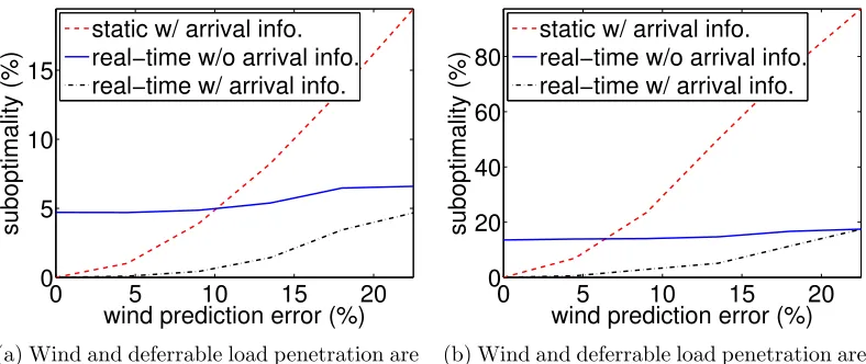
root-mean-square wind prediction errors (0%–22.5% of the nameplate capacity looking 24 hours ahead). The results are summarized in Figure 5.2a. It is not surprising that suboptimality of both the static and the real-time controllers that have exact information about deferrable load arrivals is zero when the wind prediction error is 0, since there is no uncertainty for these controllers in this case.
0 5 10 15 20
0 5 10 15
wind prediction error (%)
suboptimality (%)
static w/ arrival info. real−time w/o arrival info. real−time w/ arrival info.
(a) Wind and deferrable load penetration are both 10%.
0 5 10 15 20
0 20 40 60 80
wind prediction error (%)
suboptimality (%)
static w/ arrival info. real−time w/o arrival info. real−time w/ arrival info.
[image:41.612.110.504.198.364.2](b) Wind and deferrable load penetration are both 20%.
Figure 5.2: Illustration of the impact of wind prediction error on suboptimality of load variance.
As prediction error increases, the suboptimality of both the static and the real-time con-trol increases. However, notably, the suboptimality of real-time concon-trol grows much more slowly than that of static control, and remains small (¡4.7%) if deferrable load arrivals are known, over the whole range 0%–22.5% of wind prediction error. At 22.5% prediction error, the suboptimality of static control is 4.2 times that of real-time control. This highlights that real-time control mitigates the influence of imprecise base load prediction over time.
loads and the adaptive control does not.
As prediction error increases, the suboptimality of the real-time control with or with-out deferrable load arrival information gets close, i.e., the benefit of knowing additional information on future deferrable load arrivals vanishes as base load uncertainty increases. This is because the additional information is used to overfit the base load prediction error. The same comparison is shown in Figure 5.2b for the case where renewable and de-ferrable load penetration are both 20%. Qualitatively the conclusions are the same, however at this higher penetration the contrast between the resilience of adaptive control and static control is magnified, while the benefit of knowing deferrable load arrival information is minified. In particular, real-time control without arrival information beats static control with arrival information, at a lower (around 7%) wind prediction error, and knowing de-ferrable load arrival information does not reduce suboptimality of real-time control with 22.5% wind prediction error.
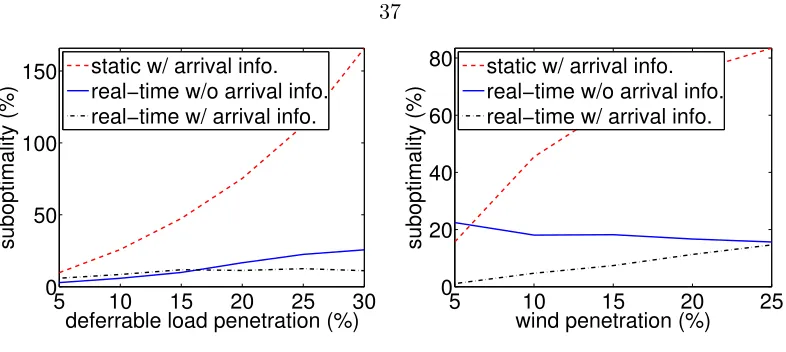
The impact of deferrable load penetration Next, we look at the impact of deferrable load penetration on the performance of the various controllers. To do this, we fix the wind penetration level to be 20% and wind prediction error looking 24 hours ahead to be 18%, and simulate the load variance obtained under different deferrable load penetration levels (5%–30%). The results are summarized in Figure 5.3a.
Not surprisingly, if future deferrable loads are known and uncertainty only comes from base load prediction error, then the suboptimality of real-time control is very small (¡11.2%) over the whole range 5%–30% of deferrable load penetration, while the suboptimality of static control increases with deferrable load penetration, up to as high as 166% (14.9 times that of real-time control) at 30% deferrable load penetration.
5 10 15 20 25 30 0
50 100 150
deferrable load penetration (%)
suboptimality (%)
static w/ arrival info. real−time w/o arrival info. real−time w/ arrival info.
(a) Impact of deferrable load penetration
5 10 15 20 25
0 20 40 60 80
wind penetration (%)
suboptimality (%)
static w/ arrival info. real−time w/o arrival info. real−time w/ arrival info.
[image:43.612.111.504.75.251.2](b) Impact of wind penetration
Figure 5.3: Suboptimality of load variance as a function of (a) deferrable load penetration and (b) wind penetration. In (a) the wind penetration is 20% and in (b) the deferrable load penetration is 20%. In both, the wind prediction error looking 24 hours ahead is 18%.
deferrable load penetration. The highest suboptimality 25.7% occurs at 30% deferrable load penetration, and is less than 1/6 of the suboptimality of static control, which assumes exact deferrable load arrival information.
The impact of renewable penetration Finally, we study the impact of renewable penetration. To do this we fix the deferrable load penetration level to be 20% and the wind prediction error looking 24 hours ahead to be 18%, and simulate the load variance obtained by the 4 test cases under different wind penetration levels (5%–25%). The results are summarized in Figure 5.3b.
deferrable loads, the suboptimality of real-time control becomes bigger. However, it still eventually outperforms the optimal static controller at around 6% wind penetration, despite the fact that the optimal static controller is using exact information about deferrable loads.
5.3
A case study
Theorems 3 and 4 provide theoretical guarantees that the load variance V obtained by Algorithm 2 concentrates around its mean, if prediction errors are bounded as in (4.3) and error correlation decays sufficiently fast (c.f. Corollary 2). Thus, they give the intuition that the expected performance of Algorithm 2 is a useful metric to focus on, and does indeed give an indication of the “typical” performance of the algorithm.
However, our analysis is based on the assumption that at-valley-filling solution exists, which relies on the penetration of deferrable load being high enough. This is a neces-sary technical assumption for our analysis, and has been used by the previous analysis of Algorithm 2 as well, e.g., [21].
Given this assumption in the analytic results, it is important to understand the ro-bustness of the results to this assumption. To that end, here we provide a case study to demonstrate that this intuition is robust to thet-valley-filling assumption.
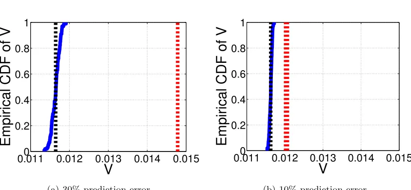
In our case study, we mimic the setting of [21], where an average-case analysis of Algorithm 2 is performed. In particular, we use 24 hour residential load trace in the Southern California Edison (SCE) service area averaged over the year 2012 and 2013 [2] as the non-deferrable load, and wind power generation data from the Alberta Electric System Operator from 2004 to 2012 [1]. The wind power generation data is scaled so that its average over 9 years corresponds to 30% penetration level, and pick the wind generation of a random day as renewable during each run. We generate random prediction error in baseload and arrival of deferrable load similar to [21].
0.0110 0.012 0.013 0.014 0.015 0.2
0.4 0.6 0.8 1
V
Empirical CDF of V
(a) 30% prediction error
0.0110 0.012 0.013 0.014 0.015
0.2 0.4 0.6 0.8 1
V
Empirical CDF of V
[image:45.612.98.519.85.280.2](b) 10% prediction error
Figure 5.4: The empirical cumulative distribution function of the load variance under Algorithm 2 over 24 hour control horizon using real data. The red line represents the analytic bound on the 90% confidence interval computed from Theorem 3, and the black line shows the empirical mean.
Chapter 6
Concluding Remarks
The main limitation in our analysis (which is also true for the prior stochastic analysis of model predictive deferrable load control) is the assumption that at-valley-filling solution exists. Practically, one can expect this to be satisfied if the penetration of deferrable loads is high; however, relaxing the need for this technical assumption remains an interesting and important challenge. Interestingly, the numerical results we report here highlight that one should also expect a tight concentration in the case where a t-valley-filling solution does not exist.
Bibliography
[1] Alberta eelctric system operator. wind power and alberta internal load data. http:
//www.aeso.ca/gridoperations/20544.html, 2012.
[2] Southern california edison dynamic load profiles. https://www.sce.com/wps/
portal/home/regulatory/load-profiles, 2013.
[3] S. Acha, T. C. Green, and N. Shah. Effects of optimised plug-in hybrid vehicle charging strategies on electric distribution network losses. In IEEE PES Transmission and Distribution Conference and Exposition, pages 1–6, 2010.
[4] D. J. Aigner and J. G. Hirschberg. Commercial/industrial customer response to time-of-use electricity prices: Some experimental results.The RAND Journal of Economics, 16(3):341–355, 1985.
[5] Alberta Electric System Operator. Wind power / ail data, 2009. http://www.aeso.
ca/gridoperations/20544.html.
[6] A. Bemporad and M. Morari. Robust model predictive control: A survey. In Robust-ness in identification and control, pages 207–226. Springer, 1999.
[7] S. Boucheron, G. Lugosi, P. Massart, et al. On concentration of self-bounding func-tions. Electronic Journal of Probability, 14(64):1884–1899, 2009.
[9] California Public Utilities Commission. Zero net energy action plan, 2008. http: //www.cpuc.ca.gov/NR/rdonlyres/6C2310FE-AFE0-48E4-AF03-530A99D28FCE/0/
ZNEActionPlanFINAL83110.pdf.
[10] M. Caramanis and J. Foster. Management of electric vehicle charging to mitigate renewable generation intermittency and distribution network congestion. In IEEE CDC, pages 4717–4722, 2009.
[11] L. Chen, N. Li, S. H. Low, and J. C. Doyle. Two market models for demand response in power networks. In IEEE SmartGridComm, pages 397–402, 2010.
[12] N. Chen, L. Gan, S. H. Low, and A. Wierman. Distributional Analysis for Model Predictive Deferrable Load Control. ArXiv e-prints, Mar. 2014.
[13] S. Chen and L. Tong. iems for large scale charging of electric vehicles: architecture and optimal online scheduling. In IEEE SmartGridComm, pages 629–634, 2012.
[14] A. Conejo, J. Morales, and L. Baringo. Real-time demand response model. IEEE Transactions on Smart Grid, 1(3):236–242, 2010.
[15] S. Deilami, A. Masoum, P. Moses, and M. Masoum. Real-time coordination of plug-in electric vehicle charging in smart grids to minimize power losses and improve voltage profile. IEEE Transactions on Smart Grid, 2(3):456–467, 2011.
[16] Department of Energy. The smart grid: an introduction, 2008. http:
//energy.gov/sites/prod/files/oeprod/DocumentsandMedia/DOE_SG_Book_
Single_Pages%281%29.pdf.
[17] Department of Energy. One million electric vehicles by 2015, 2011.
http://www1.eere.energy.gov/vehiclesandfuels/pdfs/1_million_electric_
[18] E. A. Feinberg and D. Genethliou. Load forecasting. In Applied Mathematics for Restructured Electric Power Systems, Power Electronics and Power Systems, pages
269–285. Springer US, 2005.
[19] L. Gan, U. Topcu, and S. H. Low. Optimal decentralized protocol for electric vehicle charging. In IEEE CDC, pages 5798–5804, 2011.
[20] L. Gan, U. Topcu, and S. H. Low. Stochastic distributed protocol for electric vehicle charging with discrete charging rate. InIEEE PES General Meeting, pages 1–8, 2012.
[21] L. Gan, A. Wierman, U. Topcu, N. Chen, and S. H. Low. Real-time deferrable load control: handling the uncertainties of renewable generation. In Proceedings of the fourth international conference on Future energy systems, pages 113–124. ACM, 2013.
[22] L. Gan, A. Wierman, U. Topcu, N. Chen, and S. H. Low. Real-time deferrable load control: handling the uncertainties of renewable generation, 2013. Technical report, available at http://www.its.caltech.edu/~lgan/index.html.
[23] G. Giebel, R. Brownsword, G. Kariniotakis, M. Denhard, and C. Draxl. The State-Of-The-Art in Short-Term Prediction of Wind Power. ANEMOS.plus, 2011.
[24] S. C. Graves, D. B. Kletter, and W. B. Hetzel. A dynamic model for requirements planning with application to supply chain optimization. Manufacturing & Service Operation Management, 1(1):50–61, 1998.
[25] S. C. Graves, H. C. Meal, S. Dasu, and Y. Qiu. Two-stage production plan-ning in a dynamic environment, 1986. http://web.mit.edu/sgraves/www/papers/
GravesMealDasuQiu.pdf.
[27] Y.-Y. Hsu and C.-C. Su. Dispatch of direct load control using dynamic programming. IEEE Transactions on Power Systems, 6(3):1056–1061, 1991.
[28] M. Ilic, J. Black, and J. Watz. Potential benefits of implementing load control. In IEEE PES Winter Meeting, volume 1, pages 177–182, 2002.
[29] M. Ledoux. Concentration of measure and logarithmic sobolev inequalities. In Semi-naire de probabilites XXXIII, pages 120–216. Springer, 1999.
[30] J. a. Lee and Z. Yu. Worst-case formulations of model predictive control for systems with bounded parameters. Automatica, 33(5):763–781, 1997.
[31] N. Li, L. Chen, and S. H. Low. Optimal demand response based on utility maximiza-tion in power networks. InIEEE PES General Meeting, pages 1–8, 2011.
[32] Q. Li, T. Cui, R. Negi, F. Franchetti, and M. D. Ilic. On-line decentralized charging of plug-in electric vehicles in power systems. arXiv:1106.5063, 2011.
[33] M. Lin, Z. Liu, A. Wierman, and L. L. Andrew. Online algorithms for geographical load balancing. In Green Computing Conference (IGCC), 2012 International, pages 1–10. IEEE, 2012.
[34] Z. Ma, D. Callaway, and I. Hiskens. Decentralized charging control for large popula-tions of plug-in electric vehicles. In IEEE CDC, pages 206–212, 2010.
[35] C. McDiarmid. On the method of bounded differences. Surveys in combinatorics, 141(1):148–188, 1989.
[37] National Institute of Standards and Technology. Nist framework and roadmap for smart grid interoperability standards, 2010. http://www.nist.gov/public_
affairs/releases/upload/smartgrid_interoperability_final.pdf.
[38] Southern California Edison. 2012 static load profiles, 2012. http://www.sce.com/ 005_regul_info/eca/DOMSM12.DLP.
[39] A. Subramanian, M. Garcia, A. Dominguez-Garcia, D. Callaway, K. Poolla, and P. Varaiya. Real-time scheduling of deferrable electric loads. InACC, pages 3643–3650, 2012.
[40] Wikipedia. Krasovskii-lasalle principle. http://en.wikipedia.org/wiki/
Krasovskii-LaSalle_principle.
Appendix A
Proofs of average case results
In this section, we only include proofs of the main results due to space restrictions. The remainder of the proofs can be found in the extended version [22].
A.1
Proof of Theorem 1
For brevity and without loss of generality, we prove Theorem 1 for t= 1 only. Thus, we can abbreviatebt and N(t) by band N respectively without introducing confusion.
For feasiblep, q to ODLC-t and p= (p1, . . . , pN), define
L(p, q) =
T
X
τ=1
b(τ) +
N
X
n=1
pn(τ) +q(τ)
!2
.
Since the sum of the aggregate load PT
τ=1d(τ) is a constant, minimizing the `2 norm of the aggregate load is equivalent to minimizing its variance. Hence, if subject to the same constraints, the minimizer of Lis also the solution to ODLC-t. According to the proof of Proposition 1 in [19], we have
L(p(k+1), q(k))≤L(p(k), q(k))
L(p, q(k)) over all feasible p, i.e., (the first order optimality condition)
*
b+
N
X
n=1
p(nk)+q(k), p0n−p(nk)
+
≥0
forn= 1, . . . , N and all feasiblep0n. According to Step (ii) of Algorithm 2, it is straight-forward that
L(p(k+1), q(k+1))≤L(p(k+1), q(k))
for k ≥ 0, and the equality is attained if and only if q(k+1) = q(k) and q(k) minimizes L(p(k+1), q) over all feasible q, i.e., (the first order optimality condition)
*
b+
N
X
n=1
p(nk+1)+q(k), q0−q(k)
+
≥0
for all feasibleq0. It then follows that
L(p(k+1), q(k+1))≤L(p(k), q(k))
and the equality if attained if and only if (p(k+1), q(k+1)) = (p(k), q(k)), and
*
b+
N
X
n=1
p(nk)+q(k), p0n−p(nk)
+
≥ 0,
*
b+
N
X
n=1
p(nk)+q(k), q0−q(k)
+
≥ 0
for all feasiblep and q, i.e., (p(k), q(k)) minimizes L(p, q). Then by Lasalle’s Theorem [40],
A.2
Proof of Lemma 1
Whenbt=band E(a(t)) =λfort= 1, . . . , T, the model (4.1) for Algorithm 2 reduces to
d(t) = 1 T −t+ 1
T
X
τ=t
b(τ) +λ(T−t) +
N(t)
X
n=1 Pn(t)
(A.1)
fort= 1, . . . , T. Then
(T−t+ 1)d(t) =
T
X
τ=t
b(τ) +λ(T −t) +
N(t)
X
n=1 Pn(t)
(T −t+ 2)d(t−1) =
T
X
τ=t−1
b(τ) +λ(T −t+ 1) +
N(t−1)
X
n=1
Pn(t−1)
for t = 2, . . . , T. Subtract the two equations and simplify using the fact that b(t−1) +
PN(t−1)
n=1 (Pn(t−1)−Pn(t)) =b(t−1) +
PN(t−1)
n=1 pn(t−1) =d(t−1) and the definition of a(t) to obtain
d(t)−d(t−1) = 1
T −t+ 1(a(t)−λ)
for t = 2, . . . , T. Substituting t = 1 into (A.1), it can be verified that d(1) = λ+
PT
τ=1b(τ)/T + (a(1)−λ)/T, therefore
d(t) =λ+ 1 T
T
X
τ=1 b(τ) +
t
X
τ=1 1
T−τ+ 1(a(τ)−λ)
fort= 1, . . . , T. The average aggregate load is
u= 1 T
T
X
t=1
d(t) =λ+ 1 T
T
X
τ=1 b(τ) +
T
X
τ=1
(a(τ)−λ)
!
Hence,
E(d(t)−u)2
= E
t
X
τ=1 1
T−τ + 1(a(τ)−λ)− 1 T
T
X
τ=1
(a(τ)−λ)
!2
= E
t
X
τ=1
τ−1
T(T−τ+ 1)(a(τ)−λ)− 1 T
T
X
τ=t+1
(a(τ)−λ)
!2 = s 2 T2 t X τ=1
(τ−1)2
(T−τ + 1)2 +T−t
!
fort= 1, . . . , T. The last equality holds because (a(τ)−λ) are independent for all τ and each of them have mean zero and variances2. It follows that
E(V) = 1 T
T
X
t=1
E(d(t)−u)2
= s 2 T3 T X t=1 t X τ=1
(τ −1)2 (T −τ + 1)2 +
T
X
t=1
(T−t)
! = s 2 T3 T X τ=1
(τ −1)2 T−τ + 1+
T
X
t=1
(T −t)
! = s 2 T3 T X t=1
(T−t)2
t +
T
X
t=1
(T −t)t t
!
= s2
PT
t=21t
T ∼s 2lnT
T .
A.3
Proof of Lemma 2
In the case where no deferrable arrival after t = 1, i.e., N(t) = N for t = 1, . . . , T, the model (4.1) for Algorithm 2 reduces to
(T −t+ 1)d(t) =
T
X
τ=t
bt(τ) + N
X
n=1
fort= 1, . . . , T. Substitutetby t−1 to obtain
(T−t+ 2)d(t−1) =
T
X
τ=t−1
bt−1(τ) +
N
X
n=1
Pn(t−1)
fort= 2, . . . , T. Subtract the two equations to obtain
(T−t+ 1)d(t)−(T −t+ 2)d(t−1)
=
T
X
τ=t
e(t)f(τ −t)−b(t−1)−
N
X
n=1
pn(t−1)
= e(t)F(T−t)−d(t−1),
which implies
d(t)−d(t−1) = 1
T −t+ 1e(t)F(T−t)
fort= 2, . . . , T. Substituting t= 1 into (A.2) and recalling the definition of btin (2.1), it
can be verified that
d(1) = 1 T
N
X
n=1 Pn+
T X τ=1 ¯ b(τ) ! + 1
Te(1)F(T −1).
Therefore,
d(t) = 1 T
N
X
n=1 Pn+
T
X
τ=1 ¯b(τ)
! + t X τ=1 1
T−τ+ 1e(τ)