Optimizing Image Fidelity with Arrays

(1)

Thesis by

Stuartt A. Corder

In Partial Fulfillment of the Requirements

for the Degree of

Doctor of Philosophy

California Institute of Technology

Pasadena, California

2009

(2)

c

2009

Stuartt A. Corder

(3)

Acknowledgements

My thesis could not have been possible without the guidance and direction of my

adviser, Anneila Sargent. Her advice on my writing will, eventually, result in more

concise prose. On a daily basis, my interaction with John Carpenter has been

invalu-able and enjoyinvalu-able. Whether discussing CARMA upgrades and issues or draining the

three, John has been central to many aspects of my life here at Caltech. I wouldn’t

have continued in physical science without the influence of my undergraduate

advis-ers, Bruce and Barbara Twarog and Bozenna Pasik-Duncan. I have been fortunate to

attend lectures by two of the most talented instructors I have known, Sterl Phinney

and Peter Goldreich. I have also benefited from the guidance of Geoff Blake and

Nick Scoville, who were always willing and ready to discuss projects and approaches.

Shri Kulkarni took an interest in my career here and always looked out for my best

interests. I also would like to thank Bob Dickman for giving me some realistic advice.

Mel Wright helped point me towards high-fidelity imaging studies and provided the

seeds for all of the chapters of this thesis. I am grateful not only for his guidance but

also for his laugh, which despite his often quiet demeanor was always ready to burst

out. I would also like to thank Goran Sandell whose wealth of knowledge pertaining

to NGC 7538 is remarkable.

My experience working with CARMA has brought me into contact with a great

diversity of characters and I mean that in all possible senses of the word. Thanks

also to the OVRO staff for putting up with me for some number of days no less than

225 (the exact number has been lost). Specifically, I would like to thank Tom Costa,

Andy Beard, and Rick Hobbs for often following up the question of Why do you

(4)

Lamb, Mark Hodges, Paul Rasmussen, and Dave Hawkins were always willing to

explain technical details even if I didn’t need to understand those details to do my

job. Thanks to Curt, Russ, Paul D. and Terry for, among other things, a daily dose of

laughter, especially on my more stressful days. In the early days at CARMA, life was

often challenging. To Jin Koda and Andrew West, thanks for the sharing Christmas

2006 with Jennifer and me. Jenny Patience and I never transported water from the

valley floor to provide ourselves with indoor plumbing, although indoor plumbing

would have been nice. Bevin Zauderer shared by far the most painful of CARMA

runs with me, and I mean that in a literal sense. She also relieved some of the pain

associated with the editing this thesis. Many others have proved excellent company

including Misty LaVigne, Dick Plambeck, Holly Maness, Alberto Bolatto, and Lisa

Wei to name a few. Thanks to Laura Perez and Scott Schnee for picking up the

graduate student-postdoc development torch.

Of my scientific collaborators among the students and postdocs at Caltech, I’d

like to thank Kartik Sheth, Josh Eisner, and Hector Arce for making me finish what

I started and telling me my ideas are not that crazy. The friendship and

collabo-ration with my academic sibling Melissa Enoch will always be remembered. Milan

Bogosavljevic and Brian Cameron are like brothers who never let me take myself too

seriously. Adam Kraus has provided a link to home and someone who understands

what it means to be a Jayhawk. Cathy Slesnick was a fast friend, a good thing in

the early days of the small, dark room office. My other officemates, Laura, Margaret,

Joanna, George, and Brian (J) have made the existence tolerable and were always

willing to listen to (extended) complaints. The lunch crew provided a needed break,

thanks to, among others, Dan and Larry. Special thanks to Karin for being there to

share fears and frustrations in the late stages of writing this thesis.

Finally, I would like to thank my family, Jennifer and Vivian. Jennifer, without

your support this would not have been possible. Thanks for your understanding and

willingness to put up with so many nights with only a phone call. You amaze me.

(5)

Abstract

Through simulations, I have investigated the limitations imposed upon the image

fidelity of interferometric observations by primary beam errors. Significant antenna

surface and pointing errors lead to the greatest reduction in fidelity for most cases, but,

when present, imaginary beam components dominate the degradation. Beam errors

were addressed by optimizing the antenna surfaces and aligning the optics and then

determining baseline based primary beams. Methods for applying these measured

patterns to actual data were discussed. Pointing errors were reduced by improving

the fit to the pointing model. Further reduction was achieved by integrating the use

of optical pointing observations into standard radio observing. The greatest benefit

was seen during daytime observations, but general reduction in pointing error was

seen.

The dense uv-coverage of the Combined Array for Research in Millimeter-wave

Astronomy (CARMA) coupled with the techniques described above make it an ideal

instrument for imaging extended regions with high fidelity. The NGC 7538

star-forming cloud contains dense peaks, many high-mass stars and associated accretion

disks, and multiple outflows. I obtained CARMA images at the requisite fidelity,

employing the above techniques. These mosaiced, spectral-line, and 3-mm band

con-tinuum observations provide a clearer picture of the bulk morphology of the region and

the fine-scale structures within it than has hitherto been possible. For the first time in

the region, infall signatures were found towards two sources, allowing comparison of

the infall and outflow mass and verifying that significant accretion (>10−4_M

⊙ yr−1)

continues well into the stage where a massive protostar has formed. One of the

(6)

P-sources that are separated by 10,000-20,000 AU in projection. The calculated energy

injection rate provides constraints for models of outflow feedback. The NGC 7538

results demonstrate clearly the capability of CARMA to provide high quality images

over wide-fields and the benefits of the techniques I developed. While work to improve

CARMA image fidelity continues, the program described here lays the groundwork

and should help guide further enhancements of image fidelity at CARMA and at other

(7)

List of Figures

1.1 The debris disk around HD 107146 . . . 3

1.2 Possible spiral structure in the AB Aur protoplanetary disk . . . 4

1.3 Spiral arm of M51 with spur substructures . . . 6

2.1 Extended source model . . . 21

2.2 The effects of various primary beam errors on the source flux distribution 24 2.3 The baseline-based primary beams of a few antennas . . . 27

2.4 The model Cas A image illuminated by a specific baseline at different pointing locations . . . 30

2.5 Model, simulation and residual image . . . 31

2.6 Fidelity as a function of gain error . . . 32

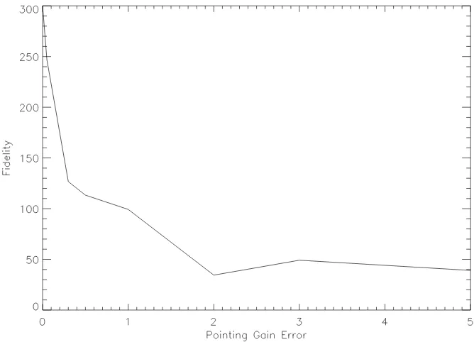
2.7 Fidelity plotted against the gain error equivalent of the actual pointing error . . . 33

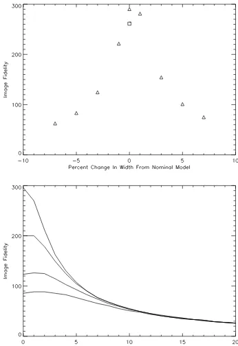
2.8 Image fidelity plotted as a function of error in the assumed beam width 35 2.9 Image fidelity plotted versus ellipticity of the primary beam . . . 36

3.1 Example of how aperture plane illumination offsets result in phase across the sky . . . 48

3.2 Correction factor for aperture plane centroid . . . 55

3.3 Holography result for C4 . . . 56

(13)

3.11 Holography result for C12 interpolated and overlaid with adjuster positions 62

3.12 Holography data for the 10-m antennas in the 1-mm band . . . 65

3.13 Voltage pattern plots of the 10-m antennas in the 1-mm band . . . 66

3.14 Ensemble voltage pattern size of the 10-m antennas clipped at 22% . . 72

3.15 Ensemble voltage pattern size of the 10-m antennas clipped at 10% . . 73

3.16 Ensemble voltage pattern size of the 6-m antennas clipped at 22%. . . 74

3.17 Mean, antenna-style based images and azimuthally-averaged profiles. . 76

3.18 Ensemble voltage pattern ellipticity and position angle of the 10-m

an-tennas clipped at 22% . . . 79

3.19 Ensemble voltage pattern ellipticity and position angle of the 6-m

an-tennas clipped at 22% . . . 80

3.20 Sidelobes of the 10-m antenna illuminated by 6-m and 3.5-m antenna

voltage patterns . . . 82

3.21 10-m antenna real voltage pattern side-lobe stability . . . 84

3.22 10-m antenna imaginary voltage pattern side-lobe stability. . . 85

3.23 Overlaid contours from various runs for the real (left) and imaginary

(right) voltage patterns . . . 89

3.24 Plots of amplitude voltage pattern width as a function of elevation for

the 15 CARMA antennas . . . 92

3.25 Plots of real voltage pattern width as a function of elevation for the 15

CARMA antennas . . . 93

3.26 Plots of amplitude ellipticity as a function of elevation for the 15 CARMA

antennas . . . 95

3.27 Plots of real component ellipticity as a function of elevation for the 15

CARMA antennas . . . 96

3.28 Plots of amplitude voltage pattern ellipticity position angle as a function

(14)

angle as a function of elevation for the 15 CARMA antennas . . . 98

3.30 Plots of magnitude of the imaginary voltage pattern as a function of

elevation for the 15 CARMA antennas . . . 101

3.31 Plots of position angle of the imaginary voltage pattern as a function of

elevation for the 15 CARMA antennas . . . 102

3.32 Image and overlaid contours for the real (left) and imaginary (right)

mean voltage pattern for C1 . . . 107

(15)

3.45 Image and overlaid contours for the real (left) and imaginary (right) mean voltage pattern for C14 . . . 113

3.46 Image and overlaid contours for the real (left) and imaginary (right) mean voltage pattern for C15 . . . 114

4.1 Two different frequencies for pointing error . . . 126

4.2 Pointing sky coverage and post-fit residuals for 10-m antennas with the original catalog and methods . . . 130

4.3 Bin optimization simulation plot of bin size compared to average time per star . . . 133

4.4 Pointing sky coverage and post-fit residuals for the 10-m antennas with the new pointing methods . . . 134

4.5 Systematic residuals in the 10-m pointing model . . . 135

4.6 Elevation pointing offset trend for C4 under thermal stress . . . 138

4.7 Elevation pointing offset trend for radio and optical . . . 147

4.8 Systematic trends in the optical to radio offset vector by night for the 6-m antennas . . . 148

4.9 Systematic trends in the optical to radio offset vector by day for the 6-m antennas . . . 149

4.10 Systematic trends in the optical to radio offset vector by night for the 10-m antennas . . . 150

4.11 Systematic trends in the optical to radio offset vector by day for the 10-m antennas . . . 151

4.12 Amplitude vs. time on a baseline with and without optical offset guiding.153 4.13 Optical offset guiding applied pointing updates for an example track. . 154

(16)

guiding . . . 158

5.1 Overview of the NGC 7538 region in the submillimeter . . . 170

5.2 Spitzer 8µm image of NGC 7538 with 108.1 GHz contours overlaid . . 193

5.3 Spitzer 8µm image of NGC 7538 with high velocity 12_{CO(1-0) contours} overlaid . . . 194

5.4 Integrated 13_{CO and C}18_{O emission near the cloud velocity . . . 195}

5.5 Channel maps of narrow-band HCO+ _{. . . 196}

5.6 Multi-resolution and multi-frequency images of NGC 7538S . . . 200

5.7 Comparison of NGC 7538S at different resolutions . . . 201

5.8 C18_{O and continuum images of NGC 7538S at multiple resolutions . . 205}

5.9 C18_{O spectra along a 60}◦ _{position angle centered on NGC 7538Sa . . . 207}

5.10 HCO+_{(1-0) contours overlaid on a NGC 7538S continuum image . . . . 212}

5.11 12_{CO(1-0) contours overlaid on a NGC 7538S continuum image . . . . 213}

5.12 Self absorption profile toward NGC 7538S . . . 215

5.13 Multi-resolution and multi-frequency images of IRS2 . . . 217

5.14 Very high velocity 12_{CO contours overlaid on a IRS1 continuum image} ₂₂₁ 5.15 Zeroth moment contours overlaid on the first moment map color images of high velocity gas from IRS1 . . . 222

5.16 Inverse P-Cygni profile toward NGC 7538-IRS1 . . . 225

A.1 Optical source and fiber are shown mounted to the antenna secondary in preparation for the optical alignment. . . 249

A.2 The opening to the feed horn is shown overlaid with a cross hairs to aid the optical alignment. . . 250

B.1 The optical telescopes of the 10- and 6-m antennas are shown. . . 254

B.2 The optical camera used at CARMA is shown. . . 255

(17)

List of Tables

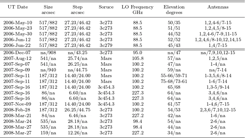
3.1 Holography Data . . . 51

3.2 Adjustment and Alignment Results . . . 59

3.3 Mean Parameters of Antenna Styles . . . 71

3.4 Voltage Pattern Parameters . . . 88

4.1 CARMA Pointing Parameters . . . 124

4.2 Required Limits on the Optical to Radio Offset . . . 142

4.3 Scatter in the Optical to Radio Vector at Night . . . 144

4.4 Scatter in the Optical to Radio Vector by Day . . . 145

5.1 Properties of Young Stars Associated with IRS1-3 and NGC 7538S Com-plexes . . . 171

5.2 NGC 7538 Data Sets . . . 176

5.2 NGC 7538 Data Sets . . . 177

5.3 NGC 7538 Images . . . 184

5.4 Molecular Constants . . . 189

5.5 NGC 7538 Continuum Fluxes . . . 198

5.6 NGC 7538 High Resolution Continuum Fluxes . . . 199

5.7 NGC 7538 C18_{O Fluxes . . . 204}

5.8 NGC 7538 Outflow Properties I . . . 208

5.8 NGC 7538 Outflow Properties I . . . 209

5.9 NGC 7538 Outflow Properties II . . . 210

5.10 NGC 7538 Outflow Properties III . . . 211

(18)

Chapter 1

Introduction

1.1

Into the Mainstream

As both single-dish radio telescopes and radio interferometers have gained in

resolu-tion and sensitivity, the tradiresolu-tional realms of observaresolu-tion–wide field of view, lower

res-olution and high resres-olution, smaller field of view, respectively–have become blended.

Instead of using single-dish observations to map large areas and obtaining

interfer-ometric images to provide detail over single pointings, the advantages of imaging

extended regions with high resolution are becoming evident. New arrays have

re-cently entered into routine function (CARMA1_{) or are under construction (ALMA}2₎

that begin to blur this distinction in the submillimeter regime as well. Both of these

arrays have significantly enhanced sensitivity, resolution, and/or imaging capabilities

when compared to existing arrays while being designed to sample the spatial scales

of sources from the entire region mapped down to arcseconds or less.

Studies of sources with large spatial extent and/or large spatial scales are thus

poised for significant gains. High resolution images (a few arcseconds or less) of

such objects, which include the sun, planets, nearby protoplanetary disks, molecular

clouds within the Galaxy, and nearby galaxies, are rarely achieved in the

submil-limeter regime. The mapping of nearby debris disks has revealed substructures on

several spatial scales (e.g. Corder et al., 2008b; Koerner et al., 2001; Wilner et al.,

(19)

2002). Nearby examples of debris disks may also have large spatial extent (e.g. ǫEri,

Greaves et al., 2005). The dust in these disks is referred to as debris because the

timescale for removal of such dust is much shorter than the age of the systems, i.e. it

must be recreated by collisions (e.g. Backman & Paresce, 1993). Figure 1.1 shows an

example of such a disk, which surrounds the nearby solar analog, HD 107146.

The-oretical models (e.g. Wyatt, 2006) predict that structures in such disks are caused

by resonances with orbiting planets. Planets often inferred from these studies are

typically analogs to the solar system ice giants, a planet population that is not easily

studied, especially at young ages, with any other method. If the planet formation

process is to be understood, a full census of planets at such young ages is necessary.

Such objects cannot yet be imaged at high resolution, a situation higher frequency

observations with ALMA will remedy.

At greater distances, protoplanetary disks have revealed significant substructure.

Figure 1.2 shows the complex morphology of the emission surrounding the young

star AB Aur. The nature of this structure is poorly understood and may be the

result of spiral arms or of infalling envelope material (Grady et al., 1999; Fukagawa

et al., 2004; Corder et al., 2005; Pi´etu et al., 2005). The origin of these features

awaits higher resolution observations with improved sensitivity to disentangle, but

their nature provides vital constraints on the models of young disks and may indicate

that gravitational instability is a valid method of forming massive planets (Boss,

2008). ALMA will observe such objects at very high frequency where the disks will

fill a substantial fraction of the primary beam.

The mass distribution of these protostellar disks is also significant in that it allows

estimates of the lifetimes and typical properties. In particular, the typical mass of

the disks sets limits on which disks are likely to support the formation of planetary

systems. Observations of populations of disks are typically carried out by mosaicing

large areas in dense star forming regions (e.g. Carpenter, 2002; Eisner et al., 2008).

Nearby star-forming regions have been the subject of intense study, but little

work has been done at high resolution over large areas. One of the most important

(20)

[image:20.612.139.503.127.487.2]

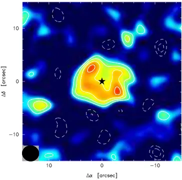
Figure 1.1 1.3 mm continuum emission from the disk surrounding the nearby, solar analog HD 107146 is shown. Contours begin at 2σ and increase by 1σ, where σ is 0.32 mJy beam−1_{. The central region is depressed relative to an asymmetric ring.}

The star indicates the stellar position. The beam is shown in the lower left corner. This image is taken from Corder et al. (2008b).

(IMF). While measurement of this quantity has been studied extensively for stars, it

is unclear whether the stellar IMF is a signature of the distribution of the clumps and

cores from which the stars form or if some evolution has occurred. In the end, it is

the IMF of the clumps and cores that constrain the models of star formation (Enoch,

(21)

[image:21.612.144.501.126.488.2]

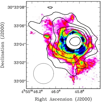
Figure 1.2 The near-infrared scattered light image of Fukagawa et al. (2004) is overlaid with 3 mm, continuum contours from Corder et al. (2005). The contours begin at 3σ, increasing in steps of 2σ=0.72 mJy beam−1_{. The 3 mm continuum beam is shown in}

the lower left corner of the image. This figure was adapted from Corder et al. (2005).

regions. High resolution maps have been obtained (e.g. Testi & Sargent, 1998), but

the field of view is somewhat limited. Wider field images of several such regions at

high resolution are required to determine both the shape of the clump/core IMF and

any environmental variations.

It is often difficult to see the big picture while embedded in the details. For this

(22)

nearby galaxies is the origin and properties of inter-arm H II regions and molecular

clouds. Spurs, substructures associated with the spiral arms themselves and seen in

Figure 1.3, seem to give rise to the inter-arm H II regions (Corder et al., 2008a; La

Vigne et al., 2006). The mere presence of inter-arm molecular clouds has long been

debated. Recent work by Koda et al. (2008) has revealed copious numbers of such

clouds and has determined the apparent mass distribution of these objects, aiding

the understanding of the origin of these clouds, the larger molecular associations

seen in spiral arms, and global star formation. Nearby galaxies like M51 often cover

many square arcminutes on the sky and require large (_∼150 pointing) mosaics. They

also contain a variety of spatial scales with a nearly uniform component covering a

substantial fraction of the disk, linear spiral arm features filling a fraction of the total

area, and point-like molecular clouds populating the inter-arm region.

Arrays like the SMA (Submillimeter Array), CARMA, and ALMA allow efficient

measurement of submillimeter continuum and line emission at several wavelengths at

high resolution. Such multi-wavelength observations are critical. Through the

mea-surement of line ratios, they allow the determination of opacity, temperature, and

spectral indices. The spectral line emission also provides kinematic information.

To-gether, these reveal the physical and dynamical structure of nearly every astrophysical

object. In addition to the objects discussed above, supernova remnants, asymptotic

giant branch stars, and other nebulae contain vital information uncovered through

such ratios.

1.2

Lingering Doubt

From the above discussion, it is clear that submillimeter images of large objects and/or

of large fields of view are critical to several fields of study. However, high dynamic

range is often needed for these observations. The spiral arms of galaxies are bright

while the inter-arm molecular clouds and spiral arm spurs are faint. Weakly emitting

(23)

[image:23.612.143.500.128.485.2]

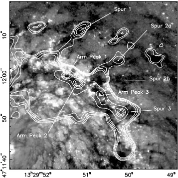
Figure 1.3 Integrated,12_{CO(1-0) emission from M51 is shown as contours on a Hubble}

Space Telescope V-band image. This figure was adapted from Corder et al. (2008a).

protostars. The bright spiral arm-like features or peaks seen in some protoplanetary

disks may dominate the emission from the rest of the disk area. The question becomes

How accurate are the resulting images? If the images are not accurate, the faint end

slope of any mass function or the temperature or the mass density determined by any

image ratio may be more poorly measured than the precision of the measurements

would indicate. The answer to this question is best framed in the study of image

(24)

convolved to the resolution of the observations, to the difference between that model

and an observed map. The image fidelity, in the most general case, is then an image

itself. In practice, various methods are used to determine a single number for the

fidelity that is representative of the average fidelity. In this work, image fidelity is

determined by the peak of the model image, convolved to the resolution of the

ob-servations, normalized by the RMS of the difference between the model and observed

map.

Consider the case of a measurement of the clump/core initial mass function. Due

to the nature of star formation, protostars are often clustered. This is expected to be

the case with natal clumps and cores of protostars as well. A map of a dense, cold

cloud might contain sources with fluxes as bright as 200 to 300 mJy beam−1 _while

also harboring faint clumps with fluxes on the order of 3 mJy beam−1_{, i.e. a ratio}

of 100. Now also assume that the thermal noise in emission-free parts of the map

is <1 mJy beam−1_{. An image of such a region might reveal several faint sources in}

the vicinity of the brightest peak. This may be evidence of clustered star formation.

On the other hand, it may also be the result of poor image fidelity. If the fidelity of

the image in the neighborhood of the brightest peak is on the order of 30, then the

noise limit is better represented by 10 mJy beam−1 _{and the population of faint objects}

should not be considered as they would easily bias the determination of the faint end

of the initial mass function. Therefore, it is clearly not simply the sensitivity limit

which is of importance, but the fidelity as well.

In the above example, fidelity and dynamic range, the ratio of the peak to the

RMS in an image, are interpreted similarly. Now consider a map of a nearby galaxy or

star forming region in which 12_{CO(2-1) and}13_{CO(2-1) observations have been made.}

The ratio of the two lines gives an indication of the opacity. This opacity is then

used to calculate column densities. If the medium is optically thin, then the ratio of

the two lines should be between 40 and 89, depending on the physical conditions in

the region. However, if one of the lines has poor fidelity, then the ratio is improperly

(25)

the mass and any mass moments that are calculated. A similar situation holds for

ratios used to construct spectral indices.

Image fidelity is affected by a variety of factors. For single-dish observations, the

critical limits come from gain and pointing stability. The most fundamental limit

for interferometric observations is the number of samples obtained in the Fourier

plane, i.e. the uv-coverage (Wright, 1999). Therefore, CARMA provides the best

available opportunity for high fidelity, submillimeter imaging to date. CARMA is

a heterogeneous array composed of six 10.4-m (hereafter 10-m) antennas and nine

6.1-m (hereafter 6-m) antennas.3 _{The 105 simultaneous baselines exceeds other}

facil-ities by factors of 3.5 or more.4 _{CARMA achieved first light in August of 2005 and}

has entered into routine function over the last three years.5 _{Two significant}

compo-nents of that commissioning effort are discussed in Chapters 3 and 4. The CARMA

bands are specifically well suited for observing emission from cold dust and

molecu-lar lines. Shorter wavelength bands prove significantly more problematic because of

increased attenuation by the atmosphere and increased difficulties with tropospheric

phase noise.

The heterogeneous nature of CARMA will eventually grant additional benefits

via a unique method of increasing the uv-coverage. The 3.5-m and 6-m antennas can

be placed at separations significantly less than 10 m. This allows observations using

the 10-m antennas as single-dish telescopes, which measures the flux distribution on

angular scales from the entire region toλ/10400, where λ is in millimeters. However,

the limits to image fidelity are restricted by far more than incomplete Fourier coverage.

Due to more stringent constraints on array performance, high fidelity in mosaiced,

interferometric observations is significantly more difficult to achieve (Cornwell et al.,

1993; Wright, 2004, 2007). In the near future with ALMA, a significantly larger

fraction of projects will be limited by image fidelity because the sensitivity will be

greatly increased over any existing facility.

3

At the time of writing, eight 3.5-m antennas of the Sunyaev-Zeldovich Array (SZA) were moved to the location of CARMA and are currently being integrated into the array.

4

The addition of the 3.5-m antennas increases this ratio to nearly a factor of 10.

5

(26)

1.3.1

Basic Assumptions & Equations

Some of the earliest mosaiced, interferometric observations to include single-dish data

to measure the largest scales included M31 and NGC 4258 (Bajaja & van Albada,

1979). Since then, algorithms for improved mosaic deconvolution and

mosaic+single-dish combination have steadily improved. Initially, Ekers & Rots (1979) proposed

that individual pointing centers be used to recover information on spacings in a

neighborhood around the measured baseline, but Cornwell (1988) showed that joint

deconvolution of all the mosaic pointings provides similar recovery. The development

of the maximum entropy methods for joint deconvolution of mosaic and single-dish

observations was also extremely important to the recovery of flux on sources which

have a large range of spatial scales (Narayan & Nityananda, 1986; Cornwell & Evans,

1985). However, the desire for the combined benefits of single-dish telescopes and

interferometric arrays brings with it a host of difficulties. Very few studies have

at-tempted to address the concerns of fidelity with actual data (Wright et al., 1999) or

simulation (Cornwell et al., 1993; Wright, 2004, 2007; Bhatnagar et al., 2008). The

problems inherent in mosaicing along with methods for alleviating these challenges is

the subject of this thesis.

Before embarking on a discussion of the difficulties inherent to mosaicing, it is

important to review the basic equations of interferometry and the typical assumptions

used. The signal, Sx, for an antenna is given by Sx = Ssin(2πνt), where ν is the

observing frequency, S is the input voltage amplitude, and t is time. Now, consider

signals from two such antennas but with the antennas separated by a distance, D,

observing the same source at a position with respect to zenith given by the angle θ.

The product of the voltages is then calculated by the correlator.

The separation of the antennas gives rise to a (geometric) delay in the arrival

of a signal between the antennas, given by τg = Dsin(θ)/c = Dl/c, where c is the

speed of light and l = sin(θ). The product of the signals now becomes SxSy =

(27)

output of F = cos(2πντg)−cos(4πνt)−sin(4πνt) sin(2πντg). The latter terms vary

more rapidly than the first term, cos(2πντg) = cos(2πνDl/c), by several orders of

magnitude in all terrestrial observing conditions and are therefore easily filtered out

(Thompson et al., 2001). The voltage input is thus modulated byF = cos(2πνDl/c),

the fringe function.

Integration of the fringe function over a finite bandwidth, with central frequency

ν0, results in the fringe function evaluated at the bandwidth center modified by a

function with amplitude that falls off with increasingτgor bandwidth. For this reason,

an instrumental delay,τi, is introduced so thatSxSy =S2sin (2πν(t−τi)) sin (2πν(t−

τg)) = S2_F _and _F _≃ _cos₂_πν₍_τ

g −τi)

. The value of τi is then updated to keep

τg −τi small. With this approach, angular offsets, ∆θ, are defined with respect

to the direction θ0, defined where τg = τi, so the fringe function, neglecting the bandwidth function, is cos2πν0(D/c) sin(∆θ) cos(θ0)

. Now, l = sin(∆θ) and u =

ν0Dcos(θ0)/c so that the fringe function, F, is now cos(2πul).

For a source brightness distribution I, the illumination of the source by an

in-terferometer baseline results in an output power, P, given by (e.g. Thompson et al.,

2001):

P(l)_∝ Z

F(l₋l′)P B(l′)H(l′)I(l′)dl′. (1.1) where P B is the baseline primary beam, and H is the bandwidth function. From

the convolution theorem of Fourier transforms, the convolution of two functions is

the same as the product of the Fourier transforms. The Fourier transform of F is

simply the spatial frequency of a given baseline, while the transform of the brightness

distribution, I, is the source visibility function _V. The form of H is typically

well-known.

Now, generalizing to two dimensions, P B is the product of the two, complex

antenna voltage patterns, V1 and V2, that constitute a baseline:

P B(l, m) =V1(l, m)V2∗(l, m) =V1(l, m)V1∗(l, m) =|V(l, m)|2, (1.2)

(28)

Thompson et al., 2001):

V(l, m) =

Z Z _∞

−∞

E(X, Y) exp2πihX λl+

Y λm

i

dXdY, (1.3)

where E is the field pattern in the aperture, X and Y are positions in the aperture,

and m and l are direction cosines on the sky. The field distribution in the aperture

depends on the source distribution and the sensitivity to the structure in the aperture

plane, i.e. it includes any alteration of the source signal from the illumination pattern

and phase response. Typically, a number of assumptions are placed on these voltage

patterns. It is customary to assume that a voltage pattern is real, circularly

symmet-ric, and constant in time. It is also assumed that any gross, time variable, symmetric

introduction of phase or gain error will be removed via astronomical calibration.

AP B for a specific baseline, given in Equation 1.2, modifies the source brightness

distribution described in Equation 1.1, so that the effective brightness distribution

convolved by the interferometer response is actually

I′₍_{l, m}_{) =}_{P B}₍_{l, m}₎_I₍_{l, m}_{) =}_V

1(l, m)V2∗(l, m)I(l, m). (1.4)

Provided the primary beam or constituent voltage patterns are well known, the true

source brightness distribution can be easily recovered by dividing the altered

bright-ness distribution pattern by the primary beam.

1.3.2

Assumptions Violated

In reality, all of the assumptions about the primary beams are not strictly true. The

voltage patterns are very rarely perfectly symmetric, inducing a directional

depen-dence on the sampled brightness distribution. Due to the altitude-azimuth mounts

employed by most telescopes, this symmetry breaking directly implies a time variable

pattern on the sky. The origin of the asymmetries may also change in magnitude and

6_{For CARMA there are different beam patterns but patterns from a given size of antenna are}

(29)

direction with changing physical conditions, specifically temperature and elevation.

Misalignment of the antenna optics can induce phase gradients (to first order) across

the voltage pattern that are also time variable and may depend on observing

condi-tions. The most fundamental of errors in the primary beam, pointing, also induces

this direction, time, and observing condition dependence on the primary beam

pat-tern. Given that the antennas comprising the array are rarely going to have identical

errors, the commonality assumption is also broken. The types of errors in the primary

beam patterns will be elaborated upon in Chapter 2.

Even in the presence of these errors, if precise measurements of the voltage

pat-terns can be obtained, the deviations caused to the attenuated sky brightness

distri-bution can be corrected, although additional procedures are needed (see Chapter 2

or Bhatnagar et al. 2008). That is to say, the deviations of the voltage patterns

from their symmetrized, real, common models are not a problem, but it is the lack of

knowledge of the true voltage pattern which introduces the imaging errors and results

in poor fidelity. However, such complete knowledge is difficult to obtain. Pointing

errors of δl and δm in one antenna cause the source to be illuminated by

I′₍_{l, m}_{) =}_{P B}₍_{l, m}₎_I₍_{l, m}_{) =}_V

1(l−δl, m−δm)V2∗(l, m)I(l, m) (1.5)

instead of by Equation 1.4. When the final image is made, the synthesized image is

divided by the voltage patterns as though the pointing error were not present.

Pointing is a particularly problematic source of primary beam error with respect

to image fidelity. It causes the largest deviations from the assumed pattern at typical

error levels. It is also varies most rapidly. Other types of error, e.g. ellipticity or

beam size errors, introduce additional reductions to the image fidelity, but typically

these are less significant. The decrease in fidelity caused by imaginary components

(30)

It is clear that improvement can be made to image fidelity by exploring the effects of

the relaxation of standard assumptions about the primary beam and comparing the

quantities which result in significant fidelity degradation to the measured deviations

in a functioning system. To this end, we have conducted the following studies:

• Chapter 2: Simulations: Simulated observations are carried out to de-termine the magnitude of the reduction in image fidelity as a function of the

deviation from standard primary beam model assumptions. A limited range

of source models are considered which represent many of the typical observing

situations described above. The simulations reveal that highly deviant

sur-faces, offset illumination patterns, and pointing errors are the leading causes

of fidelity reduction. A method for utilizing the individual voltage patterns to

correct observations is presented.

• Chapter 3: Holography: The surface accuracy of the CARMA dishes was measured. The surfaces were adjusted and the optics were aligned, resulting

in significant improvement on the most deviant antennas. Once completed,

peated measurements of the voltage pattern on the sky revealed consistent,

re-peatable, and significant telescope-to-telescope variation in the voltage patterns

implying that the imaging approach discussed in Chapter 2, which accounts for

the independent voltage patterns, will likely improve the image quality.

• Chapter 4: Pointing: At the time of observation, the leading, correctable cause of fidelity degradation is pointing error. To improve the quality of

point-ing at CARMA, we created a new optical catalog which contains uniform sky

coverage down to the magnitude limit of the current CARMA optical cameras.

The data collection routines were modified to utilize the new catalog and

de-crease the measurement time per source. The new approaches resulted in nearly

a factor of four improvement in the data collection rate. The resulting fits to

(31)

of two. The method was extended to utilize the optical cameras for use during

science observations first at night and then, through new software development,

by day. The resulting decrease in pointing error during a science track was

sub-stantial. This method, called optical offset pointing, is currently used in most

science observations at CARMA.

• Chapter 5: Application to NGC 7538: The new pointing routines, when possible, were applied to observations of the nearby massive star-forming region

NGC 7538. The complex morphology of the region demands reasonably high

image fidelity. It is compact, making it possible to mosaic a substantial fraction

of the region in relatively few pointings. Spectral line and continuum

observa-tions were conducted. The methods of utilizing the measured primary beams

were employed for a few pointing positions to determine if the dominant source

of error in the images was primary beam errors or some other effect like delay or

calibration errors. The high resolution, high fidelity images allow the

identifica-tion of many outflow sources and associaidentifica-tion of these outflows with their driving

source, the measurement of accretion rates directly from absorption profiles and

outflow masses, and the resolution of the dense core NGC 7538S. In turn, these

(32)

Backman, D. E., & Paresce, F. 1993, Protostars and Planets III, 1253

Bajaja, E. & van Albada, G. D. 1979, A&A, 75, 251

Bhatnagar, S., Cornwell, T. J., Golap, K., & Uson, J. M. 2008, A&A, 487, 419

Boss, A. P., ApJ, 677, 607

Carpenter, J. M. 2002, AJ, 124, 1593

Corder, S. A., Eisner, J. E., & Sargent, A. I. 2005, ApJ, 622, L133

Corder, S. A., Sheth, K., Scoville, N. Z., Koda, J., Vogel, S. N., & Ostriker, E. 2008,

ApJ, accepted

Corder, S. A. et al. 2008, ApJ, submitted

Cornwell, T. J. 1988, A&A, 202, 316

Cornwell, T. J. & Evans, K. F. 1985, A&A, 143, 77

Cornwell, T. J., Holdaway, M. A., & Uson, J. M. 1993, A&A, 271, 697

Eisner, J. A., Plambeck, R. L., Carpenter, J. M., Corder, S. A., Qi, C., & Wilner, D.

2008, ApJ, 683, 304

Ekers, R. D. & Rots, A. H. 1979, Image formation from Coherence Functions in

Astronomy, Schoonveld, ed. Reidel, Dordreccht, p 61

Enoch, M. L. 2007, Ph. D. Thesis, Molecular clouds and star formation: a

multiwave-length study of Perseus, Serpens and Ophiuchus

Fukagawa, M. et al. 2004, ApJ, 605, L53

Grady, C. A., Woodgate, B., Bruhweiler, F. C., Boggess, A., Plait, P, Lindler, D. J.,

(33)

Greaves, J. S. et al. 2005, ApJ, 619, L187

Koerner, D. W., Sargent, A. I., & Ostroff, N. A. 2001, ApJ, 560, L181

Koda et al. 2008, Nature, submitted

La Vigne, M. A., Vogel, S. N., & Ostriker, E. C. 2006, ApJ, 650, 818

Pi´etu, V., Guilloteau, S., & Dutrey, A. 2005, A&A, 443, 945

Narayan, R. & Nityananda, R. ARA&A, 24, 127

Thompson, A. R., Moran, J. M., & Swenson, G. W. 2001, Interferometry and

Syn-thesis in Radio Astronomy, New York, Wiley-Interscience

Testi, L. & Sargent, A. I. 1998, ApJ, 508, L91

Wilner, D. J., Holman, M. J., Kuchner, M. J., & Ho, P. T. P. 2002, ApJ, 507, L115

Wright, M., Dickel, J., Koralesky, B., & Rudnick, L. ApJ, 518, 284

Wright, M. C. H. 1999, BIMA Memo Series 73

Wright, M. C. H. 2004, CARMA Memo Series 27

Wright, M. C. H. 2007, CARMA Memo Series 38

(34)

Chapter 2

Simulations: Limitations on

Dynamic Range and Image

Fidelity For Wide Field Imaging

Abstract

Here we present simulations that include the effects of relaxing many typical

assump-tions about the interferometer primary beam on image fidelity. The degradation of

image fidelity as a function of errors in pointing as well as errors in the assumed

properties of the primary beam are simulated, allowing for heterogeneity among the

constituent beams. Critical characteristics that must be corrected to some degree

be-fore high-fidelity imaging can be achieved include surface accuracy, optical alignment,

and pointing. Once these deviations are addressed, a more accurate model of the

pri-mary beam shape is required to further improve fidelity. Using these simulations, we

propose a method of correcting for deviant primary beams in real observations.

2.1

Introduction

The concepts of high image fidelity and dynamic range were provided in Chapter 1

along with their implications for scientific observations. A variety of factors can,

however, restrict image fidelity. Some of these, including poor sensitivity,uv-coverage,

(35)

and atmospheric phase noise, can be attributed to the inherent properties of the array

being used. Others arise from more systematic errors such as baseline solutions,

improper primary beam models, or instrumental gain variation.

Foremost among the inherent limitations is the fact that interferometers sample

finitely many spatial scales. Consider, for example, the measurement of the visibility

VS(~u) = K X

k=1

δ(~u₋~uk)_V(~u) (2.1)

where_VS _{is the measured visibility function,}_V _{is the Fourier transform of the source}

flux distribution, i.e. the visibility function, δ is the delta function, and the points

~uk (the uv-coverage) are the finite positions of measurement for the observation. In

reality, the visibility function is averaged over a patch of uv-space of width ~u_±d,

where d is the antenna diameter.

In the neighborhood of uv-points actually measured, i.e. over the range ~u_±δ~u,

some information can be recovered by the deconvolution process by making

assump-tions about the source extent (Cornwell, 1988), by inverting with respect to

individ-ual pointing centers (Ekers & Rots, 1979), or by use of Cauchy relations to constrain

derivatives in the complex plane. Also, mosaicing observations allow recovery of

infor-mation initially lost in averaging over the finite size of the antennas in use (Thompson

et al., 2001).

However, the interferometer cannot sample the visibility function everywhere. The

effect of this limitation is greatest in cases where there are few antennas in the array

or where large regions requiring multiple pointings are observed. In the former case,

the number of baselines sampling theuv-plane is inherently sparse. In the latter, the

size of the region impacts the density of sampling of the uv-plane associated with

individual patches of sky. In principle, repeated observations can fill in the uv-gaps

generated by multiple pointings, but in practice this is extremely complicated and

source size inevitably limits image fidelity (Wright, 2007).

Arrays like CARMA, with a significant number of antennas and thus dense uv

(36)

nevertheless limited by the inability to sample the central region of theuv-plane due

to the finite physical size of the antennas. This central region of the uv-plane is

associated with the largest angular scales in the map, scales which may contain the

vast majority of the flux. On the other hand, heterogeneous arrays, like CARMA, offer

a unique opportunity to overcome this limitation using the larger antennas to recover

flux on the largest angular scales. In principle, there is no need to utilize smaller

telescopes to bridge the uv-gap (Cornwell et al., 1993), but, in practice, overlap aids

the relative calibration. A value of two (e.g. Thompson et al., 2001) is often quoted for

the necessary ratio of large diameter antenna to smaller diameter antenna to obtain

sufficient overlap, although a slightly smaller ratio is likely tolerable.1

Further limits to image fidelity exist. Array sensitivity limits fidelity since weak,

but real, structure in a map cannot be accurately recovered. Atmospheric phase noise,

causing preferential smearing of the smallest structures in the map, will also have an

adverse effect on fidelity. These limitations are, at present, unavoidable, although

efforts are being made to reduce such phase errors via comparison with phase

fluctu-ations in the water line (water vapor radiometry) and the use of additional antennas

to follow the phase on nearby quasars at lower frequencies. Other detriments to

im-age fidelity arise from random and systematic effects that are, in principle, avoidable

or at least can be minimized. Among these, imperfect knowledge of the primary

beam presents the largest, correctable barrier to obtaining high-fidelity observations

of extended objects (Cornwell et al., 1993).

Theoretical arguments and basic simulations that have been used to date to

pro-duce estimates of fidelity degradation in the presence of primary beam model error

suffer from two fundamental limitations: they assume circular symmetry of the

pri-mary beams and they treat the antennas as identical entities. In reality, errors such

as a misaligned illumination pattern on the antenna surface, sidelobes, off-axis focus

error, or ellipticity in the primary beam result in significant deviations from

sym-1_{The limiting factor is imposed by the taper of the illumination pattern on the constituent}

(37)

metry. Since these systematic deviations are rarely uniform across all the antennas,

the antennas cannot be regarded as uniform entities. Indeed, pointing errors alone

result in the non-uniformity of antenna primary beams. The deviations among

anten-nas result in decidedly different performance and may reduce fidelity in final image

reconstruction.

More careful simulations can provide both quantitative measures of the decay

of fidelity as a function of various parameters for different models and qualitative

representations of the resulting changes in image appearance. However, to date, many

difficult parameters have been simulated using simplifying approximations for errors.

Specifically, pointing error has been simulated using gain error. Gain errors affect

the fidelity by scaling the overall flux response. True pointing and primary beam

error affect the image differentially, resulting in gradients across the illuminated sky

relative to the assumed illumination.

Here, we present a suite of simulations encompassing various departures from

the standard primary beam assumptions. While these simulations are specific to

CARMA, the methods are easily generalizable to any array. In practice, the degree of

fidelity decay is highly dependent on the exact source structure. We focus on

situa-tions where fidelity and dynamic range are likely to be of concern. These simulasitua-tions,

in turn, motivate corrective methods for use in real-time (described in Chapters 3

and 4) and in data processing (described in Chapter 5). Source models and the

vari-ables are discussed in_§2.2, while the simulations are outlined in_§2.3. The simulation

results are presented in _§2.4 and discussed in _§2.5. Conclusions and suggestions for

future work are in _§2.6.

2.2

Models & Variables

Three general models are considered here. Point source and resolved Gaussian source

models represent a large fraction of typical observations with interferometers and

have rather simple structure. The third model, shown in Figure 2.1 at the scale used

(38)

reasonable approximation for extended2 _{sources such as nearby galaxies, supernova}

remnants, some debris disks, and asymptotic giant branch stars. In the case of Cas A,

the integrated flux of the map is over 700 Jy and the peak flux is _∼10 Jy. This rather

large flux ensures that the simulations are truly in the fidelity limited regime, since

typical thermal noise in a single, mosaiced, continuum track at CARMA is a few mJy.

The Cas A model shown in Figure 2.1 has significant flux out to 100-m baselines,

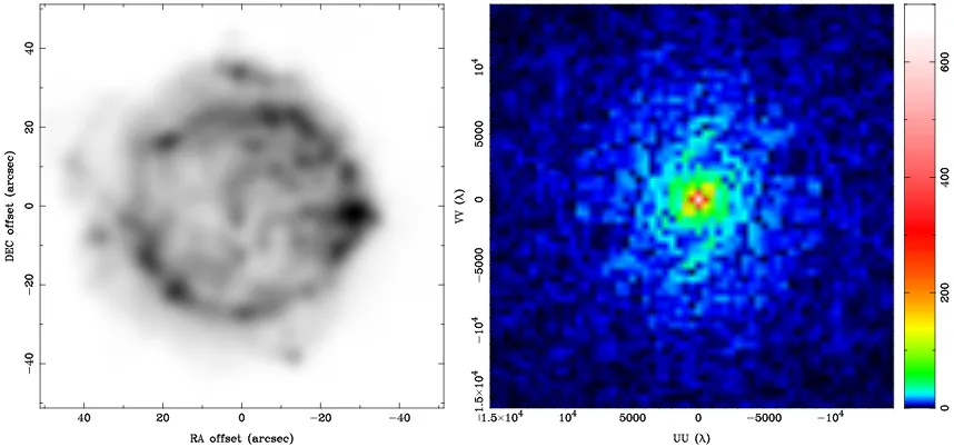
[image:38.612.108.537.308.509.2]

showing that the source indeed has flux on a variety of spatial scales.

Figure 2.1 The model is a C-band image of the supernova remnant, Cas A. The left panel shows the source scaled to cover a region comparable with the FWHM of the 10-m primary beam. The right panel shows the flux amplitude of the model in the Fourier plane with the pixel scale in Janskys. The axes in the right panel are in units of λ=2.6 cm.

In reality, it is not errors in the primary beam which are a problem but, more

specifically, deviations of the assumed primary beam from the actual one which

de-grade fidelity. In these simulations, the assumption is that arealisticprimary beam is

2_{In this context, an extended source is one whose spatial extent is comparable to or larger than}

(39)

used to illuminate the source on the sky and then the assumed, model primary beam

is used in the imaging process. Image fidelity is affected by other systematic errors

as well, but most of these errors are introduced by more fundamental limitations in

the array performance.

The primary beam is the product of two, antenna-based, complex voltage patterns

given by Equation 1.2. The measured visibility function, _VM₍_~u₎3 _{is related to the}

voltage patterns, V, through

VM(~u)_∝ Z ∞

−∞

Vi(~k)Vj(~k)I(~k)e−2iπ( ~_k_·_~_u₎

d~k, (2.2)

where I is the source brightness distribution and the bandwidth function has been

ignored since it is assumed to be well known. If one or both of the voltage patterns

differ from the assumed model, then Vi(~k) must be replaced by some altered voltage

pattern, V′

i(~k). However, since Vi(~k) is still used in the final image construction process via the primary beam, errors in the voltage patterns can adversely affect the

measured visibilities and the primary beam correction during the image restoration

process.

At the most basic level, deviations from the ideal primary beam are caused by

errors in the antenna surfaces that in turn reduce forward gain. While the antenna

gain can be measured relatively precisely, flux scattered by small scale imperfections

in the antenna surface pollutes the image with a scattered beam outside the main

beam. The scale of such deviations is typically a fraction of a wavelength (_≤100µm at

millimeter wavelengths), and not systematic for well functioning millimeter telescopes

(see Chapter 3). Since it is extremely difficult to model such small scale variations,

these errors can be approximated by gain errors, δG = 1₋exp(₋[4πσ/λ]2_{) where} _σ

is the surface accuracy and λ is the observing wavelength (Ruze, 1966). This

repre-sentation for the error assumes that the surface/phase errors are Gaussian random

numbers which are distributed evenly over the aperture and that the correlation size

3_{This is to distinguish between the visibility function altered by the illumination patterns, the}

true visibility functionV, and the visibility function that arises from the finite sampling of the array,

(40)

error, the resulting gain errors are 1.6% and 8.0% at 3 mm and 1.3 mm, respectively.

The next order of primary beam error is simply due to uncertainty in the assumed

center of the primary beam, i.e. a pointing error. Consider the case of two, 1-D

Gaussian patterns, of widths and σ1 and σ2, and one of the patterns is perfectly

pointed while the other is offset by µ, the resulting primary beam has widthσ2

new =

σ2

1σ22/(σ12+σ22), center µnew =µσ12/(σ21 +σ22), and peak

A= exp−µ

2

2σ2 2

h

1₋ σ

2 1

σ2 1 +σ22

i

, (2.3)

where in the limit of σ1 = σ2 = σ these reduce to σnew2 = σ2/2, µnew = µ/2, and

A = exp (₋(µ/2σ)2_{). For a pair of 10-m antennas, the forward gain is reduced by}

1% for antennas offset by 5′′ _{but reaches 5% by a 11.5}′′ _{offset. For 6-m antennas, the}

same 11.5′′ _{error results in a 2% gain error.}

It is worth noting that for sources of any finite extent,4 _{pointing error does more}

than reduce the forward gain. The extension of the source and the offset location

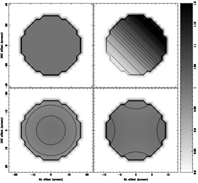
of the beam center results in a differential effect, as demonstrated in Figure 2.2. A

comparison of the upper left and right panels shows the impact of an illuminating

beam offset from the true center for a disk model. The errors in the flux reach

±25% at the edge of the disk and are distributed as a linear gradient. The pointing error assumed for this model is within 2 standard deviations of the nominal pointing

position based on the repeatability of CARMA pointing offsets (see Chapter 4).

As will be described in detail in Chapter 3, the correct width and shape of the

primary beam can be established from detailed measurements of the beam on the sky.

In practice, current software imaging packages utilize circularly symmetric profiles for

the primary beams. MIRIAD, the default imaging package for CARMA, currently

uses a circularly symmetric Gaussian profile for the CARMA primary beams. Errors

can be introduced if the size of the profile differs from that assumed in the model. The

bottom-left panel of Figure 2.2 shows that this effect results in a quadratic variation

4_{The use of extended is avoided here as the effects to be discussed apply to sources of any}

(41)

[image:41.612.125.522.127.494.2]

Figure 2.2 The top-left panel shows a uniform disk where the beam used to illuminate the source was also used to correct the final image. The top-right panel shows a primary beam offset by 8% of the FWHM from the nominal pointing location. The bottom-left panel shows the disk restored with a primary beam 3% different in size from the beam model. The bottom-right panel shows the disk illuminated by a beam which has an ellipticity of 3% but of the same size as the beam model. The model disk has unit flux per pixel and is equal to the size of the FWHM of the beam in question. The pixel scale ranges from 0.8 to 1.2. The contours also span 0.8 to 1.2, initially in steps of 0.05. Inside 0.95 and 1.05, the contours are in intervals of 0.02.

across the disk with perfect agreement at the beam center and growing deviation

towards the edges. The errors induced, however, are relatively small when compared

(42)

of the profile from a Gaussian. The true shape of the beam compared to a Gaussian

profile is discussed in detail in Chapter 3. In general, the beam profile appears to

be flatter (i.e. wider) in the beam core compared to a Gaussian but steeper (i.e.

narrower) than the Gaussian profile in the wings.

To a lesser extent, errors can result from slight deviations from circular symmetry

even when the adopted primary beam size is correct. This ellipticity is defined ase =

amajor/aminor, where amajor and aminor are Gaussian fits to the FWHM of the beam

profile. The bottom right panel of Figure 2.2 shows the influence of 3% ellipticity

(e = 1.03). Here the error pattern is quadrupolar in shape. Several methods of

introducing ellipticity can be envisioned. A common ellipticity for a given antenna

style, i.e. all 6-m antennas and all 10-m antennas, with a position angle of 0◦ _could

be used. Or, the ellipticity could remain fixed on antennas of a common diameter

but the position angle of the ellipticity could vary. Finally, an independent ellipticity

and position angle on an antenna basis may arise.

Sidelobes can also be asymmetric. The primary beam of the heterogeneous

base-lines at CARMA is formed by the geometric mean of the primary beams from the

con-stituent antennas. The low-level sidelobes of the 10-m primary beam are multiplied

by higher power points in the 6-m primary beam, resulting in increased sidelobes.

Measurement of the ellipticity, departures from Gaussian profiles, and sidelobe

patterns are, in practice, quite difficult. In particular, the ellipticity and sidelobe

patterns of the profile can change appreciably with elevation and temperature. A

long-term campaign to monitor the primary beam profiles would be necessary to say

with certainty that a systematic ellipticity is present or that sidelobe patterns are

consistent. Even then, determination of the true primary beam profile would require

further observations to average over temporal changes and noise in the inherently less

sensitive portions of the beam which typically harbor the deviations.

In addition to any departures from Gaussian profiles, it should be noted that the

elements of an array can differ from each other. In reality, CARMA, or any other

array, is not an array ofN+ N₂

(43)

of distinct antenna types; it is an array of M₂

different primary beams whereM is the

number of antennas, i.e. M independent voltage patterns form independent primary

beams on a baseline basis. These antenna voltage patterns might have different

sizes, ellipticities, pointing offsets, and even imaginary components. In the limit of

common antenna voltage patterns for all antennas, the imaginary components of the

beam cancel perfectly in the imaginary beam but these components can give rise to

ellipticity in the real component.

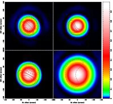
If patterns differ, as they in fact do for every antenna in every array, the imaginary

components may seriously influence the image fidelity. The panels of Figure 2.3 show

examples of baseline-based, homogeneous and heterogeneous primary beams from

CARMA. The top panels show the primary beams for a pair baselines composed

en-tirely of 10-m antennas, hereafter a 10-m baseline. On the left, the constituent voltage

patterns have imaginary gradients in opposite directions resulting in an amplified

gra-dient of +20% to -15% across the image. On the top-right, the contributing voltage

patterns have small imaginary components and thus have peak imaginary components

of 6%. The bottom left panel shows a heterogeneous baseline where the 6-m antenna

voltage pattern is imaginary component-free, but it illuminates a 10-m antenna

volt-age pattern which has a significant imaginary component so the gradient persists.

The bottom right panel shows a primary beam from a baseline composed of two 6-m

antennas, hereafter a 6-m baseline, which are largely free of imaginary contribution.

In all, these four examples demonstrate that the assumption of uniformity is far from

valid.

2.3

Simulations

All simulations are conducted using MIRIAD (Sault, Teuben, & Wright, 1995),

wrapped within Python and supplemented with IDL to perform free rotations of

the beams to arbitrary parallactic angle.5 _{Simulations are carried out at 100.2 GHz}

5

(44)

[image:44.612.125.523.126.492.2]

Figure 2.3 A variety of measured real (color) and imaginary (contour) primary beams are shown for a heterogeneous array. The first two contours are at 3% and 5% and then contours increase by 5% thereafter. Negative contours are shown as dashed lines. The top panels display primary beams from 10-m baselines. The bottom left panel shows the primary beam from a heterogeneous baseline while the bottom right shows a 6-m baseline primary beam.

since the true voltage patterns are measured at this frequency (see Chapter 3). It

is easy to scale the frequency of the templates used by changing the cell size in the

voltage pattern by a factor of the ratio of the frequencies. Only the influence of gain

and primary beam error are addressed here, although the simulation package includes

(45)

For the purposes of these simulations, only the CARMA “D” configuration, which

gives a resolution of 4-5′′_{in the 3-mm band, is used. Nyquist sampled pointing offsets}

for mosaics are used for all simulations. Observations of Cas A consisted of a seven

pointing mosaic. Simulated observations span 4 hours centered about transit. A

variety of metrics are required to assess the resulting image quality. The basic metric

for the simulations will be fidelity, defined as the ratio of the peak flux of the model

at the simulation resolution and RMS of the residual image. For Gaussian and point

source models, fits to the image profile are also used to determine the quality of the

simulated observations.

Simulations begin by separating the specified observing time into subsets since

asymmetric beam patterns or real pointing errors require a time evolving pattern.

Over the specified time range, uv-data for an empty field is generated using uvgen,

which requires information on antenna performance, configuration, and mosaic

pat-tern, as well as the location of the source to be used in the simulation. The average

parallactic angle of the model source is then retrieved from the generated dataset.

For each pointing location in the mosaic pattern and antenna pair, the model image

is multiplied by the product of two offset voltage patterns resulting in, for the most

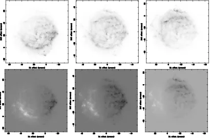
general case, a real and imaginary brightness distribution. Figure 2.4 shows various

primary-beam-illuminated pointings of the Cas A model.

Once the baseline-specific, single-pointing, primary-beam-illuminated model is

available, the image is fed to uvmodel, using the output of uvgen as the

base-line visibility file. This produces a file which adds the noise of the original visibility

file to the visibilities of the model sampled at the values given by uvgen. First the

real component is sampled, then the result is fed to uvmodel again, now using the

imaginary component of the brightness distribution and the optionimaginary, which

permutes the components and changes sign for proper complex algebra.

Gain error is introduced as a percentage of the antenna gain, nominally 1.0. The

amplitudes of the simulated visibilities are multiplied by an antenna based quantity,

independent for each antenna, that has a

Optimizing Image Fidelity with Arrays

Stuartt A. Corder

Abstract

Contents

List of Figures

List of Tables

Chapter 1

Lingering Doubt

Basic Assumptions & Equations

Assumptions Violated

Chapter 2

Introduction

Models & Variables

Simulations