DOI: 10.1017/S095679250300531X Printed in the United Kingdom
639
Similarity solutions to an averaged model for
superconducting vortex motion
G. R I C H A R D S O N
Section of Theoretical Mechanics, University of Nottingham, Nottingham NG7 2RD, UK
(Received 27 March 2002; revised 27 May 2003)
Under certain conditions the motion of superconducting vortices is primarily governed by an instability. We consider an averaged model, for this phenomenon, describing the motion of large numbers of such vortices. The model equations are parabolic, and, in one spatial dimensionx, take the form
H2t=
∂
∂x(|H3H2x−H2H3x|H2x), H3t=
∂
∂x(|H3H2x−H2H3x|H3x).
whereH2 andH3are components of the magnetic field in theyandzdirections respectively. These equations have an extremely rich group of symmetries and a correspondingly large class of similarity reductions. In this work, we look for non-trivial steady solutions to the model, deduce their stability and use a numerical method to calculate time-dependent solutions. We then apply Lie Group based similarity methods to calculate a complete catalogue of the model’s similarity reductions and use this to investigate a number of its physically important similarity solutions. These describe the short time response of the superconductor as a current or magnetic field is switched on (or off).
1 Introduction
region along vortices, has been termed the mixed state because there is no large-scale separation of normal and superconducting phases as in a Type-I superconductor.
Many models have been proposed to describe the behaviour of superconductors. One of the most successful of these is the so-called Ginzburg–Landau model [17], which describes the behaviour in terms of two variables, the magnetic field H and an order parameter
ψ, the modulus of which is related to the local density of superconducting electrons. Reviews of the mathematical aspects of this model are given in Chapmanet al. [10] and Duet al. [13]. Its most notable triumph was the prediction of vortices by Abrikosov [1]. An important feature of the model is that the morphology of solutions is found to be crucially dependent on a certain material parameter, the Ginzburg–Landau parameterκ, which gives the ratio of typical variations in the magnetic field (the penetration depthλ) to typical variations in the order parameter (the coherence length ξ). In particular, the value of κ determines whether Type-I (κ < 1/√2) or Type-II (κ > 1/√2) behaviour is exhibited. Here we shall be interested in the high-κlimit in which the thickness of the core of the vortex, outside which the size of the order parameterψ does not vary appreciably, tends to zero. For a large number of materials, typically alloys, this limit provides a good description, examples being NbSn,κ= 15.3; NbNi,κ= 28.0 and V3G,κ= 25.3.
The macroscopic response of a Type-II superconductor to changes in the surrounding magnetic fields is primarily governed by the motion of large numbers of superconducting vortices. Furthermore vortex motion within the superconductor leads to energy dissipation which in many applications is undesirable. Vortex motion may be retarded by introducing impurities into a superconducting material; these act to trap vortices and this effect is termedpinning(see, for example, Chapman [7]). So-called critical state (stick-slip) models are widely accepted as providing a good description of the long-timescale behaviour for vortex motion in two-dimensional geometries (see Bean [2] and Chapman [7]). However, there remain unresolved issues in the extension of these models to fully-three dimensional geometries with several candidate models in existence [12, 5, 7]. In this work, we shall be interested in vortex motion in the absence of pinning, but note that the physics of vortex flow in pinned superconductors is essentially the same as in un-pinned materials and so our work has potential applications to devices such as fault-current limiters in which the pinning potential is exceeded and an unretarded vortex flow occurs. Furthermore the correct formulation of a three-dimensional critical state model (for pinned superconduct-ors) requires that the short-time scale flow of vortices is properly understood, and in this respect, we expect this work will further understanding.
Vortices move in response to their curvature and gradients in the magnetic field (electric currents). In the limit asκbecomes large, and in the absence of vortex pinning, the vortices move with velocityvwhere
β
2v=
Clogκ
2 n+ (∇ ∧H)∧t. (1.1)
current on the vortex – this is often termed the motion due to the Lorenz force. The problem for vortex motion is coupled to a problem for the magnetic fieldH,
∇ ∧(∇ ∧H) +H= 2π
n
k=1
δΓk(x), (1.2)
where the summation is over all the vortices present in the superconductor, Γk is thekth vortex curve and
δΓk(x) =
Γk
δ(x−xˆ)δ(y−yˆ)δ(z−zˆ)dxˆ.
In practice, it is not feasible to use this model directly to simulate the response of a macroscopic superconducting sample because of the vast number of vortices typically found inside such samples. This has led to the search for an averaged model of supercon-ducting motion which is capable of giving an approximate description of the motion of large numbers of vortices. Modelling of this form was first conducted by Brandt [5] on the basis of heuristic arguments. A subsequent formal derivation of an averaged model from (1.1)–(1.2) was made by Chapman [6] in a regime where vortices are sufficiently densely packed, and the magnetic fields correspondingly large, so that the the first term on the right of (1.1) can be neglected. In certain special geometries, such as thin films, this turns out to be a reasonable assumption however in most three-dimensional situations such an assumption leads to a model which is linearly ill-posed [20]. The reason for this pathological behaviour is a three-dimensional vortex instability that occurs wherever there is a component of ∇ ∧H in the direction of the vortex tangentt; this instability was first noted by Clem [11]. Over a short time scale, the instability causes vortex lines to develop a highly curved spiral structure which invalidates the assumption that the second term on the right-hand side of (1.1) is much larger than the first. A more detailed investigation, carried out in earlier work [18], reveals that the instability grows so as to try to align the vortex tangent perpendicular to the local electric current densityj=∇ ∧H or, taking an alternative viewpoint, that the resulting vortex motion causes an electric field parallel to the current densityj.
The implications of the evolution of this instability has been considered by Chapman & Richardson [9], who proposed a model for the evolution of large numbers of vortices in a superconductor without pinning. For more details on the derivation and the regime of validity we refer the reader to Chapman [7]. Here we shall be content with writing down the model and some brief explanation. The long wave limit of the model (see equations (5.9)–(5.11) of Chapman [7]), which describes the evolution over lengthscales much greater than the penetration depth of the material (typically about 10−7m) is, in dimensionless
variables,
∇ ·H= 0, (1.3)
Ht+∇ ∧E=0, (1.4)
j=∇ ∧H, (1.5)
E=δH∧
j∧ H |H|
+|j·H|j. (1.6)
field from the Lorenz force, while the second represents the contribution from the vortex instability and δ is the ratio between these two contributions. In the regime of validity of this model (the vortex fluid regime) δ is small.1 In addition to modelling clean
superconductors (which have no vortex pinning sites) this model also has applications to vortex flow in superconductors with pinning since, once the pinning potential has been overcome, the flow of vortices obeys the same physics as that for a clean superconductor. It can thus be used to describe vortex flow in devices, such as a fault current limiter, which are designed to give significant flows under certain conditions.
This is the first analysis of this model and, in order to make progress, we limit our investigation to the simplest geometry in which non-trivial solutions to the model can be found. This is the one-dimensional slabα < x < β which models a superconducting sheet, or tape. Furthermore, we assume this slab is subjected to a parallel applied magnetic field Happland carries a transport currentItransper unit length which flows in they-zdirection. With this in mind we look for solutions of the form
H = (0, H2(x, t), H3(x, t)),
and on substitution into (1.3)–(1.6), we find
H2t =
∂
∂x(|H3H2x−H2H3x|H2x) +δ
∂ ∂x
H2
(H2H2x+H3H3x)
H2 2+H32
1/2
, (1.7)
H3t =
∂
∂x(|H3H2x−H2H3x|H3x)) +δ
∂ ∂x
H3
(H2H2x+H3H3x)
H2 2+H32
1/2
. (1.8)
Sinceδ is small, we neglect terms involvingδ and solve instead the simplified system
H2t=
∂
∂x(|H3H2x−H2H3x|H2x), (1.9) H3t=
∂
∂x(|H3H2x−H2H3x|H3x). (1.10)
The resulting equations form a parabolic system. Boundary data of the form
(0, H2, H3) =H− on x=α, (0, H2, H3) =H+ on x=β, (1.11)
must be supplied together with initial conditions forH2 andH3. The boundary data for
this problem comes from specifying the applied magnetic field Happl and the transport currentItrans, and is found from the relations
H++H−= 2Happl, H+−H−= (0,Itrans.ez,−Itrans.ey).
Initial conditions are obtained from a knowledge of the initial density of vortices (magnetic field is proportional to vortex density). This model has a high degree of symmetry and a correspondingly large number of similarity reductions. It is, for instance, invariant under
translations in x and int, under rotations of the (H2, H3) coordinate axes and under the
following rescaling:
H2 →qH2, H3→rH3, x→px, t→ p3 qrt,
whereq,r andpare all arbitrary constants. As a result we expect the model to exhibit a large number of similarity reductions.
The aim of the present work is threefold: first, to investigate the steady states to this novel model of supercondcuting vortex motion; secondly, to examine its unsteady behaviour using a numerical scheme; and finally, to derive its similarity reductions and analyse some of its physically pertinent similarity solutions. We now briefly summarise the main results of the first part of the paper. Of particular importance is a steady solution of the form
H2=ax+b, H3=cx+d, (1.12)
wherea,b,candd are arbitrary constants, which describes a state with uniform current density across the width of the superconductor. It is noteworthy that there is exactly one such steady solution for each set of boundary data (1.11) applied to (1.9)–(1.10). We demonstrate that such solutions are stable to small one-dimensional perturbations and this motivates the search for similarity solutions which describe the evolution from one steady state of the form (1.12) to another such steady state as either, or both, of the applied magnetic fieldHappl and the transport currentItrans are impulsively changed. These similarity solutions take one of two forms: the first describes the evolutions from an initially constant magnetic field; while the second describes the evolution from a magnetic field of the typeH2=ax+b,H3=cx+dbut assumes the impulsively changed
boundary magnetic field lies in a particular direction. Both types of solution describe the evolution in a semi-infinite slab (β → ∞) and thus provide the short time behaviour for the evolution in the finite slab. The long-term behaviour of this evolution is provided by the linear stability analysis. There is also another non-trivial steady solution
H3=kH2(x), (1.13)
wherekis an arbitrary constant. However this solution is of less physical interest because (i) it can only ever be realised ifItrans·Happl= 0 and (ii) because, unlike (1.12), neglecting the O(δ) terms in the full problem (1.7)–(1.8) represents a singular perturbation. The preceding facts leads us to conjecture that solutions to (1.9)–(1.10) satisfying steady boundary conditions which have the property Itrans·Happl =H3−H2+−H2−H3+0 decay
to the unique steady solution of the form (1.12) which satisfies these boundary conditions. In §2 we derive all the steady solutions to (1.9)—(1.10); these fall into two classes, the first being of type (1.12). We then investigate the stability of (1.12) to small one-dimensional perturbations before proceeding to look at numerical solutions to the models in §3. In §4 we derive the infinitesimal Lie point symmetries of the model. We then use these and the method of invariant surfaces to construct a complete catalogue of the model’s similarity reductions. In§5 we look for travelling wave solutions. Then in§6 and §7 we investigate similarity solutions which exhibit decay to steady solutions of the from
investigate a subclass of similarity solutions which can decay to steady solutions of the second kind (1.13), and finally draw conclusions.
2 Steady solutions
Looking for steady solutions to (1.9)–(1.10) by substitutingH2=H2(x) and H3 =H3(x)
results in a set of O.D.E.s that we can integrate exactly. Doing so we find thatH2andH3
either take the form
H2=ax+b, H3=cx+d, (2.1)
wherea,b,c, anddare arbitrary constants, or take the form
H3=kH2(x), (2.2)
where k is an arbitrary constant and H2 an arbitrary function of x. Physically, (2.2)
corresponds to a solution for which j·H =|H3H2x−H2H3x| ≡0, whereas solutions of the form (2.1) do not have this property. Thus neglecting theO(δ) terms in the full system of PDEs (1.7)–(1.8) represents a non-singular perturbation when the steady solution is of the form (2.1), and a singular perturbation when it has the form (2.2). In other words if we include the O(δ) terms in (1.7)–(1.8) we find an O(δ) correction to (2.1), whereas we cannot find such a correction to (2.2). In order to work out what happens to such steady solutions to the model (1.9)–(1.10) when we reintroduce the O(δ), terms we look for solutions to (1.7)–(1.8) of the form
H2 =H2(x, τ), H3=kH2(x, τ), τ=δt.
Substitution into (1.7)–(1.8) leads to the following slow timescale equation forH2:
∂H2
∂τ = (k
2+ 1)1/2 ∂
∂x
|H2|
∂H2
∂x
. (2.3)
This is a well known version of the porous medium equation and implies that over long times such solutions evolve towards a profile of the formH2=±(cx+d)1/2, wherecand dare arbitrary constants.
To summarise, if we consider solving for a steady solution in a slab α < x < β and imposing the boundary conditionsH=H−on x=αandH=H+ onx=β, then where H− andH+ have the propertyItrans·Happl=H3+H2−−H3−H2+= 0, there is an infinite set
of possible solutions given by (2.2). However, where this condition is not satisfied there is a unique solution of the form (2.1).
2.1 Linear stability analysis
We now investigate the stability of the steady solution (2.1) by perturbing about it in the following manner:
H2=ax+b+eσtp(x), H3=cx+d+eσtq(x).
We assume thatH2andH3are specified on the boundaries of the body,x=αandx=β,
such that
p(α) =p(β) =q(α) =q(β) = 0. (2.5)
Substituting (2.4) into (1.9)–(1.10) leads, after some manipulation, to the following eigen-value problem:
p− σ
2(ad−bc)|ad−bc|[(ad−2bc−acx)p+ (ab+a
2x)q] = 0, (2.6)
q− σ
2(ad−bc)|ad−bc|[−(cd+c
2x)p+ (2ad−cb+acx)q] = 0, (2.7)
which is supplemented by the boundary conditions (2.5). Note that if ad=bc then we effectively have a solution of the type (2.2) and the preceding long timescale analysis applies so that we need not consider this possibility further. Multiplying (2.6) by cand subtracting (2.7) multiplied bya leads to
Θ− σ
|ad−bc|Θ= 0, where Θ=cp−aq.
Multiplying this equation byΘ, integrating fromx=α tox=β and noting that, sincep
andq are zero on these boundaries,Θ(α) =Θ(β) = 0, we find
β
α
Θ2+ σ |ad−bc|Θ
2
dx= 0.
From this it follows that either σ < 0 or that Θ = 0 i.e. cp(x) = aq(x). In the latter instance it can be shown that both (2.6) and (2.7) reduce to
p− σ
2|ad−bc|p= 0,
and we can use a similar argument to that employed above to show that, for a non-trivial solution, we requireσ <0. It follows that the solution (2.1) is stable to one-dimensional perturbations. In light of this, the fact that this steady solution is unique (for a given set of boundary data) and that the equations are parabolic, we make the conjecture that where steady boundary conditionsH|x=α=H−,H|x=β=H+ are applied on the edge of the domain, which satisfy the condition H3+H2−−H3−H2+0, the solution tends to the unique steady state of the form (2.1); that is we postulate
(H2, H3)→
H2−+(H
+
2 −H2−)(x−α)
(β−α) , H −
3 +
(H+
3 −H3−)(x−α)
(β−α)
, ast→ ∞. (2.8)
Remark In the case where the boundary conditions have the propertyH3+H2−−H3−H2+= 0, we can write H3+−kH2+ =H3−−kH2−= 0 for somek. We write W =H3−kH2, so that W(α) =W(β) = 0, and note thatW satisfies the following equation:
Multiplying byW and integrating by parts over the interval (α, β) we find
∂ ∂t
β
α
W2
2 dx
=−
β
α
DWx2dx.
It follows that either D → 0 or W → 0 as t → ∞. In either case, this means that the solution approaches a steady solution of the formH3 =kH2(x) for large time, although
we cannot say what functional formH2(x) takes.2
3 Numerical solution of the model
We choose to solve equations (1.9)–(1.10) numerically using a semi-implicit finite difference method. As always the reason for choosing to make the scheme, at least partially implicit, is that the stability properties of the resulting difference equations are much improved in comparison to an explicit method and allow the use of relatively large time steps. The implementation of the numerical scheme is not, however, completely standard because we have to allow for the possibility that the diffusion coefficient |H3H2x−H2H3x| goes to zero at a number of points (whereH3H2x−H2H3x passes through zero). In order to overcome this difficulty we introduce the following, physically sensible, regularisation of the diffusion coefficient by writing
|H3H2x−H2H3x| ≈((H3H2x−H2H3x)2+)1/2, where 0< 1.
This type of approach has been adopted elsewhere to overcome similar difficulties (see, for example, Bowen & Witelski [4]) and, on substitution of this approximation into the governing equations (1.9)–(1.10), we obtain the system
H2t=H2xx
((H3H2x−H2H3x)(2H3H2x−H2H3x) +) ((H3H2x−H2H3x)2+)1/2 −H3xx
H2H2x(H3H2x−H2H3x) ((H3H2x−H2H3x)2+)1/2
, (3.1)
H3t=H3xx
((H3H2x−H2H3x)(H3H2x−2H2H3x) +) ((H3H2x−H2H3x)2+)1/2
+H2xx
H3H3x(H3H2x−H2H3x) ((H3H2x−H2H3x)2+)1/2
. (3.2)
These equations can be discretised in a standard manner by taking the second spatial derivatives of H2 and H3 at the n+ 1th time step (i.e. the new time where H2 and H3
are still to be evaluated) and all other expressions involving H2, H3, H2x, and H3x at then’th time step (i.e. the old time where H2 andH3 are known). The resulting implicit
scheme has good stability properties. The small parameteris chosen depending on the initial conditions used; where it is expected that H3H2x−H2H3x does not go through zero we choose = 0, otherwise we choose = 0.05. We note that if we choose too
small, or correspondingly the mesh size too large, an instability develops about points where H3H2x−H2H3x = 0. The use of this regularisation is supported by a favourable comparisons between numerically calculated solutions (using appropriate initial data) and a similarity solution displaying a singularity at whichH3H2x−H2H3x= 0 (see Figures 2 and 6b).
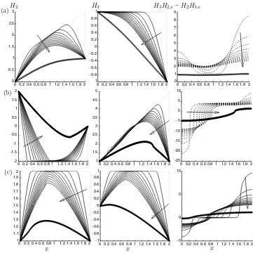
Figure 1 shows the results of three numerical calculations of the solution to (1.9)–(1.10). In Figure 1(a), the initial conditions (H2, H3) = (1 +x,1) are used and at time t = 0
the boundary magnetic fields are switched to (H2, H3)|x=0 = (0,1), (H2, H3)|x=2 = (1,−1).
In the resulting evolution, the diffusion never goes to zero and the solutions are thus non-singular. This is essentially because the end state the solution approaches for large time (H2=x/2,H3= 1−x,H3H2x−H2H3x= 1/2) has the same sign forH3H2x−H2H3x as the initial state. In contrast, in Figure 1(b), the initial conditions (H2, H3) = (−2,1 + 2x)
take a different sign for H3H2x−H2H3x than the state the solution approaches for long times (H2, H3) = (2−x,1 + 2x). Hence the solution displays a singularity at which H3H2x−H2H3x= 0. In Figure 1(c) an impulsive change is made to an initially constant magnetic field of (H2, H3) = (2,1). Initially, two free boundaries propagate in from each
boundary (most clearly seen in the plot ofH3H2x−H2H3x). These eventually meet in the middle of the sample, where they form a singularity withH3H2x−H2H3x taking different signs on either side of it. For long times (longer than is shown in the plots) all three solutions tend towards a unique steady state of the form H2 = ax+b, H3 = cx+d
satisfying the boundary data imposed on the edge of the sample. This seems to be typical behaviour for such solutions and backs up the conjecture made in (2.8).
4 A complete catalogue of similarity reductions
We apply the usual Lie group method for determining the classical point symmetries of (1.9)–(1.10) (see for example Bluman and Cole [3]), in the first instance by determining the infinitesimal transformations of the form
t∗∼t+εT(H2, H3, x, t), x∗∼x+εX(H2, H3, x, t), H2∗∼H2+εK2(H2, H3, x, t), H3∗∼H3+εK3(H2, H3, x, t),
which leave equations (1.9)–(1.10) unchanged to orderε, whereε1. Omitting the details of the derivation, we find the symmetry group of (1.9)–(1.10) has seven parameters and takes the form
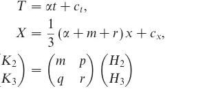
T =αt+ct, (4.1)
X= 1
3(α+m+r)x+cx, (4.2)
K2 K3
=
m p
q r
H2 H3
(4.3)
0 0.2 0.4 0.6 0.8 1 1.2 1.4 1.6 1.8 2 2 −1.5 −1 −0.5 0 0.5 1 1.5 2
0 0.2 0.4 0.6 0.8 1 1.2 1.4 1.6 1.8 2 1 1.5 2 2.5 3 3.5 4 4.5 5
0 0.2 0.4 0.6 0.8 1 1.2 1.4 1.6 1.8 2
−25 −20 −15 −10 −5 0 5 10 0 0.2 0.4 0.6 0.8 1 1.2 1.4 1.6 1.8 2
0 0.5 1 1.5 2 2.5 3
0 0.2 0.4 0.6 0.8 1 1.2 1.4 1.6 1.8 2 1 −0.8 −0.6 −0.4 −0.2 0 0.2 0.4 0.6 0.8 1
0 0.2 0.4 0.6 0.8 1 1.2 1.4 1.6 1.8 2 0 1 2 3 4 5 6 7 8 9
0 0.2 0.4 0.6 0.8 1 1.2 1.4 1.6 1.8 2
−5 0 5 10
0 0.2 0.4 0.6 0.8 1 1.2 1.4 1.6 1.8 2 1 1.1 1.2 1.3 1.4 1.5 1.6 1.7 1.8 1.9 2
0 0.2 0.4 0.6 0.8 1 1.2 1.4 1.6 1.8 2
−1 −0.8 −0.6 −0.4 −0.2 0 0.2 0.4 0.6 0.8 1 (b)
(a)H2 H3 H3H2,x H2H3,x
(c)
x x x
[image:10.493.73.434.57.417.2]–
Figure 1. (a) Evolution of magnetic fields, following an impulsive change of the boundary magnetic fields, from an initial configuration (dotted line), at uniformly spaced intervals betweent= 0.0833 and t = 0.1 (solid lines). The final curve (circles) shows the magnetic field at t = 0.5. (b) An impulsive change of magnetic field from initial configuration (H2, H3) = (−2,1 + 2x) plotted at uniform intervals betweent= 0.001667 and t= 0.02 (solid lines) the final curve (thick line) is at t= 0.1. Note that this solution displays a singularity at whichH3H2x−H3H2x= 0. (c) An impulsive change to the initially constant magnetic field (H2, H3) = (2,1). The dotted line shows the initial conditions after that plots are at uniform intervals betweent= 0.008333 and t= 0.1 (solid lines) and a final plot is made att= 0.5 (thick line). Note the presence of two free boundaries propagating in from the edge of the sample.
translations intandx;αa rescaling intandx, andm,p,q andran affine transformation inH2 andH3. In fact, the Lie Group for (H2, H3) is the affine group A(2).
by making an appropriate rotation of the (H2, H3) coordinates. The simplified catalogue
of reductions then takes the form
H2= (±t)βG(η) +K(±t)µF(η) H3= (±t)µF(η)
η=x(±t)−(µ+β+1)/3
(4.4)
H2= exp(βt)G(η) +Kexp(µt)F(η) H3= exp(µt)F(η)
η=xexp
−µ+β
3 t (4.5)
H2=K(±x)3−βF(t) + (±x)βG(t) H3= (±x)3−βF(t)
(4.6)
H2= (±t)µG(η) +K(±t)−(1+µ)F(η) H3= (±t)−(1+µ)F(η)
η=x−plog(±t)
(4.7)
H2= exp(−µt)G(η) +Kexp(µt)F(η) H3= exp(µt)F(η)
η=x−qt
(4.8)
H2 = exp(−µx)G(t) +Kexp(µx)F(t) H3 = exp(µx)F(t)
(4.9)
H2= (±t)3βρ(η) cos (Ωlog(±t) +φ(η)) +Lsin (Ωlog(±t) +φ(η)) H3=K(±t)3βρ(η) sin (Ωlog(±t) +φ(η))
η=x(±t)−(2β+1/3)
(4.10)
H2= exp
−3 2µt
ρ(η) cos (Ωt+φ(η)) +Lsin (Ωt+φ(η))
H3= exp
−3 2µt
ρ(η) sin (Ωt+φ(η))
η=xexp (µt)
(4.11)
H2= (±x)3/2ρ(t) [cos (Ωlog(±x) +φ(t)) +Lsin (Ωlog(±x) +φ(t))] H3=K(±x)3/2ρ(t) sin (Ωlog(±x) +φ(t))
(4.12)
H2= (±t)−1/2ρ(η) [cos (Ωlog(±t) +φ(η)) +Lsin (Ωlog(±t) +φ(η))] H3=K(±t)−1/2ρ(η) sin (Ωlog(±t) +φ(η))
η=x−qlog(±t)
H2=ρ(x−qt) [cos(Ωt+φ(x−qt)) +Lsin(Ωt+φ(x−qt))] H3=Kρ(x−qt) sin(Ωt+φ(x−qt))
(4.14)
H2=ρ(t) [cos(Ωx+φ(t)) +Lsin(Ωx+φ(t))] H3=Kρ(t) sin(Ωx+φ(t))
(4.15)
H2= (±t)βG(η) +K(±t)βlog(±t)F(η) H3= (±t)βF(η)
η=x(±t)−(2β+1)/3
(4.16)
H2= exp(βt) [G(η) +qtF(η)] H3= exp(βt)F(η)
η=xexp
−2 3βt
(4.17)
H2= (±x)3/2(G(t) +qlog(±x)F(t)) H3= (±x)3/2F(t)
(4.18)
H2= (±t)−1/2G(η) +q(±t)−1/2log(±t)F(η) H3= (±t)−1/2F(η)
η=x−plog(±t)
(4.19)
H2 = (±t)−1/2(G(x) +qF(x) log(±t)) H3 = (±t)−1/2F(x)
(4.20)
H2=G(η) +KtF(η) H3=F(η)
η=x−qt
(4.21)
H2=G(t) +qxF(t) H3=F(t)
(4.22)
where K, β, µ, p, q, Ω and L are all arbitrary constants. To retrieve the full similarity reductions from this list, one needs simply to make a rotation of the (H2, H3) axes of the
form
H2→cos(χ)H2−sin(χ)H3, H3→cos(χ)H3+ sin(χ)H2,
(whereχis arbitrary) so that, for instance, (4.4) now becomes
H2= cos(χ)(±t)βG(η) + (Kcos(χ)−sin(χ)) (±t)µF(η), H3= (cos(χ) +Ksin(χ)) (±t)µF(η) + sin(χ)(±t)βG(η), η=x(±t)−(µ+β+1)/3.
5 Travelling wave solutions
Where we look for travelling wave solutions to (1.9)–(1.10) of the form
H2= cos(χ)G(x−qt)−sin(χ)F(x−qt), H3= cos(χ)F(x−qt) + sin(χ)G(x−qt), η =x−qt,
(whereK andχare arbitrary constants) we obtain the following equations for F andG:
−qF= d
dη(F
|FG−GF|), (5.1)
−qG= d
dη(G
|FG−GF|). (5.2)
We also note that
H3H2x−H2H3x= (FG−GF).
Subtracting (5.1) multiplied byGfrom (5.2) multiplied byF yields the following equation: −q(FG−GF) = (FG−GF)|(FG−GF)|+ (FG−GF)|(FG−GF)|.
Assuming that (FG−GF)>0, we find
(FG−GF) =−q
2(η−η0) for (η0−η)sgn(q)>0, or (FG
−GF) = 0, (5.3)
where η0 is a constant of integration. Substituting (5.3) back into (5.1) and (5.2) we find
thatF andGtake the form
F =A+B(η−η0)2,
G=
q
4B + AC
B
+C(η−η0)2,
for (η0−η)sgn(q)>0, (5.4)
F =A and G=
q
4B+ AC
B
for (η0−η)sgn(q)<0, (5.5)
To find solutions with (FG−GF) 6 0 we replace q by −q everywhere in (5.3) and (5.4)–(5.5), except in the inequalities (η0−η)sgn(q)>0 and (η0−η)sgn(q)<0.
6 Similarity solutions describing impulsive changes from a constant magnetic field
In this section, we look for a similarity solution which describes the short-time evolution of the magnetic field when the boundary field, atx= 0 say, is changed impulsively. With this in mind we look for solutions to (1.9)–(1.10) of the form
H2 =G(η), H3 =F(η), η=xt−1/3,
ODEs forF andG
−η 3F
= d
dη(F
|FG−GF|), (6.1)
−η 3G
= d
dη(G
|FG−GF|). (6.2)
Multiplying (6.1) byGand subtracting (6.2) multiplied byFthen gives rise to the following equation for the diffusion coefficientFG−GF:
η
3(FG
−GF) + d
dη((FG
−GF)|FG−GF|) = 0,
which we can solve to find
FG−GF=±1 12(A
2−η2) for η26A2,
FG−GF= 0 for η2>A2,
(6.3)
whereA is a constant of integration. Substituting the solution for FG−GF (6.3) back into (6.1) and (6.2) and integrating forF andG, we find
H2=G=
1 12
b2−h2
|h3b2−h2b3|
A2η−η 3
3
+h2
H3=F =
1 12
b3−h3
|h3b2−h2b3|
A2η−η 3
3
+h3
for η26A2, (6.4)
H2 =G=b2, H3=F=b3, for η2>A2, (6.5)
η =xt−1/3 (6.6)
whereAis given in terms of the four constants of integrationh2, h3, b2, b3 by
A3= 18|h3b2−h2b3|. (6.7)
The similarity solution (6.4)–(6.7) satisfies the following initial value problem:
H2=b2, H3=b3, for t= 0 x>0, (6.8)
H2=h2, H3=h3, on x= 0 t >0, (6.9)
and thus describes the evolution from an initially constant field (H2, H3) = (b2, b3) in
a half-space, when the magnetic field on the boundary x = 0 is impulsively changed to (H2, H3) = (h2, h3) at timet= 0+. This similarity solution breaks down whenh3b2−h2b3=
0; this is because the change to the magnetic field (applied on the boundary) is then in the same direction as the magnetic field within the sample. Since the model is invariant under rotation, this is equivalent to setting H3 ≡0 throughout the evolution, and since
0 0.2 0.4 0.6 0.8 1 1.2 1.4 1.6 1.8 2 0
0.1 0.2 0.3 0.4 0.5 0.6 0.7 0.8 0.9 1
0 0.2 0.4 0.6 0.8 1 1.2 1.4 1.6 1.8 2 0
0.1 0.2 0.3 0.4 0.5 0.6 0.7 0.8 0.9 1
x H2
[image:15.493.59.425.58.234.2]x H3
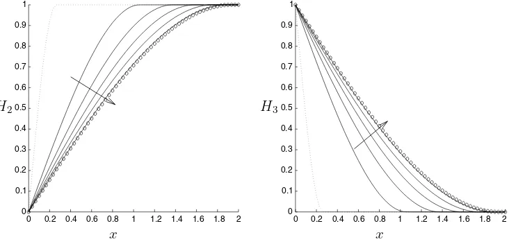
Figure 2. Comparison between numerical solution to (1.9)–(1.10) and the similarity solution (6.4)– (6.6). The numerical solution is plotted at equally spaced intervals between times t = 0.01 and t= 0.4 (dotted and solid lines). The similarity solution is shown att= 0.4 (circles).
for whichh3b−h2d= 0. This motivates the search for another type of similarity solution
in §7.
Numerical evidence suggests that the similarity solution (6.4)–(6.6) provides the short time behaviour of the solution to (1.9)–(1.10) in a slab where an initially constant magnetic field is subjected to an impulsive changes of the boundary magnetic fields. An example of this is provided in Figure 2. This figure shows a numerical solution of (1.9)–(1.10) on the finite domain 0 < x <2. Initial data for the simulation is provided by the similarity solution at t= 0.01, and the boundary data H2(0, t) = 0, H3(0, t) = 1, H2(2, t) = 1,H3(0, t) = 0 is imposed. The final plot from this simulation is att= 0.4 and
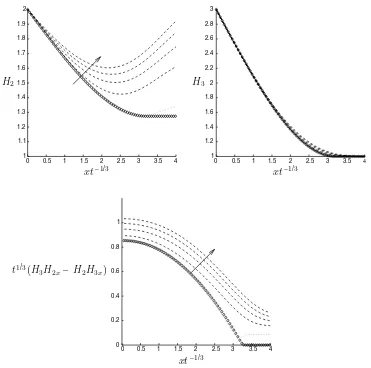
is compared to the similarity solution (6.4)–(6.6) at the same time (plotted with circles). Note that the similarity solution is exact until the free-boundary x= At1/3 reaches the far side of the slab x = 2. In addition we also might expect this similarity solution to provide the short time behaviour to the equivalent scenario with initial condition provided by the steady solution (2.1). This is exemplified by Figure 3, in which the initial magnetic field in the slab 0 < x < 2 is H2 = 1 +x/2, H3 = 1 and, at time t = 0,
the magnetic field on the left-hand boundary is impulsively changed to H2|x=0 = 2, H3|x=0= 3.
Remark 1 This type of solution also describes the evolution of two regions of uniform magnetic field in x <0 andx >0 which start to interact at time t= 0. In other words, given the initial conditions
H2=b2, H3 =b3 for x >0 H2=h2, H3 =h3 for x <0
0 0.5 1 1.5 2 2.5 3 3.5 4 1
1.1 1.2 1.3 1.4 1.5 1.6 1.7 1.8 1.9 2
0 0.5 1 1.5 2 2.5 3 3.5 4
1 1.2 1.4 1.6 1.8 2 2.2 2.4 2.6 2.8 3
0 0.5 1 1.5 2 2.5 3 3.5 4
0 0.2 0.4 0.6 0.8 1
xt−1/3
H2
xt−1/3
H3
xt−1/3
t1/3(H
[image:16.493.70.441.52.420.2]3H2x– H2H3x)
Figure 3. A numerical simulation showing the evolution from a steady solution of the form H2 =ax+b,H3 =cx+dto which an impulsive change of the boundary field att= 0 is made. The solution is plotted at equally spaced intervals between timest= 0.005 andt= 0.1 (dotted and dashed lines). The similarity solution is shown by circles.
the subsequent evolution is described by
H2=G=
(b2−h2)
12|b2h3−h2b3|
A2η−η 3
3
+1
2(b2+h2),
H3=F=
(b3−h3)
12|b2h3−h2b3|
A2η−η 3
3
+1
2(b3+h3)
for |η|< A,
where
η=xt−1/3, A3= 9|b2h3−h2b3|.
Remark 2 The similarity reductionH2 =G(η),H3=F(η),η=x(−t)−1/3is of less physical
interest because, as η → ∞the solutions to F and Gare both cubic in η (i.e. F ∼Mη3, G∼Nη3).
7 Similarity solutions describing an impulsive change to the boundary magnetic field with initial conditions H2=ax+b, H3 =cx+d
As stated in the previous section the similarity solution (6.4)–(6.6), which describes the change from a constant field H = (b2, b3,0) when a field H = (h2, h3,0) is impulsively
applied on the boundary, breaks down whenh3b2−b3h2= 0. This is because the applied
field then lies in the same direction as the initial magnetic field. In this section, we look for similarity solutions with initial profile of the form H2=ax+b,H3=cx+d to which
an impulsive change of magnetic field (H2, H3,0)|x=0 = (h2, h3,0) is applied at t= 0+ in
the same direction as the field on the boundary so thath2d−h3b= 0. To do this we look
for similarity solutions of the form (4.4) with β = 0, µ= 1/2. For simplicity, we write these in their simple forms:
H2=G
xt−1/2+Kt1/2Fxt−1/2, H3=t1/2F
xt−1/2, η =xt−1/2
(7.1)
or
H2=G
x(−t)−1/2+K(−t)1/2Fx(−t)−1/2, H3= (−t)1/2F
x(−t)−1/2, η=x(−t)−1/2,
(7.2)
and recall that we can apply an arbitrary rotation of the (H2, H3)-plane to obtain the
more general form.
7.1 Similarity solutions with the form (7.1)
Substituting (7.1) into (1.9)–(1.10) gives rise to the following equations forF andG:
1 2F−
η
2F
= d
dη(F
|FG−GF|), (7.3)
−η 2G
= d
dη(G
|FG−GF|), (7.4)
which are invariant under three separate discrete transformations
(i)η→ −η, (ii)F → −F, (iii)G→ −G. (7.5)
We note that
and hence that whereverFG−GF vanishes the diffusion coefficient in (1.9)–(1.10) also does so. This system also exhibits two Lie point symmetries and so we could reduce it to a second order non-autonomous system; however we obtain no significant advantage from doing so, and hence choose instead to solve the full system numerically.
Motivated by the initial value problem
H2 =m+nx, H2=kx, for t= 0, H2|x=0=β, H3|x=0= 0, for t >0,
(7.6)
we look for solutions to (7.3)–(7.4) satisfying the boundary conditions
F =O(η), G∼β as η→0,
F∼kη, G∼m as η → ∞. (7.7)
HereK=n/k. Assuming that we can find solutions to this boundary value problem, then the long time behaviour of the corresponding solutions toH2 andH3 is given by
H2∼β+Kαx H3∼kx
as t→ ∞,
whereα is a constant determined by the smallη behaviour of the solution for F in the following manner:
F∼αη, G∼β+O(η) asη→0. (7.8)
It is notable that the smallη behaviour is non-singular, and so exhibits three degrees of freedom.
7.1.1 Asymptotic behaviour of solutions as η→ ±∞
We now look for possible asymptotic behaviours of solutions to (7.3)–(7.4) for large η. We start by noting that only one exact polynomial solution exists to this system; that is
F =kη, G=m, (7.9)
wherekandmare arbitrary constants. In addition to being an exact solution of (7.3)–(7.4) it is possible for other solutions of this system to asymptote to it asη→ ±∞.
To calculate the number of degrees of freedom exhibited by solutions asymptoting to (7.9), we shall assume that km <0, so that FG−GF > 0, and perturb about (7.9) as follows:
F∼kη+F1, G∼m+G1, η → ±∞,
system which we solve to obtain the four eigenmodes
F1=η G1= 0
; F1∼ 1
η2exp
− η2 8|km|
G1= 0
;
F1= 0 G1= 1
;
F1 ∼ − k mexp
− η2 4|km|
G1 ∼
1
η exp
− η2 4|km|
.
The first and third of these correspond to a small change in k and m, respectively, and the second and fourth are both compatible with the asymptotic behaviour (7.9); it follows that this asymptotic behaviour has four degrees of freedom and is thus generic. By the symmetry of the system the same result clearly holds forkm >0.
Given that this behaviour exhibits four degrees of freedom and the behaviour atη= 0 exhibits three degrees of freedom we might expect that the boundary value problem comprising equations (7.3)–(7.4) and boundary conditions (7.7) to be well-posed.
7.1.2 Finiteη blow-up of solutions to(7.3)–(7.4)
The system (7.3)–(7.4) exhibits singular behaviour only asη→ ±∞or asFG−GF→0. The latter leads to solutions with finiteηblow-up. We have identified two broad classes of such behaviour and believe these to be the only ones. In order to simplify the presentation we write down one example of each class of behaviour noting that we can generate the rest of the class (seven more examples) by application of different combinations of the transformations found in (7.5).
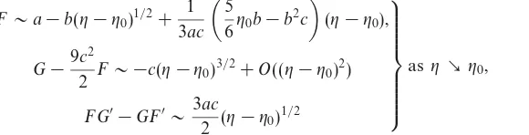
An example of the first class of behaviour is
F∼a+b(η0−η)1/2+
1 3ac
5 6η0b−b
2c
(η0−η),
G−9c 2
2 F ∼ −c(η0−η)
3/2+O((η 0−η)2)
FG−GF∼ 3ac
2 (η0−η)
1/2
asηη0, (7.10)
where b and η0 are arbitrary constants a >0 and c > 0. Since there are four constants
over which we have choice the behaviour is generic (i.e.has four degrees of freedom). An example of the second class of behaviour is
F∼a
1− 2
η0
(η0−η)−
3 2η02
(η0−η)2log|η0−η|
G∼ −η0
8a(η0−η) 2− 1
48a(η0−η) 3
FG−GF∼ η0
4(η0−η)
wherea >0 andη0 >0 but are otherwise arbitrary. We assess the number of degrees of
freedom exhibited by this behaviour by perturbing about it as follows:
F∼a
1− 2
η0
(η0−η)−
3 2η0
(η0−η)2log(η0−η)
+F1,
G∼ −η0
8a(η0−η) 2− 1
48a(η0−η) 3+G
1
as ηη0,
substituting into (7.1), linearising inF1 andG1and seeking eigenmodes to obtain a fourth
order linear homogeneous system. The solution to this system, at leading order in (η0−η),
gives the eigenmodes
F1 ∼1−
2
η0
(η0−η)
G1 ∼ η0
8a2(η0−η) 2 ;
F1∼ −
2a η0 G1∼ −
η0
4a(η0−η)
;
F1∼(η0−η)2 G1∼O((η0−η)4)
;
F1∼ −
4a2 η3
0
log(η0−η)
G1∼1−
1
η0
(η0−η) log(η0−η)
.
The first two of these correspond to small changes in a and η0 respectively; the third
is compatible with asymptotic behaviour (7.11) while the fourth is not (F1 being much
larger thanF in (7.11)). Asymptotic behaviour (7.11) can thus be seen to exhibit three degrees of freedom.
7.1.3 Solutions with compact support in the diffusion coefficient |H3H2x−H2H3x|=|FG−GF|, and singular solutions
We can form solutions to (7.3)–(7.4) with compact support in |FG−GF| by taking a half solution with behaviour (7.11) asηη0 (withη0 >0) and continuing it by the half
solution
F=−kη, G= 0, FG−GF= 0, η > η0 (7.12)
atη=η0. At the join we must ensure continuity ofF andG,
[F]η=η0= 0, [G]η=η0 = 0,
but sinceFG−GF = 0 at the point η =η0 there is no requirement on the continuity
of F and G. However, we also require continuity of the flux of the fields (H2,H3); this
enforces the condition
F(FG−GF)→0 and G(FG−GF)→0 asη→η0.
Applying these conditions we see that
k=−a
We can also form continuous singular solutions to (7.3)–(7.4) by joining the half solution with behaviour (7.10) as ηη0 to the half solution with behaviour
F∼a−b(η−η0)1/2+
1 3ac
5 6η0b−b
2c
(η−η0),
G−9c 2
2 F ∼ −c(η−η0)
3/2+O((η−η 0)2)
FG−GF∼ 3ac
2 (η−η0)
1/2
asηη0, (7.13)
(this behaviour is another member of the class of behaviours to which (7.10) belongs). This ensures that at the pointη=η0there is continuity ofF andG, and furthermore that
the jump conditions
[F(FG−GF)]η=η0= 0, [G(FG−GF)]η=η0= 0,
are satisfied and hence that there is continuity in the flux ofH2 andH3.
Remark We can form other solutions with compact support in |H3H2x−H2H3x|, and other singular solutions, by applying any combination of the discrete transformations (7.5) to the solutions we obtain using the methods outlined above.
7.1.4 Numerical solution of equations (7.3)–(7.4)
We used a fourth order Runge-Kutta scheme to solve equations (7.3)–(7.4). We found (i) regular solutions, (ii) solutions with compact support in the diffusion coefficientFG−GF
and (iii) solutions with an internal singularity. In all cases we required the solution behave like (7.8) at the origin. When searching for solutions to equations (7.3)–(7.4) it is helpful to bear in mind that these equations are invariant under a two parameter group of rescalings
F→mF, G→ ±|q| 3
|m|G, η→qη. (7.14)
We can use this rescaling invariance to reduce the amount of work needed in searching the solution space. So for example when we look for a solution of the form (i), imposing the condition (7.8) at the origin, it appears that we should obtain a three-parameter family of solutions. However once we have taken account of the invariance of the system to rescalings of the form (7.14) we see that this in fact only a one parameter family of solutions; the other two degrees of freedom merely represent rescalings. Similarly, solutions of the form (ii) have a zero-parameter family of solutions once rescaling have been taken into account and solutions of the form (iii) have a one-parameter family of solutions once rescalings have been accounted for.
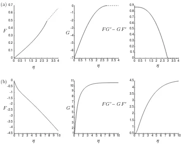
An example of (i) which asymptotes to (7.9) as η → ∞ is given in Figure 4(b). An example of (ii) which has behaviour (7.11) as ηη0= 3 and, for η >3, has form (7.12)
[image:21.493.107.397.91.165.2]0 0.5 1 1.5 2 2.5 3 3.5 4 0 0.1 0.2 0.3 0.4 0.5 0.6 0.7
0 0.5 1 1.5 2 2.5 3 3.5 4
−7 −6 −5 −4 −3 −2 −1 0
0 0.5 1 1.5 2 2.5 3 3.5 4 0 0.1 0.2 0.3 0.4 0.5 0.6 0.7 0.8 0.9
0 1 2 3 4 5 6 7 8 9 10
−4.5 −4 −3.5 −3 −2.5 −2 −1.5 −1 −0.5 0
0 1 2 3 4 5 6 7 8 9 10 1 2 3 4 5 6 7 8 9 10 11
0 1 2 3 4 5 6 7 8 9 10 0.5 1 1.5 2 2.5 3 3.5 4 4.5 F G G
F F G′ − G F′
[image:22.493.72.435.52.343.2](a) (b) η η η η η η F G′ − G F′
Figure 4. Two examples of similarity solution of the form (7.1) with the behaviour (7.8) asη→0. In (a) we give an example of a solution with compact support which has asymptotic behaviour (7.11) at the pointη=η0= 3 and which is extended beyond this point by a solution of form (7.12) (the dashed line). In (b) the solution asymptotes to a solution of the form (7.9) asη→ ∞.
0 1 2 3 4 5 6
0 1 2 3 4 5 6 7 8 9
0 1 2 3 4 5 6 0 1 2 3 4 5 6
−5 0 5 10 15 20 25 30 −20 −15 −10 −5 0 5 F G
η η η
F G′ − G F′
[image:22.493.81.432.442.579.2]0 0.5 1 1.5 2 2.5 3 3.5 4 0
0.1 0.2 0.3 0.4 0.5 0.6 0.7 0.8 0.9
0 0.5 1 1.5 2 2.5 3 3.5 4 0
0.1 0.2 0.3 0.4 0.5 0.6 0.7
0 0.5 1 1.5 2 2.5 3 3.5 4
−7
−6
−5
−4
−3
−2
−1 0
0 0.2 0.4 0.6 0.8 1 1.2 1.4 1.6 1.8 2
−2
−1.5
−1
−0.5 0 0.5 1 1.5 2 2.5 3 3.5
0 0.2 0.4 0.6 0.8 1 1.2 1.4 1.6 1.8 2 0
0.2 0.4 0.6 0.8 1 1.2 1.4 1.6 1.8 2
0 0.2 0.4 0.6 0.8 1 1.2 1.4 1.6 1.8 2
−3
−2.5
−2
−1.5
−1
−0.5 0 0.5 1 1.5
H3H2x−H2H3x H2 t−1/2H3
xt−1/2
xt−1/2
H2 H3 H3H2x H2H3x
xt−1/2
x x x
(b) (a)
[image:23.493.57.421.58.342.2]−
Figure 6. Comparison of numerical solutions to the PDEs with corresponding similarity solution. (a) Comparison to a similarity solution with a free boundary (see Figure 4a):-dashed lines show the numerical solutions plotted at evenly spaced intervals up to t = 0.5 while circles show the similarity solution att= 0.5. (b) Comparison to a similarity solution with a singularity:- solid lines show numerical solution plotted at evenly spaced intervals up tot= 0.15, dotted line show initial condition, and crosses show the similarity solution at t = 0.15. In both cases the computational domain is 06x63.
solution and a solution to the the partial differential equations (1.9)–(1.10) is made in Figure 6.
Numerical work shows that regular solutions (i) to (7.3)–(7.4) which asymptote to (7.8) asη0 and are linear at infinity (7.9) and have the same sign ofFG−GFthroughout. In contrast to this, singular solutions (iii) to (7.3)–(7.4), which asymptote to (7.8) asη 0 and are linear at infinity and have FG−GF which changes sign between the origin and infinity.
7.1.5 Solutions to (7.3)–(7.4)for whichGis a constant
Solutions to (7.3)–(7.4) exist for whichGis constant. Assuming that FG−GF>0 and writing
leads to the following second order ODE forF:
dF dη
4νd 2F dη2 +η
−F= 0, νdF
dη >0. (7.16)
We consider only the case ν > 0, since this equation is invariant under the discrete transformation
ν→ −ν, F→ −F.
We could now, by rescaling F and η, scaleν out of (7.16). We thus need only consider one value ofν. We use the fact that this equation is invariant under the transformation
F→k3F, η→kη,
to write (7.16) in autonomous form by introducing new variables ζ and y (an invariant of this transformation) defined by the relations
y= F
η3, ζ= log|η|. (7.17)
Since (7.16) is invariant under the discrete transformation
F → −F, η → −η,
we restrict our attention to solutions for whichη >0. Application of (7.17) to (7.16) then yields the following second order autonomous system
dy dζ =z, dz dζ =−
1 4ν
z+ 2y z+ 3y
−5z−6y
whereν(z+ 3y)>0 andη >0. (7.18)
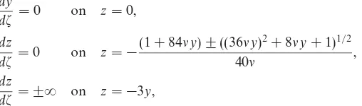
We can describe the nature of solutions to (7.18), and hence to (7.16) also, by sketching the associated phase plane. The null clines of this system are given by
dy
dζ = 0 on z= 0, dz
dζ = 0 on z=−
(1 + 84νy)±((36νy)2+ 8νy+ 1)1/2
40ν ,
dz
dζ =±∞ on z=−3y,
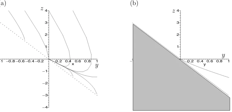
In the region of interest there is a singular point at the origin and no critical points. In Figure 7(b) the null clines of (7.18) are plotted, together with the singular liney+ 3z= 0, for a typical case. The corresponding phase plane is plotted in Figure 7(a).
Asymptotic behaviours of the phase trajectories
Asζ→ −∞(7.18) the solutions to (7.18) exhibit the following behaviour:
y∼Aexp(−3ζ) +Bexp(−2ζ) + A
[image:24.493.127.381.436.511.2]−4
−3
−2
−1 1 2 3 4
−1 −0.8−0.6−0.4−0.2 0.2 0.4 0.6 0.8 1 x
ñ4 ñ3 ñ2 ñ1 1 2 3 4
−1 ñ0.8 ñ0.6 ñ0.4 ñ0.2 0.2 0.4 0.6 0.8 1 y
z
z
y
y
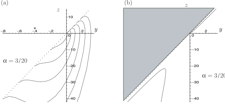
[image:25.493.51.434.57.243.2](a)
(b)
Figure 7. (a) Typical phase paths for the system (7.18) (in this caseν= 1/20); (b) typical null-clines (dotted lines) and line of singularity (solid line) for the system (the forbidden region of the phase plane is shaded).
where Aand B arbitrary; thus z∼ −3y as y → ∞ and the corresponding behaviour for
F is
F∼A+Bη η0. (B >0) (7.19)
As the phase trajectories approach the linez+ 3y= 0 they exhibit either the behaviour
y∼y0−3y0(ζ−ζ0) +
1 3
2y0 ν
1/2
(ζ−ζ0)3/2 fory0>0,
or the behaviour
y∼y0+ 3y0(ζ0−ζ)−
1 3
−2y0 ν
1/2
(ζ0−ζ)3/2 fory0 <0.
The corresponding behaviours for F are
F ∼y0η03+
1 3
2y0η30 ν
1/2
(η−η0)3/2 asη η0 (y0>0, η0>0), (7.20)
and
F ∼y0η30−
1 3
−2y0η30 ν
1/2
(η0−η)3/2 asηη0 (y0 <0, η0>0), (7.21)
respectively. The latter is equivalent to (7.10) withb= 0 while the former is equivalent to (7.10) with b= 0 where we make the transformation η → −η and G→ −G. Finally, we note that trajectories which approach the origin have asymptotic behaviour of the form
and the corresponding behaviour forF is
F∼Aη η→ ∞. (7.22)
The phase plane reveals that we can find solutions to (7.16) (with positiveν) which link the asymptotic behaviours (7.19) (with A < 0) to (7.21); (7.19) (with A > 0) to (7.22); and (7.20) to (7.22). The only solution to (7.16), which behaves like (7.8) at the origin is the explicit solutionF =Bη (which corresponds to the straight-line solutionz=−2y of (7.18)). It is clear that no solutions exist with compact support inFG−GF (=νF) and that although we can form singular solutions, as in §7.1.3, that these solutions do not exhibit behaviour (7.8) at the origin. The solutions we can find to (7.16) are thus of little physical interest.
7.1.6 Summary
The phase plane analysis we have conducted above reveals that the only solutions to (7.3)–(7.4) withG=const. which exhibit local behaviourF ∼αηas η→0 take the form
F =αη. Relaxing the constraint on G, and allowing it to be non constant, allows us to find families of solutions to (7.3)–(7.4) which exhibit the behaviour
F∼αη, G∼β+pη, as η →0 and which asymptote to a linear solution for largeη
F∼kη, G∼m asη → ±∞.
The preceding analysis suggests that, when solving forF and G, we should specify three of the five parameters (α, β, p, k, m). The motivating initial value problem (7.6) suggests we specify (β, k, m). Assuming that we solve only in η > 0 such solutions can either be (i) regular; (ii) have compact support in the diffusion coefficient FG−GF and a corresponding free boundary; or (iii) have an internal singularity. Examples of such solutions are plotted in Figures 4(b), 4(a) and 5 respectively. In Figure 6 comparison is made between numerical solutions calculated from appropriate initial data and two members of this class of similarity solution. Physically such solutions describe the evolution from a steady solution of the form (2.1) in a half-space when an impulsive change of the magnetic field is made on the boundaryx= 0. The evolution is towards another steady solution of the form (2.1). More details on the physical interpretation of such solutions are provided in the conclusion to this work.
7.2 Similarity solutions with the form (7.2)
Substituting (7.2) into (1.9)–(1.10) gives the following equations forF andG:
−
1 2F−
η
2F
= d
dη(F
|FG−GF|), (7.23)
η
2G = d
dη(G
|FG−GF|). (7.24)
We also note that, in this instance,