Department of Economics University of Southampton Southampton SO17 1BJ UK
Discussion Papers in
Economics and Econometrics
OMITTED VARIABLES IN COINTEGRATION ANALYSIS
Nicoletta Pashourtidou No. 0304
This paper is available on our website
ISSN 0966-4246
DISCUSSION PAPERS
IN ECONOMICS AND ECONOMETRICS
OMITTED VARIABLES IN COINTEGRATION ANALYSIS
Nicoletta Pashourtidou1
School of Economic Studies, University of Manchester, Manchester M13 9PL
Discussion Paper 0304
June 2003
Abstract: This paper investigates the effects of the omission of relevant variables
from the statistical model on cointegration analysis, proposed by Johansen (1988,
1991). We show that underspecification of the statistical model leads to either failure
in detecting cointegration or underestimation of the cointegrating rank. Although in
the underspecified statistical model the estimator of the detected cointegrating vectors
is shown to be consistent, this is not the case for the estimators of the adjustment
coefficient matrix and the variance of the error term. The asymptotic analysis is
supplemented by a Monte Carlo experiment and an empirical example.
Key words: cointegration, omitted variables, asymptotics, Monte Carlo
JEL: C15, C32, C52
1I am greatly indebted to Raymond O’Brien who motivated and supervised this paper. Comments
I. Introduction
The likelihood ratio (LR) tests for cointegration proposed by Johansen (1988, 1991)
have been widely applied in empirical research and it is of interest to study their
behaviour under various types of misspecification of the statistical model (SM) used
for cointegration testing. The robustness of the LR tests for cointegration has been
investigated using Monte Carlo simulations under omitted or irrelevant (redundant)
step and impulse dummy variables (see Andrade et al., 1994), dynamic
misspecifica-tion using a data generating process (DGP) with autoregressive and moving average
dynamics (see Boswijk and Franses, 1992; Cheung and Lai, 1993) and non-normality
assuming non-symmetric and leptokurtic innovations (see Cheung and Lai, 1993).
An interesting form of misspecification is the underspecification or
overspecifica-tion of the statistical model used for cointegraoverspecifica-tion testing. This means that with
respect to the DGP, either some variables have been omitted from the SM or some
of the variables included in the SM are irrelevant. Podivinsky (1998) investigates
the performance of the LR tests for cointegration (mainly the trace statistic) when
there is a mismatch between the variables used in the SM (used for the cointegration
tests) and the variables entering the true cointegrating vectors. Using Monte Carlo
simulations he finds that the LR tests performed on an overspecified SM detect at
least the true number of cointegrating vectors. He also finds that LR tests based
vectors among three variables, and (ii) may not detect a cointegrating vector if there
is only one cointegrating vector among three variables. The potential importance of
these results for the applied work is illustrated by DeLoach (2001) who uses LR tests
for cointegration (trace and maximal eigenvalue statistics) to test the hypothesis of
cointegration between the relative price of nontradables and real output (which is
consistent with the productivity-bias hypothesis of Balassa and Samuelson). In a
two variable model (relative price of nontradables, real output) he finds evidence of
cointegration for only two out of the nine countries considered. He attributes the lack
of evidence of cointegration to the fact that certain variables, which mirror long-run
determinants of the relative prices, have been omitted from the SM. After having
aug-mented the system with the variable for oil prices, he finds evidence of cointegration
for four out the nine countries.
The purpose of this study is to investigate analytically the effects of I(1)omitted
variables from the SM, on the inference about the cointegrating rank, carried out using
the LR test statistics (trace and maximal eigenvalue), proposed by Johansen (1988,
1991). The consistency of the estimators of the parameters of the error correction
model under the above form of misspecification is also considered. The analytical
findings are supplemented by a Monte Carlo investigation and an empirical example.
The literature concerning the effects of misspecifications on the LR tests for
is to provide an analytical (asymptotic) investigation of the robustness of LR tests
for cointegration when relevant variables are omitted from the SM, and therefore an
analytical formulation of earlier Monte Carlo studies.
The organisation of the paper is as follows. Section II describes the model.
Sec-tions III and IV provide some asymptotic results concerning the implicaSec-tions of
omit-ted variables for the inference about the cointegrating rank and the consistency of
the maximum likelihood estimators of the parameters of the error correction model.
Section V provides illustrations in the form of Monte Carlo simulations and an
em-pirical example. Section VI concludes. The proofs of all propositions are presented
in the Appendix.
A word on notation. The symbols ‘→p ’ and ‘→d’ denote convergence in probability
and convergence in distribution respectively, as the sample size, T, tends to infinity.
∆is thefirst difference operator,|M| denotes the determinant of a square matrixM,
sp(M) denotes the space spanned by the columns of the matrix M and In denotes
the identity matrix of dimension n. Moreover E(·), V ar(·) and plim(·) denote the
expected value, variance and probability limit of the random argument respectively.
II. The model
The DGP is given by a VAR(1) model in error correction form,
whereεt∼i.i.d.(0,Ω) andXt is a p×1, I(1)process. In addition Xt is cointegrated
so thatΠ=αβ0 (α andβ arep×r matrices) withr≤p−1 cointegrating vectorsβ
such that β0Xt∼I(0).
The SM used for cointegration testing is assumed to be underspecified i.e. it
includes only a subset of the variables in the DGP. More specifically, letH =
Ip∗
0 k×p∗
be a selection matrix, then the SM includes p∗ < pvariables given by Xt∗ =H
0
Xt so
that k ≡(p−p∗) relevant variables are omitted.
The misspecified SM takes the form of a multivariate regression ofH0∆Xt =∆Xt∗
on H0Xt−1. The relation between ∆Xt∗ and Xt∗−1 does not have an error correction
form as the model
∆Xt∗ =Π∗Xt∗−1+e∗t, t = 1,2, . . . , T (2)
is misspecified. In particular e∗
t is in general correlated with Xt∗−1. We also define
β(1) =H0β, and α(1) =H0α, but Π∗ 6=α(1)β(1)0
andΠ∗ 6=H0ΠH as HH0 6=Ip.
Althoughβ0XtisI(0),β(1)
0
X∗
t is not necessarilyI(0)since a linear combination of
I(1)variables is in generalI(1). The nature ofβ(1)0Xt∗ is determined by the variables
entering the cointegrating relations in the DGP. Since only the space spanned by the
columns of β can be estimated, in general, (r−k) cointegrating vectors (stationary
be transformed so that
β0 =
β11 β21 · · · βp1
β12 β22 · · · βp2
..
. ... ...
β1r β2r · · · βpr
≈
β+11 β +
21 · · · β +
(p−r)1 1 0 0 · · · 0 0
β+12 β+22 · · · · · · β+(p−(r−1))2 1 0 · · · 0 0
..
. ... ... ... ... ... ... ... ... ...
β+1r β
+
2r · · · β
+
(p−1)r 1
(3)
where the symbol≈denotes the row equivalent matrix ofβ0 given by (3) andp−(r−
i) =p∗−(r−k) +i,i= 1,2, . . . , r is the number of non-zero elements in thei-th row.
Given that only p∗ variables are included in the SM, we should be able to recover i
cointegrating relations (using the underspecified SM), as long as p∗−(r−k) +i≤p∗.
Thus, at most ,(r−k)(for i=r−k) cointegrating relations can be estimated from
the SM, by applying the same row operations on β(1)0 as on β0.
In what follows the analysis is based on the fact that the cointegrating vectors,
β, (as well as the adjustment coefficients, α) are not identified so β (and therefore
α) can be replaced by a non-singular transformation e.g. we can replace β0 by a
row equivalent matrix of β0. To avoid complicating the notation we retain the same
Below we distinguish two cases:
Case (i). (r−k) ≤ 0, where all the cointegrating relations in the DGP involve at
least one of the omitted variables, thereforeβ(1)0Xt∗ ∼I(1).
Case (ii). (r−k) > 0, where there are q < r, q ≥ (r−k), cointegrating relations
in the DGP which do not involve any of the k omitted variables, accounting also
for the event of fortuitous zeros. Therefore, some elements of β(1)0X∗ t, β
0
11Xt∗, say
are stationary, where β11 is a submatrix of β(1) in the following partition, β(1) = "
β11
p∗×q
β12
p∗×(r−q)
#
. Then β(1)0Xt∗ =
β011X∗ t
β012Xt∗
and β
0
11Xt∗ ∼ I(0) while β
0
12Xt∗ ∼
I(1). Here we assume that the actual cointegrating vectors can be found as thefirst
q rows of β(1)0. Nevertheless, if the above ordering is not satisfied, the cointegrating
vectors can be isolated in the first q rows of β(1)0 using elementary row operations
(see above).
The eigenvalue equation that corresponds to (2) is
|ζS11∗ −S10∗ S00∗−1S01∗ |= 0 (4)
where S∗
11 = T−1
T P t=1
(X∗
t−1 −X¯∗)(Xt∗−1 −X¯∗)
0
, S∗
00 = T−1
T P t=1
(∆X∗
t −∆¯X∗)(∆Xt∗ − ¯
∆X∗)0, S10∗ = S∗
0
01 = T−1
T P t=1
(Xt∗−1 − X¯∗)(∆Xt∗ − ∆¯X∗)
0
, X¯∗ = T−1
T P t=1
Xt∗−1 and
¯
∆X∗ =T−1PT
t=1
∆X∗ t.
The eigenvalue equation that corresponds to the DGP is
with Sij,i, j = 0,1, defined similarly in terms of the processXt (the DGP).
Note that we can partition the stochastic vector Xt into Xt =
X∗ t p∗×1
Xt(k) k×1
where
the upper(p∗×1)block holds the variables included in the SM and the lower(k×1)
block corresponds to the omitted variables. Then, S∗
ij, i, j = 0,1, is given by the top
left submatrix of the correspondingSij,i, j = 0,1.
The matrix S11∗−1S10∗ S∗− 1
00 S01∗ has the same eigenvalues as the roots of (4), which
coincide with the non-zero eigenvalues of
S∗ = (DS11D)+(DS10D)(DS00D)+(DS01D)
where D =
Ip∗ 0
p∗×k
0
k×p∗ k×0k
and here the superscript + denotes the Moore-Penrose
(generalised) inverse.
Let Q=
S∗
11 0
0 Ik
, |Q| 6= 0 then,
|ζIp−S∗|=|Q−1||Q(ζIp−S∗)|=|Q−1||S∗(ζ)|= 0,
where S∗(ζ) =Q(ζIp −S∗). Expanding the above equation,
|S∗(ζ)|= ¯ ¯ ¯ ¯ ¯ ¯ ¯ ¯
ζS∗
11−S10∗ S∗− 1
00 S01∗ 0
0 ζIk ¯ ¯ ¯ ¯ ¯ ¯ ¯ ¯
=|ζIk||ζS∗11−S10∗ S∗− 1
00 S01∗ |= 0. (5)
As expected, there arek zero eigenvalues which correspond to the omitted variables.
SM. If the LR tests are to indicate the existence of cointegration in the underspecified
model, the second factor of (5) must give some eigenvalues with positive probability
limits.
III. Inference about the cointegrating rank
In order to investigate how the inference about the cointegrating rank is affected
we need to consider the asymptotic behaviour of S∗(ζ). In particular we examine
the limiting behaviour of the eigenvalue equation corresponding to the SM, in the
stationary and non-stationary directions as defined by the DGP.
Define BT = (β, T−1/2β¯⊥), where β¯⊥ =β⊥(β
0
⊥β⊥)−1, β⊥ is p×(p−r) such that
β0β⊥= 0 and β = β(1)
p∗×r
β(2)
k×r
,β¯⊥ = ¯
β(1)⊥
p∗×(p−r)
¯
β(2)⊥
k×(p−r)
then,
|BT0 S∗(ζ)BT|= ¯ ¯ ¯ ¯ ¯ ¯ ¯ ¯
β0S∗(ζ)β T−1/2β0S∗(ζ)¯β⊥
T−1/2β¯0⊥S∗(ζ)β T−1β¯0⊥S∗(ζ)¯β⊥
¯ ¯ ¯ ¯ ¯ ¯ ¯ ¯ = ¯ ¯ ¯ ¯ ¯ ¯ ¯ ¯
ζ(β(1)0S11∗ β (1)
+β(2)0β(2)) T−1/2ζ(β(1)0S11∗ β¯ (1)
⊥ +β
(2)0¯
β(2)⊥ )
T−1/2ζ(¯β(1)0
⊥ S11∗ β (1)
+ ¯β(2)⊥ 0β(2)) T−1ζ(¯β(1)0
⊥ S11∗ β¯ (1)
⊥ + ¯β
(2)0
⊥ β¯
(2) ⊥ ) −
β(1)0S10∗ S∗− 1 00 S01∗ β
(1)
T−1/2β(1)0S10∗ S∗− 1 00 S01∗ β¯
(1)
⊥
T−1/2β¯(1)0
⊥ S10∗ S00∗−1S∗01β (1)
T−1β¯(1)0
⊥ S10∗ S00∗−1S01∗ β¯ (1) ⊥ ¯ ¯ ¯ ¯ ¯ ¯ ¯ ¯
= 0. (6)
Represen-tation Theorem which gives the following represenRepresen-tation for Xt in (1)
Xt=C t X
i=1
εi+C1(L)εt (7)
(see Johansen, 1996, Theorem 4.2). Then for the p∗-dimensional vector of variables
X∗
t included in the SM we have the following representation, by using (7),
Xt∗ =C∗ t X
i=1
εi+C1∗(L)εt (8)
where C∗ = H0
C, C∗
1(L) = H
0
C1(L) both of dimensions p∗ ×p and rank(C∗) =
min(p∗, p∗−(r−k)). Thus, for case (i)rank(C∗) =p∗ and for case (ii) rank(C∗) =
(p∗−q).
Proposition 1 gives the asymptotic results for the two cases.
Proposition 1. Case (i). When (r−k)≤ 0, let ΥT =
T−1/2Ir 0
0 Ip−r , then
|Υ0TB
0
TS∗(ζ)BTΥT| d
→|ζB∗0C∗
Z 1
0
˜
WW˜0C∗0B∗du|= 0 (9)
where B∗ = ·
β(1) β¯(1)⊥
¸
, p∗×p and W˜ =W(u)−R1
0 W(u)du with W(u) being a
p-dimensional Brownian motion with variance Ω and u∈[0,1].
Case (ii). When (r−k)>0, let ΥT =
Iq 0 0
0 T−1/2I
r−q 0
0 0 Ip−r
, then
|Υ0TBT0 S∗(ζ)BTΥT| d
|ζΣ∗β11β11−Σ
∗
β110Σ
∗−1
00 Σ∗0β11||ζB
∗0
C∗
Z 1
0
˜
WW˜0duC∗0B∗|= 0 (10)
where B∗ = ·
β12 β¯ (1)
⊥ ¸
, p∗ ×(p−q), V ar
∆X∗ t
β011Xt∗ ≡
Σ∗
00 Σ∗0β11
Σ∗β
110 Σ
∗
β11β11
and
˜
W is defined as in case (i).
(9) shows that in the limit there areproots at zerokof which exist by construction,
since the stochastic matrix B∗0C∗R01W˜W˜0C∗0B∗ has rank p∗ almost surely. This
suggests that performing the LR tests for cointegration using the underspecified model
will lead to the rejection of the hypothesis of cointegration (i.e. acceptance ofr = 0)
as the sample size becomes larger. The limit in (9) refers to case (i) where it is
assumed that all the cointegrating relations in the DGP involve at least one of the
omitted variables. Thus, all linear combinations of variables in the SM are I(1) and
therefore no cointegrating relations can be found.
(10) indicates that there are q non-zero and (p−q) zero roots in the limit, which
suggests that q cointegrating vectors can be detected in the underspecified model
as the sample size becomes large. The first factor in (10) gives the q positive roots
and the second the (p−r) zero roots. This is because in (10) the stochastic matrix
B∗0
C∗R1
0 W˜W˜
0
duC∗0
B∗with dimensions(p−q)×(p−q)has rank(p∗−q)almost surely
and the k ≡(p−p∗) zero roots appear in the second factor of (10) by construction.
The limit in (10) refers to case (ii) whereq of the cointegrating relations in the DGP
variables in the SM areI(0)and therefore some cointegrating relations can be found.
IV. Consistency
The analysis of consistency is carried out only for case (ii) where some cointegrating
vectors can be detected. For case (i) all the estimated eigenvalues converge in
prob-ability to zero and therefore the cointegrating space is consistently estimated by the
null space.
For the analysis of consistency we use the partition of β that appears in Section
II,
β =
β11
p∗×q
β12
p∗×(r−q)
β21
k×q
β22
k×(r−q)
where β21 = 0. We define B = "
β11
p∗×q
¯
β11⊥
p∗×(p∗−q)
#
and B−1 =
¯
β011
q×p∗
β011⊥
(p∗−q)×p∗
where
¯
β11⊥=β11⊥(β
0
11⊥β11⊥)−1,β¯11 =β11(β
0
11β11)−1 andβ
0
11β11⊥= 0. B andB−1 are such
that the following relationship holds
B−1B =BB−1 =β11β¯110 + ¯β11⊥β011⊥ =Ip∗. (11)
We have shown in Section III that the tests detectqcointegrating vectors, hence under
Π∗ = α
11β
0
11, where α112 and β11 arep∗ ×q matrices of rank q. The SM then takes
the form
∆Xt∗ =α11β
0
11Xt∗−1+e∗t (12)
with V ar(e∗
t)≡Λ∗.
Let βˆ11, αˆ11 and Λˆ∗ be the maximum likelihood estimators of β11, α11 and Λ∗
calculated from the SM (2) (using (4)). The parameters β11 and α11 correspond to
thep∗×q submatrices of β, α in the DGP.
For the analysis of consistency we use a linear transformation of the columns of
ˆ
β11, which also maximises the likelihood function3 given by
˜
β11 = ˆβ11(¯β
0
11βˆ11)−1 (13)
= β11+ ¯β11⊥β
0
11⊥βˆ11(¯β
0
11βˆ11)− 1
= β11+ ¯β11⊥b1
where the second equality follows by using (11) andb1 =β
0
11⊥β˜11.
2Partitioning α similarly to β we obtain α =
α11
p∗×q p∗×α(12r−q)
α21
k×q
α22
k×(r−q)
, where H
0
α = α(1) =
"
α11
p∗×q p∗×α(12r−q) #
and α11 are the adjustment coefficients that correspond to the cointegrating
vectors which can be detected in the underspecified model. 3In fact for any normalisationcwe can define βˆ
c = ˆβ(c
0ˆ
β)−1 = ˜β(c0˜
β)−1; expanding around β
and normalisingβandβˆbyc0β=c0βˆ=Ir, we obtainβˆ−β= (Ip−βc
0
)(˜β−β) +Op(|β˜−β|2)(see
We also defineα˜11= ˆα11βˆ
0
11β¯11 such that α˜11β˜
0
11 = ˆα11βˆ
0
11 and
˜
α11 = S01∗ βˆ11(ˆβ
0
11S11∗ βˆ11)− 1βˆ0
11β¯11
= S01∗ β˜11(˜β110 S11∗ β˜11)−1
where the first equality follows from the fact that αˆ11 = S01∗ βˆ11(ˆβ
0
11S11∗ βˆ11)−1 (see
equation (6.11) in Johansen, 1996) given that we can estimate β11 by solving (4).
In addition,
ˆ
Λ∗ = S00∗ −S01∗ βˆ11(ˆβ
0
11S11∗ βˆ11)−1βˆ
0
11S10∗
= S00∗ −S01∗ β˜11(˜β
0
11S11∗ β˜11)−1β˜
0
11S10∗
where thefirst equality follows from the expression for the estimator of the
variance-covariance matrix of the errors in the SM (see equation (6.12) in Johansen, 1996) and
the second equality follows from the definition of β˜11.
The proposition below establishes the consistency of the maximum likelihood
es-timator for the cointegrating vectors in the sense that the eses-timator from the
un-derspecified SM converges in probability to a submatrix of the parameter,β, in the
DGP, which is associated with the included variables.
Proposition 2. The estimator of the cointegrating vectors, β˜11, associated with the
underspecified model (2)converges to vectors in sp(β), i.e. T1/2(˜β
11−β11)
p
→0.
model. Wefirst partitionα andβ conformably withXt=
Xt∗
Xt(k)
(see also Section
II) and we use the transformed, row equivalent form of β. Then, the DGP (1)
becomes4,
∆Xt∗
∆Xt(k) =
α11 α12
α21 α22
β011 0
β012 β022
Xt∗−1
Xt(−k)1
+
ε∗t
ε(tk) .
The part of the DGP that corresponds to the included variables is
∆Xt∗ =α11β
0
11Xt∗−1+α12(β
0
12Xt∗−1+β
0
22X (k)
t−1) +ε∗t
or
∆Xt∗ =α11β
0
11Xt∗−1+α12Zt−1+ε∗t (14)
where ε∗ t = H
0
εt ∼ i.i.d.(0,Ω∗), Ω∗ =H
0
ΩH andZt−1 =β
0
12Xt∗−1 +β
0
22X (k)
t−1 ∼ I(0),
is the part of the DGP that cannot be estimated due to the omission of Xt(k).
The proposition below relates to the ‘inconsistency’ of α˜11 and Λˆ∗ in the sense
that their probability limits are different from the parameters, in the underspecified
model, that they aim to estimate.
Proposition 3. The estimators α˜11 and Λˆ∗ are ‘inconsistent’ for the parameters α11
andΩ∗ in (14)in the sense that they do not converge to the submatrices of α and Ω
(parameters of the DGP) that correspond to the included variables i.e. plimα˜11 6=α11
and plim Λˆ∗ 6=Ω∗.
4Note that in the DGP,E(β0X
t−1ε
0
V. Illustrations
A Monte Carlo experiment
In this section we present the results of some Monte Carlo experiments in order to
illustrate the asymptotic results presented in Sections III and IV and to give some
idea about the consequences of possible misspecifications of the SM, infinite samples,
in the case of omitted variables.
All calculations were done using Ox 3.00 (see Doornik, 1999). The number of
replications is 10,000 for all experiments. We use the 95% tabulated asymptotic
critical values from Osterwald-Lenum (1992, Case 0), thus the tests are carried out
We use two DGPs which are chosen on the basis of the asymptotic analysis to
reflect the cases(r−k) = 0and(r−k)>0, treated in Section III. Both DGPs consist
of three variables, but thefirst one (DGP1) has one cointegrating vector involving all
three variables whereas the second one (DGP2) has two cointegrating vectors, both
involving all three variables5. Thus,
∆X1t
∆X2t
∆X3t =
0.1
0.1
−0.7 ·
1 −2 1 ¸
X1(t−1)
X2(t−1)
X3(t−1)
+
ε1t
ε2t
ε3t (DGP1) and
∆X1t
∆X2t
∆X3t =
0.433 0.233
0.5 0.3
0.366 0.366
1 −2 1
1 −0.5 −0.5
X1(t−1)
X2(t−1)
X3(t−1)
+
ε1t
ε2t
ε3t (DGP2)
where t= 1,2, . . . , T, εt= ·
ε1t ε2t ε3t ¸0
∼i.i.d.N3(0, I)for DGP1 and DGP2.
The SMs used for the calculation of the trace and maximal eigenvalue statistics
include only X1t andX2t.
Tables 1 and 2 show the rejection frequencies for various rank hypotheses using
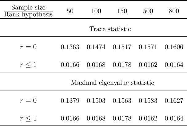
the trace and the maximal eigenvalue statistics, for different sample sizes.
Table 1. Rejection frequencies using the trace and
the maximal eigenvalue statistics (DGP1).
Sample size
Rank hypothesis 50 100 150 500 800
Trace statistic
r= 0 0.1363 0.1474 0.1517 0.1571 0.1606
r≤1 0.0166 0.0168 0.0178 0.0162 0.0164
Maximal eigenvalue statistic
r= 0 0.1379 0.1503 0.1563 0.1583 0.1627
r≤1 0.0166 0.0168 0.0178 0.0162 0.0164
Table 2. Rejection frequencies using the trace and
the maximal eigenvalue statistics (DGP2).
Sample size
Rank hypothesis 50 100 150 500 800
Trace statistic
r= 0 1 1 1 1 1
r≤1 0.0747 0.0686 0.0669 0.0722 0.0686
Maximal eigenvalue statistic
r= 0 1 1 1 1 1
[image:19.612.151.461.447.654.2]>From Table 1 we can see that the tests might not detect any cointegrating vectors
(low rejection frequencies of r = 0, especially for small sample sizes) which is what
we expected since (r−k) = 0 (see Section III). From Table 2 we conclude that with
DGP2 the LR tests are very likely to detect one cointegrating vector and this is in
accordance with the theoretical finding which suggests that if (r−k)> 0 the tests
detect at least(r−k) (2-1=1, in this case) cointegrating vectors.
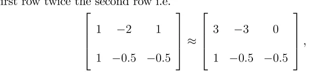
The following Monte Carlo experiments use a very large T value to evaluate the
probability limits of β˜ andα˜. We use a modified form of DGP2, in particular we use
a matrix whose rows are linear transformations of the rows of β0 found by adding to
thefirst row twice the second row i.e.
1 −2 1
1 −0.5 −0.5 ≈
3 −3 0
1 −0.5 −0.5 ,
where≈denotes a row equivalent matrix. Based on the asymptotic analysis of Section
IV, if we omit variableX3twe should expect one cointegrating vector whose estimator
converges to the space spanned byβ11 in the notation of Section IV, and in this case
β011 = ·
3 −3 ¸
. Table 3 shows the quantiles of the elements of the estimated
cointegrating vector, β˜11=
˜
β(1)11
˜
β(2)11
(associated with the largest eigenvalue) and the
elements of the eigenvector corresponding to the smallest eigenvalue. In fact we use
the normalised form of the estimated cointegrating vector,β˜11 given in (13), in order
[image:20.612.113.423.357.429.2]a linear combination of it. The estimation is carried out usingT = 5,000 and 10,000
[image:21.612.105.504.213.578.2]replications.
Table 3. Quantiles of the elements of
the estimated eigenvectors.
ˆ
v‡
Quantiles β˜ (1) 11 β˜
(2)
11 vˆ12 vˆ22
1% 2.9999 -3.0001 -0.0303 -0.0315
5% 3.0000 -3.0000 -0.0186 -0.0219
10% 3.0000 -3.0000 -0.0127 -0.0157
25% 3.0001 -2.9999 -0.0058 -0.0057
50% 3.0001 -2.9999 0.0001 -0.0000
75% 3.0003 -2.9997 0.0061 0.0053
90% 3.0005 -2.9995 0.0133 0.0151
95% 3.0007 -2.9993 0.0194 0.0209
99% 3.0011 -2.9989 0.0296 0.0321
‡Note. The first column of ˆv =
˜
β(1)11 vˆ12
˜
β(2)11 vˆ22
holds the eigenvector which corresponds
to the largest eigenvalue, i.e. the normalised estimated cointegrating vector, β˜11 whereas
In Table 3 we can see that the elements of the estimated cointegrating vector,
after normalisation converge to the appropriate elements of the submatrix of β in
the DGP namelyβ011=
·
3 −3 ¸
. The elements of the other estimated eigenvector,
which is associated with the smallest eigenvalue seem to be sufficiently small.
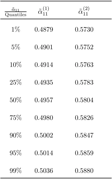
Next we use DGP2 and a SM with only X1t and X2t to compute the quantiles
of the elements of the estimated adjustment coefficient matrix. The estimator of α11
used in the simulations is given by α˜11 = ˆα11βˆ
0
11β¯11 (Section IV) which is a
trans-formation of αˆ11 such that α˜11β˜
0
11 = ˆα11βˆ
0
11. For T = 5,000 and 10,000 replications
the estimated adjustment coefficients seem to converge to the sum of the true
ad-justment coefficient matrix (i.e. the part ofα, α11 say, in the DGP that corresponds
to the single cointegrating vector that can be detected using the misspecified SM)
and the asymptotic bias. For this case we have α11 =
α(1)11
α(2)11
=
0.433
0.5 , and
˜
α11 =
˜
α(1)11
˜
α(2)11
Table 4. Quantiles of the estimated
adjustment coefficients.
˜ α11
Quantiles α˜ (1)
11 α˜
(2) 11
1% 0.4879 0.5730
5% 0.4901 0.5752
10% 0.4914 0.5763
25% 0.4935 0.5783
50% 0.4957 0.5804
75% 0.4980 0.5826
90% 0.5002 0.5847
95% 0.5014 0.5859
99% 0.5036 0.5880
Table 4 provides an illustration of Proposition 3 namely that the estimator of
the adjustment coefficients in an underspecified SM is inconsistent or asymptotically
biased. From Table 4 we can see that the normalised estimated adjustment coefficients
are biased upwards.
An empirical example
To illustrate the issue of omitted variables we use the four-equation system of
data6 are quarterly, seasonally adjusted, covering the period 1963Q1-1986Q2 on the
following variables: nominal M1 (M), real totalfinal expenditure at 1985 prices (I),
total final expenditure deflator (P) with 1985 as the base year, three-month local
authority interest rate (R1) and learning-adjusted interest rate on checking accounts
at commercial banks (R2). In the analysis the differenceR =R1−R2 is used instead
of theR1orR2 individually. The logarithms of the above variables are denoted by the
corresponding lower case letters. The interrelations among these variables have been
investigated extensively in the literature (see inter alia, Hendry and Mizon, 1993;
Hendry and Doornik, 1994; Ericsson et al., 1998; Doornik et al., 1998).
Following Doornik et al. (1998), there are two anticipated cointegrating relations
(m−p)t=c01+c11it+c21∆pt+c31Rt (15)
it=c02+c12t+c22∆pt+c32Rt (16)
thus equation (15) imposes long-run price homogeneity and equation (16) has a linear
trend (t) that captures exogenous technical progress. c11 is expected to be positive
and it can possibly be restricted to c11 = 1, making (15) a relation in the inverse
velocity of money. c21, c31 are expected to be negative. In (16) c22 and c32 are
expected to be positive and negative respectively.
6The data set is supplied with PcGive 10.0. The numerical results were obtained using PcGive
For the particular sample the variables (m−p)t, it, ∆pt andRt were found to be
I(1)(the results of unit root tests are omitted for the sake of brevity).
The first SM (SM1) is a VAR(3) in all four variables, (m − p)t, it, ∆pt and
Rt, which includes also an unrestricted constant, a restricted time trend and two
unrestricted dummy variables that account for shocks in output and prices. This
formulation was used by Doornik et al. (1998). The second SM (SM2) is the same
as the first (a VAR(3)) except that the potentially relevant variable Rt is omitted.
Rt enters both anticipated cointegrating relations and if both of them exist in the
DGP (and therefore can be detected by the tests with high probability) cointegration
tests should detect one cointegrating relation when Rt is omitted. This follows from
the asymptotic analysis and the evidence from the simulations. The third SM (SM3)
is the same as SM1 (again a VAR(3)) except that the variable (m−p)t is omitted.
The omitted variable in this case appears in only one of the anticipated cointegrating
relations therefore its omission should not affect the detection of the cointegrating
relation that does not involve (m−p)t, provided that both anticipated relations are
present in the DGP.
Tables 5, 6 and 7 show the statistics and p-values of the system diagnostic tests
Table 5. System diagnostic tests for SM1
Test Test Statistic p-value
Autocorrelation F(80, 254)=1.14 0.23
Normality χ2(8)=15.04 0.06
[image:26.612.187.426.278.392.2]Heteroscedasticity F(260, 503)=0.75 0.99
Table 6. System diagnostic tests for SM2
Test Test Statistic p-value
Autocorrelation F(45, 217)=1.22 0.18
Normality χ2(6)=7.60 0.27
Heteroscedasticity F(120, 377)=0.78 0.94
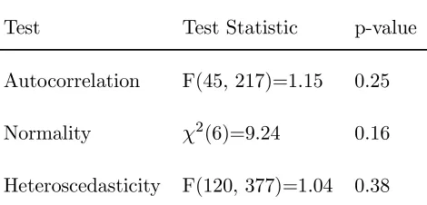
Table 7. System diagnostic tests for SM3
Test Test Statistic p-value
Autocorrelation F(45, 217)=1.15 0.25
Normality χ2(6)=9.24 0.16
Heteroscedasticity F(120, 377)=1.04 0.38
Thefirst diagnostic test is a Lagrange Multiplier test for 5-th order residual vector
autocorrelation, the second is a vector normality test and the third test is a vector
[image:26.612.190.425.438.551.2]tests do not indicate any source of misspecification. The omission of a potentially
relevant variable does not seem to affect the statistical adequacy of SM2 and SM3.
Tables 8, 9 and 10 report the results of cointegration tests for SM1, SM2 and SM3
respectively. Rejection of the null hypothesis at 1% level of significance is indicated
[image:27.612.151.463.272.409.2]by **.
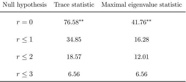
Table 8. Cointegration tests for SM1
Null hypothesis Trace statistic Maximal eigenvalue statistic
r= 0 76.58∗∗ 41.76∗∗
r≤1 34.85 16.28
r≤2 18.57 12.01
[image:27.612.149.464.470.567.2]r≤3 6.56 6.56
Table 9. Cointegration tests for SM2
Null hypothesis Trace statistic Maximal eigenvalue statistic
r= 0 38.37 18.18
r≤1 20.19 12.11
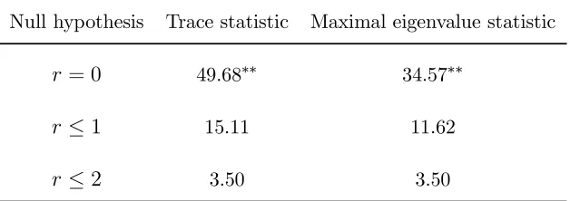
Table 10. Cointegration tests for SM3
Null hypothesis Trace statistic Maximal eigenvalue statistic
r= 0 49.68∗∗ 34.57∗∗
r≤1 15.11 11.62
r≤2 3.50 3.50
For SM1 the hypothesis that r= 0is rejected by both the trace and the maximal
eigenvalue tests. Therefore only one of the two anticipated cointegrating relations can
be detected by the tests. Since the cointegrating vectors are not identified it cannot
be determined at this stage which of the equations (15) or (16) the cointegrating
vector corresponds to. When the relevant variable Rt is omitted and SM2 is used
for cointegration testing neither the trace nor the maximal eigenvalue test rejects the
hypothesis thatr= 0. Hence, in the three-variable system no cointegrating relations
can be detected. Thisfinding was somehow expected given the result of cointegration
tests for SM1 and given the fact that both (15) and (16) include the omitted variable
Rt. However, the omission of(m−p)tdoes lead to rejection of the hypothesisr= 0in
the three-variable system. In this case the tests seem to detect the second anticipated
cointegrating relation.
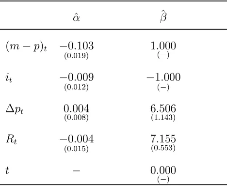
Carrying out restricted estimation of the cointegrating vectors, it is found that the
single cointegrating vector in SM1 is identified as the first anticipated cointegrating
the second anticipated relation given by (16). In SM1 the coefficient of the linear
trend is restricted to 0 and the coefficient of it is restricted to -1. The test statistic
for these restrictions is χ2(2) = 0.617 with p-value equal to 0.734. The results of
the restricted estimation appear in Table 11. In SM3 the coefficient of the trend is
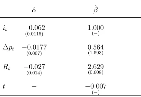
restricted to -0.007 which is the negative of the mean of∆it and the test statistic is
χ2(1) = 1.112 with p-value equal to 0.291. The results of the restricted estimation
appear in Table 12. Thus, in SM3 cointegration tests detect the second anticipated
cointegrating relation given by (16) which the former possibly lack power to detect
in SM1. Even though the results of the diagnostic tests of Table 7 do not indicate
[image:29.612.189.423.435.627.2]any misspecification in SM3, the sign and the significance of ∆pt do give a hint.
Table 11. Estimates of restricted cointegrating
vector and adjustment coefficients for SM1.
ˆ
α βˆ
(m−p)t −0.103
(0.019)
1.000
(−)
it −0.009
(0.012) −1(−.000)
∆pt 0.004
(0.008) 6(1..506143)
Rt −0.004
(0.015)
7.155
(0.553)
t − 0.000
Table 12. Estimates of restricted cointegrating
vector and adjustment coefficients for SM3.
ˆ
α βˆ
it −0.062
(0.0116) 1.(000−)
∆pt −0.0177
(0.007)
0.564
(1.593)
Rt −0.027
(0.014) 2(0..629608)
t − −0.007
(−)
The empirical example shows that the diagnostic tests are not always of help in
pointing out misspecification due to omitted variables. This is because in an error
correction model the omitted variables bias depends on submatrices of α, α12 (see
(14) and proof of Proposition 3). Thus, if α12 = 0 i.e. the variables in the DGP do
not adjust to cointegrating relations that involve omitted variables, the bias is zero
and therefore omission of relevant variables from the system may not be reflected in,
for example autocorrelation in the residuals of the model.
VI. Concluding remarks
This paper has considered the effects of underspecifying (omission of relevant
vari-ables) the SM on the LR tests for cointegration proposed by Johansen (1988, 1996).
We showed that omitting relevant variables from the SM will lead to either no
or equal to the number of omitted variables (r ≤ k) or the detection of q < r
coin-tegrating relationships, if the true coincoin-tegrating rank is greater than the number of
omitted variables (r > k). In addition, the use of an underspecified SM does not
affect the consistency of the estimated cointegrating vectors since they still converge
to a subspace of sp(β) but it does affect the consistency of the estimators of the
adjustment coefficient matrix and variance of the errors.
The model used to investigate the effects of omitted variables is quite simple,
be-ing a VAR(1) without deterministic terms, in order to minimise the complexity of the
algebra involved. Since the effect of short-run dynamics is asymptotically negligible,
their inclusion in the model would not alter the asymptotic findings. Inclusion of
deterministic terms would require different scaling matrices that would take into
ac-count the deterministic direction in thep-dimensional space, however the asymptotic
results would remain unchanged.
Although the analytical results are asymptotic, small sample simulations show
that the theoretical findings also arise in sample sizes used in empirical work. The
empirical example also illustrates this point.
The omitted variables can also beI(0). Since the inclusion of a stationary variable
increases the dimensions of the cointegrating space by one, omission of only I(0)
variables will lead to the underestimation of the cointegrating rank by the number of
Overall we conclude that the omission of relevant variables from the SM leads to
misleading inference, especially when followed by tests for linear restrictions onαand
β conditional on the wrong cointegrating rank.
Appendix
Proof of Proposition 1.
Let the non-stationary direction for the process Xt∗ be B∗ which isp∗×pfor case
(i) and p∗ ×(p−q) for case (ii) (for the detailed form ofB∗ see under the relevant
cases in Section III). By application of the Functional Central Limit Theorem on (8)
and the Continuous Mapping Theorem (see (B.12) and Theorem B.5 in Johansen,
1996) we have
T−1/2B∗0X[∗T u]=T−1/2B∗
0
(C∗
[T u]
X
i=1
ε[T u]+C1∗(L)ε[T u])
d
→B∗0C∗W(u)
B∗0X¯∗ →d B∗0C∗
Z 1
0
W(u)du
and
T−1B∗0S11∗ B∗ = T−2B∗0
T X
t=1
(Xt∗−1−X¯∗)(Xt∗−1−X¯∗)0B∗ (17)
d
→B∗0C∗
Z 1
0
˜
WW˜0C∗0B∗du.
Case (i)
Since β(1)0X∗
t is not I(0), because of the omission of relevant variables, (6) is not
matrix ΥT =
T−1/2Ir 0
0 Ip−r
we obtain,
|Υ0TBT0 S∗(ζ)BTΥT|= ¯ ¯ ¯ ¯ ¯ ¯ ¯ ¯
T−1ζβ(1)0
S∗
11β
(1)+op(1) T−1ζβ(1)0
S∗
11β¯ (1)
⊥ +op(1)
T−1ζβ¯(1)0
⊥ S11∗ β
(1)+op(1) T−1ζβ¯(1)0
⊥ S11∗ β¯ (1)
⊥ +op(1) −
op(1) op(1)
op(1) op(1) ¯ ¯ ¯ ¯ ¯ ¯ ¯ ¯ (18)
=¯¯¯T−1ζB∗0S11∗ B∗+op(1)¯¯¯
where B∗ = ·
β(1) β¯(1)⊥
¸
, p∗ ×p. The second matrix in (18) is o
p(1) because its
blocks are products of averages of products of either two I(0) processes (S00∗ ) or an
I(0) and an I(1) process (B∗0
S∗
10), which are Op(1) (see (B.12) in Johansen, 1996),
thus after scaling byΥT they all become op(1).
Then we have
|Υ0TBT0 S∗(ζ)BTΥT|= ¯ ¯
¯T−1B∗0S11∗ B∗+op(1) ¯ ¯ ¯ d → ¯ ¯ ¯
¯ζB∗0C∗ Z 1
0
˜
WW˜0C∗0B∗du
¯ ¯ ¯
¯= 0 (19)
by (17).
Case (ii)
In what follows we will use the row equivalent form of β that appears in (3).
the upper right block of β0 is zero. Thus, β = β11
p∗×q
β12
p∗×(r−q)
β21
k×q
β22
k×(r−q)
=
β11 β12
0 β22
.
We then have the following partitions: β(1) = ·
β11 β12
¸
defined above and β(2) = "
β21
k×q
β22
k×(r−q)
# =
·
0 β22
¸
. Note that β11 must satisfy the condition β
0
11C∗ = 0
so thatβ011X∗ t =β
0
11C1∗(L)εt∼I(0), by (8).
Then (6) becomes
|BT0 S∗(ζ)BT|= ¯ ¯ ¯ ¯ ¯ ¯ ¯ ¯ ¯ ¯ ¯ ¯
ζβ011S∗
11β11 ζβ
0
11S11∗ β12 T−1/2ζβ
0
11S11∗ β¯ (1)
⊥
ζβ012S11∗ β11 ζ(β
0
12S11∗ β12+β
0
22β22) T−1/2ζ(β
0
12S11∗ β¯ (1)
⊥ +β
0
22β¯ (2)
⊥ )
T−1/2ζβ¯(1)0
⊥ S∗11β11 T−1/2ζ(¯β (1)0
⊥ S11∗ β12+ ¯β (2)0
⊥ β22) T−1ζ(¯β (1)0
⊥ S11∗ β¯ (1)
⊥ + ¯β
(2)0
⊥ β¯
(2) ⊥ ) −
β011S10∗ S∗− 1
00 S01∗ β11 β
0
11S10∗ S∗− 1
00 S01∗ β12 β
0
11S10∗ S∗− 1 00 S01∗ β¯
(1)
⊥
β012S∗
10S∗− 1
00 S01∗ β11 β
0
12S10∗ S∗− 1
00 S01∗ β12 β
0
12S10∗ S∗− 1 00 S01∗ β¯
(1)
⊥
¯
β(1)⊥ 0S∗
10S∗− 1
00 S01∗ β11 β¯ (1)0
⊥ S10∗ S∗− 1
00 S01∗ β12 β¯ (1)0
⊥ S10∗ S∗− 1 00 S01∗ β¯
(1) ⊥ ¯ ¯ ¯ ¯ ¯ ¯ ¯ ¯ ¯ ¯ ¯ ¯ . (20)
Since β012X∗
t is assumed to be I(1) the first term of (20) needs to be rescaled. Let
now ΥT =
Iq 0 0
0 T−1/2I
r−q 0
0 0 Ip−r then
¯ ¯ ¯ ¯ ¯ ¯ ¯ ¯ ¯ ¯ ¯ ¯
ζβ011S11∗ β11 op(1) op(1)
op(1) ζT−1β
0
12S11∗ β12+op(1) ζT−1β
0
12S11∗ β¯ (1)
⊥ +op(1)
op(1) ζT−1β¯
(1)0
⊥ S11∗ β12+op(1) ζT−1β¯ (1)0
⊥ S11∗ β¯ (1)
⊥ +op(1) −
β011S10∗ S∗− 1
00 S01∗ β11 op(1) op(1)
op(1) op(1) op(1)
op(1) op(1) op(1) ¯ ¯ ¯ ¯ ¯ ¯ ¯ ¯ ¯ ¯ ¯ ¯ = ¯ ¯ ¯ ¯ ¯ ¯ ¯ ¯
ζβ011S11∗ β11−β
0
11S10∗ S∗− 1
00 S01∗ β11 op(1)
op(1) ζT−1B∗0
S∗
11B∗ +op(1)
¯ ¯ ¯ ¯ ¯ ¯ ¯ ¯ (21)
where nowB∗ = ·
β12 ¯β(1)⊥
¸
, p∗×(p−q).
The op(1) blocks are blocks that were Op(1) before scaling by ΥT because they
were products of averages of products of either twoI(0)processes (β011S∗
10,S00∗ ) or an
I(0)and an I(1)process (B∗0
S∗
10, B∗
0
S∗
11β11).
Next we define
V ar
∆Xt
β0Xt =
Σ00 Σ0β
Σβ0 Σββ
.
In order tofind the limit of (21) we need the following:
S00∗ →p Σ∗00=H0Σ00H (22)
β011S10∗ →p Σ∗β
110 =H
0
Σβ0H (23)
β011S11∗ β11→p Σ∗β
11β11 =H
0
andS00
p
→Σ00,β
0
S10
p
→Σβ0 andβ
0
S11β
p
→Σββ by the Weak Law of Large Numbers
(see also Johansen, 1996, Lemma 10.3)). Thus,
|Υ0TB
0
TS∗(ζ)BTΥT|= ¯ ¯ ¯ ¯ ¯ ¯ ¯ ¯
ζβ011S∗
11β11−β
0
11S10∗ S∗− 1
00 S01∗ β11 op(1)
op(1) ζT−1B∗0
S∗
11B∗+op(1)
¯ ¯ ¯ ¯ ¯ ¯ ¯ ¯ d → = ¯ ¯ ¯ ¯ ¯ ¯ ¯ ¯
ζΣ∗
β11β11 −Σ
∗
β110Σ
∗−1
00 Σ∗0β11 0
0 ζB∗0
C∗R1
0 W˜W˜
0
duC∗0
B∗ ¯ ¯ ¯ ¯ ¯ ¯ ¯ ¯
=|ζΣ∗β11β11 −Σ∗β110Σ∗−001Σ∗0β11||ζB∗
0
C∗
Z 1
0
˜
WW˜0duC∗0B∗|= 0 (25)
by (22)-(24) for the first factor and by (17) for the second. ¥
Proof of Proposition 2.
The equations (5) and (6) have the same eigenvalues but (6) has eigenvectors
BT−1Vˆ where Vˆ = "
ˆ
βq p×q
ˆ
V2
p×(p−q)
#
is the matrix whose columns are the eigenvectors
of (5) andβˆq =Hβˆ11=
ˆ β11 0
. The eigenvalues of (6) converge to the eigenvalues
of (25). Thus, the space spanned by theq first eigenvectors of (6), which correspond
to the q largest eigenvalues, converges to the space spanned by vectors with zeros
sp(BT−1βˆq) =sp(BT−1β˜q) where β˜q =Hβ˜11 and
BT−1β˜q = ¯ β0
T1/2β0⊥
β˜q.
First we analyse block (1,1). Using the formula for the partitioned inverse we have,
(β0β)−1 =
(β011β11)−1[Iq+β
0
11β12Fβ
0
12β11(β
0
11β11)−1] −(β
0
11β11)−1β
0
11β12F
−Fβ012β11(β011β11)−1 F
where
F = [β022β22+β012β¯11⊥β011⊥β12]−1.
Thus,
(β0β)−1β0β˜q = A1 A2
where A1 =Iq−β¯
0
11β12Fβ
0
12β¯11⊥b1 andA2 =Fβ
0
12β¯11⊥b1.
Then we analyse β0⊥β˜q which appears in block (2,1). Partitioningβ0⊥ as in β⊥ = "
β(1)⊥ 0
(p−r)×p∗
β(2)⊥ 0
(p−r)×k #
we obtain
β0⊥β˜q = ·
β(1)⊥ 0 β(2)⊥ 0
¸ ˜ β11 0
=β(1)
0
⊥ β˜11=β (1)0
⊥ β¯11⊥b1
by the assumptionβ0β⊥ = 0(orβ0⊥β = 0) which gives
β0⊥β = ·
β(1)⊥ 0 β(2)⊥ 0
¸
β11 β12
0 β22
=
·
β(1)⊥ 0β11 β (2)0
⊥ β12+β (2)0
⊥ β22
and therefore β(1)⊥ 0β11= 0.
Thus,
BT−1β˜q =
Iq−β¯
0
11β12Fβ
0
12β¯11⊥b1
q×q
Fβ012β¯11⊥b1 (r−q)×q
T1/2β(1)0
⊥ β¯11⊥b1 (p−r)×q
. (26)
By the form of (25) the last two blocks of (26) should converge to zero (in other
words sp(BT−1β˜q) should converge to the space spanned by vectors with zeros in
the last (p−q) coordinates. A necessary condition for this is T1/2b 1
p
→ 0. Then
sp(BT−1β˜q) p
→sp(
Iq
0 ).
>From (13) we obtainT1/2(˜β
11−β11) = ¯β11⊥(T1/2b1)
p
→0and that(˜β11−β11) =
op(T−1/2). ¥
Proof of Proposition 3.
Using the full sample, (14) can be written as
∆X∗ =α11β
0
11X−∗1+α12Z−1+ε∗ (27)
where ∆X∗, X−∗1, ε∗ are p∗ ×T, Z−1 is (r−q)×T and they are the full sample
counterparts of ∆Xt∗,Xt∗−1,ε∗t and Zt−1 respectively.
Using the partitioned form of Xt andβ,
Σββ = V ar(β
0
Xt−1) =E(β
0
Xt−1X
0
=
E(β011Xt∗−1X∗
0
t−1β11) E(β
0
11Xt∗−1Z
0
t−1)
E(Zt−1X∗
0
t−1β11) E(Zt−1Z
0
t−1)
≡
Σ∗
β11β11 Σ
∗
β11Z
Σ∗
Zβ11 Σ∗ZZ
and the second equality follows from the fact that there are no deterministic terms
in the DGP.
Since β11 can be estimated consistently (see Proposition 2)
plimα˜11=plimS01∗ β11(β
0
11S11∗ β11)−
1 =plim[T−1∆X∗X∗0
−1β11(T− 1β0
11X−∗1X∗
0
−1β11)− 1]
where the second equality is due to the absence of deterministic terms in the SM.
Substituting for∆X∗ as it is given in (27) and using Slutsky’s Theorem,
plim α˜11 (29)
= α11+α12plim[(T−1Z−1X∗
0
−1β11)][plim(T−1β
0
11X−∗1X∗
0
−1β11)]−1
= α11+α12Σ∗Zβ11Σ∗−β111β11
and the probability limits equal the corresponding population moments since the
process β0Xt−1 (and therefore β11Xt∗−1 and Zt−1) is stationary and ergodic. (29)
shows thatα˜11 is ‘inconsistent’ (or asymptotically biased) unless α12= 0 or
plim(T−1Z
−1X∗
0
−1β11) = 0. A stronger condition to achieve consistency isZ−1X∗
0
−1β11=
0 i.e. Z−1 is orthogonal to X∗
0
For the estimator of the variance-covariance matrix of the errors (again using the
consistency ofβ˜11) we have
plimΛˆ∗ = plim[S00∗ −S01∗ β11(β011S11∗ β11)−1β011S10∗ ]
= plim(T−1∆X∗∆X∗0)
−plim[T−1∆X∗X−∗01β11(T−1β
0
11X−∗1X∗
0
−1β11)−1T−1β
0
11X−∗1∆X∗
0
]
= plimT−1∆X∗M∗∆X∗0
whereM∗ =I T−X∗
0
−1β11(β
0
11X−∗1X∗
0
−1β11)−1β
0
11X−∗1. Substituting for∆X∗using (27),
plimΛˆ∗ =plimT−1[α12Z−1M∗Z
0
−1α
0
12+α12Z−1M∗ε∗
0
+ε∗M∗Z−0 1α012+ε∗M∗ε∗0]
andM∗Z−01 can be viewed as the residuals from the regression ofZ
0
−1 onβ
0
11X−∗1. By
the Weak Law of Large Numbers we have
plim T−1Z−1M∗ε∗
0
=E(Z−1M∗ε∗
0
) = 0
sinceE(Z−1M∗ε∗
0
) =E[E(Z−1M∗ε∗
0
|Xt−1)] =E[Z−1M∗E(ε∗
0
|Xt−1)] = 0, whereXt−1
is the minimal σ-field generated by the random vector Xt−1. Furthermore,
plimT−1β011X−∗1ε∗
0
=E(β011X−∗1ε∗
0
) = 0
since E(β011X∗ −1ε∗
0
) = E[E(β011X∗ −1ε∗
0
|Xt−1)] = E[β
0
11X−∗1E(ε∗
0
|Xt−1)] = 0 (see also
footnote 3). Hence,
plimΛˆ∗ = plim(T−1ε∗ε∗0) +plim(T−1α12Z−1M∗Z
0
−1α
0
12) (30)
= Ω∗+α12(Σ∗ZZ −Σ∗Zβ11Σ
∗−1
β11β11Σ∗β11Z)α
0
since ε∗ and Z
−1 are stationary random variables and by the Weak Law of Large
Numbers the probability limits in (30) equal their corresponding population moments.
Therefore,Λˆ∗ is ‘inconsistent’ unlessα12 = 0. ¥
References
Andrade, I. C., O’Brien, R. J. and Podivinsky, J. M. (1994). ‘Cointegration tests
and mean shifts’, University of Southampton Department of Economics Discussion
Paper, USDP 9405.
Boswijk, P. and Franses, P. H. (1992). ‘Dynamic specification and cointegration’,
Oxford Bulletin of Economics and Statistics, Vol. 53, pp. 369-382.
Cheung, Y. W. and Lai, K. S. (1993). ‘Finite-sample sizes of Johansen’s likelihood
ratio tests for cointegration’, Oxford Bulletin of Economics and Statistics, Vol. 55,
pp. 313-328.
DeLoach, S. B. (2001). ‘More evidence in favor of the Balassa-Samuelson hypothesis’,
Review of International Economics, Vol. 9, pp. 336-342.
Doornik, J. A. (1999). Object-Oriented Matrix Programming using Ox version 2.1,
Timberlake Consultants Ltd, London and www.nuff.ox.ac.uk/Users/Doornik.
Doornik, J. A. and Hendry, D. F. (2001). Modelling Dynamic Systems Using PcGive,
Volume II (3rd edition), Timberlake Consultants Press, London.
Doornik, J.A., Nielsen, B. and Hendry, D.F. (1998). ‘Inference in cointegrating
Ericsson, N. R., Hendry, D. F. and Mizon, G. E. (1998). ‘Exogeneity, cointegration
and economic policy analysis’,Journal of Business and Economic Statistics, Vol. 16,
pp. 370-387.
Hendry, D. F. and Doornik, J. A. (1994). ‘Modelling linear dynamic econometric
systems’. Scottish Journal of Political Economy, Vol. 41, pp. 1-33.
Hendry, D. F. and Mizon, G. E. (1992). ‘Evaluating dynamic econometric models
by encompassing the VAR’. In Models, Methods and Applications of Econometrics:
Essays in Honor of A. R. Bergstrom, pp. 272-300, ed. P. C. B. Phillips. Blackwell,
Cambridge MA.
Johansen, S. (1988). ‘Statistical analysis of cointegration vectors’, Journal of
Eco-nomic Dynamics and Control, Vol. 12, pp. 231-254.
Johansen, S. (1991). ‘Estimation and hypothesis testing of cointegration vectors in
gaussian vector autoregressive models’, Econometrica, Vol. 59, pp. 1551-1580.
Johansen, S. (1996). Likelihood-based Inference in Cointegrated Vector Autoregressive
Models, 2nd printing, Oxford University Press, Oxford.
Osterwald-Lenum, M. (1992). ‘A note with quantiles of the asymptotic
distribu-tion of the maximum likelihood cointegradistribu-tion rank test statistics’, Oxford Bulletin of
Economics and Statistics, Vol. 54, pp. 461-471.
Podivinsky, J. M. (1998). ‘Testing misspecified cointegrating relationships’.