An Interactive Fuzzy Satisficing Method for Multiobjective Operation Planning of District Heating and Cooling Plants Considering Contract Violation Penalties

An Interactive Fuzzy Satisficing Method for

Multiobjective Operation Planning of District

Heating and Cooling Plants Considering

Contract Violation Penalties

Masatoshi Sakawa

, Takeshi Matsui

, Keiichi Ishimaru

and Satoshi Ushiro

Abstract— District heating and cooling (DHC) sys-tems have been actively introduced as energy supply systems in urban areas. Since there exist a number of large-size freezers, heat exchangers and boilers in a DHC plant to generate and supply cold water, hot water and steam to a DHC system, the control un-der an operation plan for these instruments on the basis of the demand of cold water, hot water and steam, called heat load, is important for stable and economical management of DHC systems. In this paper, we formulate an operation planning problem of an actual DHC plant as a nonlinear integer pro-gramming problem in consideration of various penal-ties for violation of contracts. Furthermore, in order to reflect actual decision making situations for DHC plants more appropriately, we formulate a multiob-jective operation planning problem to minimize not only the running cost but the amount of primary ergy consumption from the viewpoint of saving en-ergy. Then, we propose an interactive fuzzy satis-ficing method through tabu search for multiobjective operation planning problems to derive a satisficing solution for the decision maker.

Keywords: interactive fuzzy satisficing method, district heating and cooling system, operation planning, con-tract violation penalty

1

Introduction

District heating and cooling (DHC) systems have been actively introduced as an energy supply system in urban areas for the purpose of saving energy, saving space,

in-∗_{Graduate School of Engineering, Hiroshima University,}

1-4-1, Kagamiyama, Higashi-Hiroshima, Hiroshima, 739-8527, JAPAN Email: [email protected]

†_{Graduate School of Engineering, Hiroshima University,}

1-4-1, Kagamiyama, Higashi-Hiroshima, Hiroshima, 739-8527, JAPAN Tel: +81-82-424-7695 Fax: +81-82-424-7195 Email: [email protected]

‡_{Urban Facilities Division, Shinryo Corporation, 3-7-1}

Nishish-injuku, Shinjuku-ku, Tokyo, 163-1021, JAPAN Email: [email protected]

§_{Urban Facilities Division, Shinryo Corporation, 3-7-1}

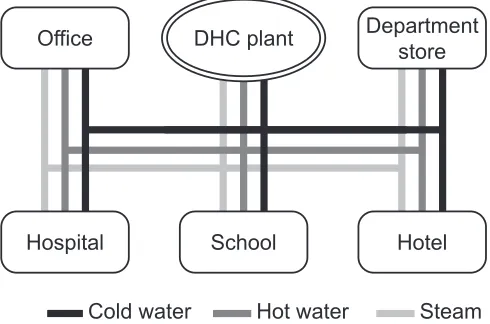
Nishishinjuku, Shinjuku-ku, Tokyo, 163-1021, JAPAN Email: [email protected]

Figure 1: An illustration of a district heating and cooling system.

hibiting air-pollution or preventing city disaster. In a typ-ical DHC system, cold water, hot water and steam used for air-conditioning at all facilities in a certain district are made and supplied by a DHC plant, as illustrated in Figure 1.

Since there exist a number of large-size freezers, heat ex-changers and boilers in a DHC plant, the control under an operation plan for these instruments on the basis of the amount of cold water, hot water and steam, called heat load, is important for stable and economical management of a DHC system.

In recent years, with the improvement of heat load pre-diction methods for DHC systems [3, 6], the needs of the formulation of operation planning problems of DHC plants as a mathematical programming one and the devel-opment of solution methods to the formulated problems has been increasing [2, 5, 7, 8, 10]. In previous researches [5, 7], the running cost involving the electric power rate and the gas rate based on the meter rate contract and the arrangement cost of instruments was considered as an objective function to be minimized in operation planning problems in DHC plants. However, actual DHC plant

op-IAENG International Journal of Applied Mathematics, 40:3, IJAM_40_3_11

eration companies have other contracts except the meter rate contract with the electric power company and the gas company. Therefore, we should incorporate penal-ties for violation of contracts into the running cost to estimate the running cost more accurately. In addition, these companies need to minimize not only the running cost but the energy consumption itself from the viewpoint of the energy saving.

Under these circumstances, in this paper, after formulat-ing an operation plannformulat-ing problem of a DHC plant in con-sideration of contract violation penalties, we formulate a multiobjective operation planning problem to simultane-oously minimize the running cost and the amount of pri-mary energy consumption from the viewpoint of saving energy. Then, we propose an interactive fuzzy satisfic-ing method through tabu search to derive a satisficsatisfic-ing solution for the decision maker and show its efficiency through numerical experiments using actual data.

2

Operation Planning of DHC Plants

2.1

Structure of a DHC Plant

A DHC plant usually generates cold water, hot water and steam by running many instruments using gas and electricity.

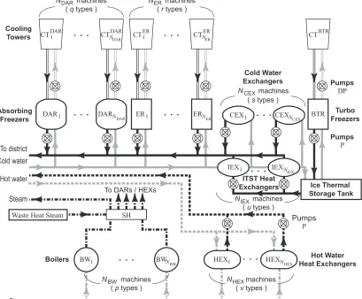
Relations among instruments in a DHC plant are de-picted in Figure 2. From Figure 2, it can be seen that hot water, steam required for heating and cold water required for cooling are generated by running NBW boilers of p

types, NDAR absorbing freezers of q types, NER turbo

freezers ofr types,NCEX cold water heat exchangers of s types,NIEX ice thermal storage heat exchangers ofu

types, NHEX hot water heat exchangers of s types and

a thermal storage tank using gas and electricity in this DHC plant, where pumps and cooling towers are con-nected with the corresponding freezers.

For the DHC plant, we need to find an optimal operation plan to minimize the cost of gas and electricity under the condition that the demand for cold water, hot water and steam must be satisfied by running instruments.

2.2

Problem Formulation

Given the (predicted) amount of the demand for cold water Cload(t), that for hot water Wload(t) and that for

steam Sload(t) at timet, the operation planning problem

of the DHC plant can be summarized as follows.

(I) The problem involves p + q + r + s +

u + v + 1 integer decision variables. Deci-sion variables (xt

1, . . . , xtq), (xtq+1, . . . , xtq+r),

(xt

q+r+1, . . . , xtq+r+s), (xtq+r+s+1, . . . , xtq+r+s+u) and

(xt_q+r+s+u+1, . . . , xt_q+r+s+u+v) are corresponding to the number of running instruments of absorbing freezers, that of turbo freezers, that of cold water heat exchangers,

that of ice thermal storage tank heat exchangers and that of hot water heat exchangers, while y1t, . . . , ytp are

that of boilers. In addition, there exists a decision variablezt_{which indicates whether some condition holds}

or not.

(II) The freezer output load rateP = (Ct_load−Ct T S)/Ct,

which means the ratio of the difference between the (pre-dicted) amount of the demand for cold water Cload(t)

and the output of the thermal storage tank which is au-tomatically running,Ct

T S, to the total output of running

freezersCt=∑_iq₌₁+r+s+uaixti, must be less than or equal

to 1.0, i.e.,

Ct≥Ct_load−C_{T S}t (1) where we denote the rating output of theith freezer byai.

This constraint means that the total output of running freezers and heat exchangers must exceed the necessary amount of cold water generated in the plant, Ct_load−C_{T S}t .

(III) The freezer output load rateP = (Ctload−CT St )/C t

must be greater than or equal to 0.2, i.e.,

0.2·Ct≤Ct_load−C_{T S}t . (2)

This constraint means that the total output of running freezers must not exceed five times the difference between the (predicted) amount of the demand for cold water and the output of the thermal storage tank.

(IV) The hot water heat exchanger output load rate

R = Wt_load/Wt_{, which means the ratio of the}

(pre-dicted) amount of the demand for hot water Wload(t)

to the total output of running heat exchangers Wt =

∑q+r+s+u+v

i=q+r+s+u+1bixti, must be less than or equal to 1.0,

i.e.,

Wt≥Wtload (3)

where we denote the rating output of the ith heat ex-changer bywi. This constraint means that the total

out-put of running hot water heat exchangers must exceed the (predicted) amount of the demand for hot water.

(V) The boiler output load rateQ= (St_DAR+St_HEX+ St_load−St_WHS)/St, which means the ratio of the necessary amount of steam generated in the plant to the total out-put of running boilersSt=∑p_j=1fjytj must be less than

or equal to 1.0, i.e.,

−S_DARt −S_HEXt +St≥St_load−St_WHS (4)

where we denote the rating output of the jth boiler by

fj. Furthermore,SDARt andSHEXt mean the total amount

of steam used by absorbing freezers at time t, defined as

S_DARt =

q

∑

i=1

Θ(P)·S_imax·xi (5)

and the total amount of steam used by heat exchangers at timet, defined as

SHEXt =Wt/0.95 (6)

IAENG International Journal of Applied Mathematics, 40:3, IJAM_40_3_11

Figure 2: Structure of a district heating and cooling plant.

IAENG International Journal of Applied Mathematics, 40:3, IJAM_40_3_11

whereS_imaxis the maximal steam amount used by theith absorbing freezers. In addition, StWHSmeans the amount

of waste heat steam supplied from the outside of this DHC system. Θ(P) is the rate of use of steam in an absorbing freezer, which is a nonlinear function of the freezer output load rate P in general. For the sake of simplicity, in this paper, we use the following piecewise linear approximation.

Θ(P) =

{

0.8775·P+ 0.0285 , P ≤0.6

1.1125·P−0.1125 , P >0.6 (7)

(VI) The boiler output load rateQ= (St

DAR+SHEXt +

St_load−St_WHS)/St must be greater than or equal to 0.2, i.e.,

−SDARt −SHEXt + 0.2·St≤S t load−S

t

WHS. (8)

This constraint means that the total output of running boilers must not exceed five times the necessary amount of steam.

(VII) The minimizing objective functionJ(t) is the

en-ergy cost which is the sum of the gas bill and the elec-tricity bill.

J(t) = Gcost·AtG+ Ecost·AtE (9)

where Gcost and Ecost are the unit cost of gas and that

of electricity, respectively.

The gas consumption At_G is defined as the gas amount consumed in the rating running of a boiler gj, j =

1,2, . . . , pand the boiler output load rateQ.

At_G =

 

p

∑

j=1 gjyj



_·Q (10)

On the other hand, the electricity consumption At E is

defined as the sum of electricity amount consumed by turbo freezers, accompanying cooling towers and pumps.

AEt = EERt +ECTt +EDPt +EPt

=

q+r

∑

i=1

Ξ(P)·Eimax·xti+ q+r

∑

i=1 cCTi xti

+

q+r

∑

i=1

cDP_i xt_i+

q+r+_∑s+u+v

i=1

cP_i xt_i (11)

whereEmax

i denotes the maximal electricity amount used

by the ith turbo freezer, cCT

i , cDPi and cPi are the

elec-tricity amount of cooling tower and those of two kinds of pumps.

In the above equation, Ξ(P) denotes the rate of use of electricity in a turbo freezer, which is a nonlinear func-tion of the freezer output load rate P. For the sake of

simplicity, in this paper, we use the following piecewise linear approximation.

Ξ(P) =

{

0.6·P+ 0.2 , P ≤0.6

1.1·P−0.1 , P >0.6 (12)

Accordingly, the operation planning problem is formu-lated as the following nonlinear integer programming problem.

ProblemP(t)

minimize

J(xt,yt, zt) = Gcost·AtG+ E t cost·A

t

E (13)

subject to

−(1−zt)·(Ct−(Ctload−CT St ))≤0 (14) zt·(0.2·Ct)+ (1−zt)·(0.6·Ct)

≤Ct_load−C_{T S}t (15)

−zt·(0.6·Ct−(Ctload−CT St )

)

≤0 (16)

−Wt≤ −Wt_load (17)

zt·Θ1(P) + (1−zt)·Θ2(P) +SHEXt −S t

≤ −Stload+ S t

W HS (18)

−zt·Θ1(P)−(1−zt)·Θ2(P)−SHEXt + 0.2·S t

≤St_load−St_{W HS} (19)

xt_i∈ {0,1, . . . , NDARi}, i= 1, . . . , q (20)

xt_i∈ {0,1, . . . , NERi}, i=q+ 1, . . . , q+r (21)

xt_i∈ {0,1, . . . , NCEXi},

i=q+r+ 1, . . . , q+r+s (22)

xt_i∈ {0,1, . . . , NIEXi},

i=q+r+s+ 1, . . . , q+r+s+u(23)

xt_i∈ {0,1, . . . , NHEXi},

i=q+r+s+u+ 1, . . . , q+r+s+u+v(24)

yt_j∈ {0,1, . . . , NBWj}, j = 1, . . . , p (25)

zt∈ {0,1} (26)

where

Ct=

q+r

∑

i=1

aixti, W t₌

q+r+_∑s+u+v

i=q+r++s+u+1 bixti,

St=

p

∑

j=1

fjyjt, P = (C t load−C

t T S)/C

t_,

Θ1(P) = q

∑

i=1

(0.8775·P+ 0.0285)·S_imax·xt_i,

Θ2(P) = q

∑

i=1

(1.1125·P−0.1125)·S_imax·xt_i,

Ξ1(P) = q+r

∑

i=q+1

(0.6·P+ 0.2)·E_imax·xt_i,

IAENG International Journal of Applied Mathematics, 40:3, IJAM_40_3_11

Ξ2(P) = q+r

∑

i=q+1

(1.1·P−0.1)·E_imax·xt_i,

At_G=

 

p

∑

j=1 gjyjt

 _·Q,

Q= (1/St){zt·Θ1(P) + (1−zt)·Θ2(P)

+S_HEXt + St_load−St_WHS},

AtE= {

zt·Ξ1(P) + (1−zt)·Ξ2(P)

+

q+r

∑

i=1

cCT_i xt_i+

q+r

∑

i=1

cCP_i xt_i+

q+r+_∑s+u+v

i=1

cCDP_i xt_i }

.

In the problem,zt_{= 1,z}t_{= 0 meanP ≤0.6,P >0.6,}

re-spectively. In the following, letλt=

(

(xt₎T_,(yt₎T_{, z}t)T

and let Λt_{be the feasible region ofP(t).}

Since an operation plan for one day is usually made in the DHC plant operation company every day, we should consider 24-hour operation plans λ(0,24) = ((λ0)T_,(λ1

)T_{, . . . ,(λ}23

)T_{)∈Λ(0,24) = Λ}0_×Λ1_{× · · · ×}

Λ23_{. Thus, Sakawa et al. [5, 7] studied multi-period}

op-eration planning problems to reflect the practical situa-tion for DHC plants. In multi-period operasitua-tion plans, we must consider the switching of instruments since instru-ments running in the previous period may be stopping in the next period, and vice versa. Since the starting and stopping of instruments need more electricity and man-power than the continuous running does, the arrangement cost of instruments should be took into account in multi-period operation planning.

Thus, they formulated an extended operation planning problem in consideration of the arrangement cost of in-struments [5, 7]. To be more specific, we deal with the following problem P(0,24) for 24-hour operation plan-ning.

Extended problemP(0,24)

minimize

J0,24(λ(0,24)) =J(λ0) + 23 ∑

τ=1 [

J(λτ)

+

p+q+r_∑+s+u+v

j=1

ϕjλτj −λ (τ−1) j

]

(27)

subject to

λ(0,24)∈Λ(0,24) (28)

where ϕj is the cost of switching of thejth instrument.

In should be noted thatP(0,24) is a large-scale nonlinear integer programming problem which involves 24 times as many variables asP(t) does.

3

Contract Violation Penalties and

Mul-tiobjective Problem

The DHC plant operation company considered in this paper has the following contracts except the meter rate contract with the electric power company and the gas company.

• Least gas consumption contract: The DHC

plant operation company has a least gas consump-tion contract with the gas company, where the amount of gas consumption of a year must be greater than or equal to a fixed value B1. If the amount of

gas consumption of a year is less than B1, the DHC

plant operation company must pay the penalty M1

to the gas company.

• Greatest electric power contract: The DHC

plant operation company has a greatest electric power contract with the electric power company, where the electric power at any time must be less than or equal to a fixed value B2. If the electric

power exceeds B2 at some time, the DHC plant

op-eration company must pay the penalty M2 to the

electric power company.

• Peak cut contract: The DHC plant operation

company has a peak cut contract with the electric power company, where the electric power in the peak period from 13:00 to 16:00 must be less than or equal to a fixed value Bt₃. If the electric power exceeds Bt₃ in the peak period, the DHC plant operation com-pany must pay the penalty M3 to the electric power

company.

If any contract is violated, the DHC company has to pay the penalty.

Now, we give mathematical expressions of penalties men-tioned above. First, we consider the penalty of the great-est electric power contract, PE2(·), and that of the peak

cut contract, PE3(·). Either the greatest electric power

contract or that of the peak cut contract is violated when the electric power exceeds B2or B3. Then, the DHC

com-pany has to pay M2or M3. Thus, we define them as:

PE2(λt) = {

M2 , ifAtE>B2,

0 , otherwise

PE3(λt) = {

M3 , ifAtE>B t

3, tin the peak period,

0 , otherwise

Next, we consider the penalty of the least gas consump-tion contract. Let αm, m = 1,2, . . . ,12 be the ratio

of monthly gas consumption to yearly gas consumption for each month.For a monthly operation plan from the first day (day 1) to the last day (day dm) of month

IAENG International Journal of Applied Mathematics, 40:3, IJAM_40_3_11

m, we define monthly thresholds B1,m, m= 1,2, . . . ,12

as B1,m = B1 · αm. In addition, we define monthly

penalties of the least gas consumption contract, PE1,m, m= 1,2, . . . ,12 as M1,m= M1·αm.Then, based on the

gas consumption from day 1 to day d of month m and the number of remaining days of monthm,dm−(d−1),

we define the daily threshold of daydas:

B1,m(d) =

B1,m−AG(d−1) dm−(d−1)

where

AG(d) = d·24 ∑

τ=1  ∑p

j=1 gjyjτ

 _·Q.

Since the daily threshold B1,m(d) increases as the total

gas consumption from day 1 to day d of month m de-creases, it can reflect the situation of gas consumption on dayd.

We also define the daily penalty of day das:

M1,m(d) =

M1,m dm−(d−1)

.

Then, we can define the penalty of the least gas con-sumption contract for a 24-hour operation plan λ(0,24) as:

PE1(λ(0,24)) =     

M1,m(d) , if 23 ∑

τ=0

Aτ_G<B1,m(d)

0 , otherwise

Introducing these penalties into the objective function of

P(0,24), we extend P(0,24) into the following problem with penalties.

Extended problem with penaltiesP′(0,24)

minimize

J₀′_,24(λ(0,24)) =J0,24(λ(0,24)) + PE1(λ(0,24))

+

23 ∑

τ=0

[PE2(λτ) + PE3(λτ)] (29)

subject to λ(0,24)∈Λ(0,24) (30)

Furthermore, in order to reflect actual decision making situations for DHC plants more appropriately, we formu-late a multiobjective extended problem to minimize not only the running cost but the amount of primary energy consumption from the viewpoint of saving energy during

D days.

Multiobjective extended problemM OP′(0,24, D)

minimize

J1′(λ(0,24), . . . ,λ(24(D−1),24))

=

D_∑−1

d=0 {

J24d,24(λ(24d,24)) + PE1(λ(24d,24))

+

23 ∑

τ=0 [

PE2(λ24d+τ) + PE3(λ24d+τ) ]}

(31)

minimize

J₂′(λ(0,24), . . . ,λ(24(D−1),24))

=

D∑−1

d=0 { ₂₃

∑

τ=0

αG·A24Gd+τ+αEA24Ed+τ }

(32)

subject to

λ(24d,24)∈Λ(24d,24), d= 0,1, . . . , D−1 (33)

whereαGandαEare the coefficient of conversion to

pri-mary energy for gas and that for electricity, respectively.

4

An

Interactive

Fuzzy

Satisficing

Method

In order to consider the imprecise nature of the deci-sion maker’s judgments for each objective functionJ_l′(·),

l = 1,2, if we introduce the fuzzy goals such as “J_l′(·) should be substantially less than or equal topl”, the

mul-tiobjective extended problem can be transformed as:

maximize µ1(J1′(λ(0,24), . . . ,λ(24(D−1),24)))

maximize µ2(J₂′(λ(0,24), . . . ,λ(24(D−1),24))) subject to

λ(24d,24)∈Λ(24d,24), d= 0,1, . . . , D−1

       (34) whereµl(Jl′(·)) are membership functions to quantify the

fuzzy goals.

As a reasonable solution concept for the fuzzy multiobjec-tive decision making problem, Sakawa et al. [4, 9] defined M-Pareto optimality on the basis of membership func-tion values and developed an interactive fuzzy satisfic-ing method to derive a satisficsatisfic-ing solution guaranteed to be M-Pareto optimal by eliciting the local preference in-formation from the decision maker through interactions. In their method [4, 9], the decision maker interactively updates aspiration levels of achievement for membership values of all fuzzy goals, called reference membership lev-els, until he is satisfied. To be more specific, for the deci-sion maker’s reference membership levels ¯µlthe following

augmented minimax problem is repeatedly solved:

minimize

max

l=1,2 {(

¯

µl−µl(Jl′(λ(0,24), . . . ,λ(24(D−1),24)))

) +ρ 2 ∑ i=1 ( ¯

µi−µi(Ji′(λ(0,24), . . . ,λ(24(D−1),24)))

)}

subject to

λ(24d,24)∈Λ(24d,24), d= 0,1, . . . , D−1

                     (35)

IAENG International Journal of Applied Mathematics, 40:3, IJAM_40_3_11

whereρis a sufficiently small positive number. If the ref-erence membership levels are not attainable, the optimal solution to (35) is the nearest feasible solution to them in the augmented minimax sense. Otherwise, the optimal solution to (35) could be better than them.

In this paper, we apply and adjust the interactive fuzzy satisficing method to the above multiobjective extended problem (34).

Interactive fuzzy satisficing method forM OP′(0,24, D)

Step 1 In order to obtain the minimum J′_l and

(ap-proximate) maximum J′_l of J_l′(·), l = 1,2 in

M OP′(0,24, D), solve (36) and (37).

minimize J_l′(λ(0,24), . . . ,λ(24(D−1),24)) subject to

λ(24d,24)∈Λ(24d,24), d= 0,1, . . . , D−1

  

(36) maximize J_l′(λ(0,24), . . . ,λ(24(D−1),24)) subject to

λ(24d,24)∈Λ(24d,24), d= 0,1, . . . , D−1

  

(37)

Step 2 Ask the decision maker to specify membership

functions µl(Jl′(·)), l = 1,2 based on minima and

maxima obtained in step 1, and set the initial refer-ence membership levels ¯µl,l= 1,2.

Step 3 For the current reference membership levels

(¯µ1,µ2¯ ), solve the corresponding augmented mini-max problem (35). It should be noted that the opti-mal solution to (35) is M-Pareto optiopti-mal.

Step 4 If the decision maker is satisfied with the current

solution obatined in step 3, the interaction process is terminated. Otherwise, ask the decision maker to update ¯µl, l = 1,2 in consideration of the current

membership function values and objective function values, and go to step 3.

Since problems (36), (37) and (35) are large-scale nonlin-ear integer programming problems, it is difficult to find an exact optimal solution to it. Thus, we use an approx-imate solution method using tabu search. To be more specific, we extend the tabu search based on strategic os-cillation for multidimensional integer knapsack problems [1] to nonlinear integer programming problems and apply it to solve (36), (37) and (35).

5

Tabu Search Based on Strategic

Oscil-lation

In this paper, we extend tabu search based on strategic oscillation for multidimensional 0-1 knapsack problems [1] to nonlinear integer programming problems. The tabu

search proposed in [1] made use of the property of mul-tidimensional 0-1 knapsack problems that the improve-ment or disimproveimprove-ment of the objective function value corresponds with the decrease or increase of the degree of feasibility. From the property, it is clear that the optimal solution to multidimensional 0-1 knapsack problems ex-ists in the area near the boundary of the feasible region which is called the promising zone. Thus, the search di-rection in multidimensional 0-1 knapsack problems can be controlled by checking the change of the objective func-tion value. In the case of nonlinear integer programming problems, the promising zone does not always exist near the boundary of the feasible region since the monotone relation between the objective function value and the de-gree of feasibility no longer holds. Since the promising zone originally means the area which is considered to in-clude an optimal solution, we define the promising zone for nonlinear integer programming problems as neighbor-hoods of local optimal solutions. Thus, in order to use not only the change of the objective function value but the degree of feasibility, we introduce the index of sur-plus of constraints δ(λ(t,24)) and that of slackness of constraintsϵ(λ(t,24)).

                  

δ(λ(t,24))=△

t_∑+23

τ=t

∑

i∈I+

gτ_i(λτ),

I+_{={i |g}τ i(λ

τ_{)>0, i∈ {1, . . . ,8}}}

ϵ(λ(t,24))=△

t_∑+23

τ=t

∑

i_∈I−

−giτ(λ τ

),

I−={ i|gτ i(λ

τ

)≤0, i∈ {1, . . . ,8}}

where gt

i(·) ≤ 0, i ∈ {1,2, . . . ,8} correspond with

con-straints inP(t).

Step 0: INITIALIZATION

Generate an initial solutionλ(t,24) at random, and ini-tialize the tabu list TL, parameters CN, DN and AN. Ifλ(t,24) is feasible, go to step 4. Otherwise, go to step 1.

Step 1: TS PROJECT

The aim of this step is to move the current solution in the infeasible region to the promising zone in the gentlest ascent (disimproving) direction about the objective func-tion with decreasing the surplus of constraintsδ(λ(t,24))

While δ(λ(t,24)) is positive, i.e., the current solution is infeasible, repeat finding a non-tabu decision variable which decreasesδ(λ(t,24)) and gives the lest disimprove-ment of the objective function value when its value would be changed, changing the value of the decision variable actually and adding the decision variable to TL. If there does not exist any non-tabu decision variable that de-creases δ(λ(t,24)), select a decision variable randomly, change its value even ifδ(λ(t,24)) increases and add the decision variable to TL. Ifδ(λ(t,24)) = 0 and there does not exist any decision variable which improves the objec-tive function value by changing its value, go to step 2.

IAENG International Journal of Applied Mathematics, 40:3, IJAM_40_3_11

Step 2: TS COMPLEMENT

The aim of this step is to search the promising zone in-tensively.

Letλ′(t,24) :=λ(t,24) andλ′′(t,24) :=λ′(t,24). Then, select several tabu decision variables of λ′′(t,24) and change their values. If δ(λ′′(t,24)) = 0, then carry out step 4. Otherwise, carry out step 1. IfJ_t,′₂₄(λ′′(t,24))< J_t,′₂₄(λ(t,24)) for the solution δ(λ′′(t,24)) obtained by step 4 or step 1, letλ(t,24) :=λ′′(t,24). This procedure is repeatedCN times. If the previous step of this step is step 1, then go to step 3. If the previous step of this step is step 4, then go to step 5.

Step 3: TS DROP

The aim of this step is to move the current solution in the promising zone to the inside of the feasible region in the gentlest ascent direction of the objective function with increasing the slackness of constraintsϵ(λ(t,24))

Repeat finding a non-tabu decision variable which in-creases ϵ(λ(t,24)) and gives the lest disimprovement of the objective function when its value would be changed, changing the value of the decision variable actually and adding the decision variable to TL. If there does not exist any non-tabu decision variable that increases ϵ(λ(t,24)) or the number of repetitions of the above procedure ex-ceedsDN, go to step 4.

Step 4: TS ADD

The aim of this step is to move the current solution in the feasible region to the promising zone in the steepest de-scent (improving) direction about the objective function with keepingδ(λ(t,24)) = 0.

Whileδ(λ(t,24)) = 0, i.e., the current solution is feasible, repeat finding a non-tabu decision variable which keeps

δ(λ(t,24)) = 0 and gives the greatest improvement of the objective function value when its value would be changed, changing the value of the decision variable actually and adding the decision variable to TL. If there does not exist such a decision variable, go to step 2.

Step 5: TS INFEASIBLE ADD

The aim of this step is to move the current solution in the promising zone to the infeasible region in the steepest de-scent (if exist) or the gentlest ade-scent direction about the objective function with decreasing the slackness of con-straintsϵ(λ(t,24)) or increasing the surplus of constraints

δ(λ(t,24)).

Repeat finding a non-tabu decision variable which de-creasing the slackness of constraintsϵ(λ(t,24)) or increas-ing the surplus of constraints δ(λ(t,24)) and gives the greatest improvement (if exist) or the lest disimprove-ment of the objective function value when its value would be changed, changing the value of the decision variable actually and adding the decision variable to TL. If there does not exist such a decision variable or the number of repetitions of the above procedure exceedsAN, go to step 1.

Table 1: Individual minima J_l,′_min and maxima J_l,′_max,

l= 1,2

Objective function J_l,′_min J_l,′_max J₁′ 465294344.9 150878375.0

J₂′ 329818346.2 120242558.1

6

Numerical Experiments

In this section, we deal with an actual DHC plant with boilers of 3 types, absorbing freezers of 4 types, turbo freezers of 4 types, cold water heat exchangers of 2 types, ice thermal storage tank heat exchangers of 2 types and heat exchangers of 3 types. Thus, a daily (24-hour) op-eration planning problem for a certain day for this plant involves 456 integer decision variables.

Here, we consider monthly operation planning with two objective functions of this DHC plant. After formulating it as a multiobjective extended problemM OP′(0,24, D) which includes 456×31 integer decision variables, we apply the proposed interactive fuzzy satisficing method through the tabu search. The problem involves two ob-jective functions: the running costJ₁′(·) and the amount of primary energy consumptionJ₂′(·).

Numerical experiments are carried out on a personal com-puter (CPU:Intel PentiumIV Processor 2.40GHz, Mem-ory: 512MB, C Compiler: Microsoft Visual C++ 6.0) and the number of trials of tabu search is 10.

First, according to step 1 in the interactive fuzzy satisfic-ing method, we calculate the (approximate) minimum of

J_l,′_min and the (approximate) maximum J_l,′_max, l = 1,2. Table 1 shows these values.

Second, according to step 2, the hypothetical decision maker specifies membership functionsµl(·),l= 1,2 based

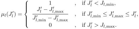
on the individual minima and maxima of objective func-tionsJ_l′(·). In this experiment, we use linear membership functions defined as:

µl(Jl′) =

      

1 , ifJ_l′< Jl,min, J_l′−J_l,′_max

J_l,′_min−J_l,′_max , ifJ

′

l,min≤Jl,′max≤Jl′,

0 , ifJ_l′> Jl,max.

Then, the decision maker sets the initial reference mem-bership levels (¯µ1,µ¯2) = (1.00,1.00).

Next, according to step 3, the augmented minimax prob-lem (35) for the current reference membership levels is solved by the tabu search. The results are shown in the second column of Table 2.

In step 4, since the decision maker cannot be satisfied with this result and he/she feels that J₁′ should be im-proved even ifJ₂′ becomes worse, the reference member-ship levels are updated from (1.00,1.00) to (1.00,0.95),

IAENG International Journal of Applied Mathematics, 40:3, IJAM_40_3_11

Table 2: Interaction process

Interaction 1st 2nd 3rd

¯

µ1 1.00 1.00 1.0 ¯

µ2 1.00 0.95 0.9

µ1 0.63 0.66 0.71

µ2 0.65 0.64 0.61

J₁′ 263358375.0 248088543.1 219563349.5

J₂′ 185391644.7 195669214.1 213127596.4

and return to step 3.

Again, the minimax problem (35) is solved for the current reference membership levels, and the results are shown in the third column of Table 2.

Furthermore, the decision maker hopes thatJ1′ becomes

better at the additional expense ofJ₂′ and updates the ref-erence membership levels from (1.00,0.95) to (1.00,0.90). The results are shown in the fourth column of Table 2.

In this experiment, since the decision maker is satisfied with this result, this solution is the satisficing solution for the decision maker, and the interaction process stops.

7

Conclusion

In this paper, we focused on operation planning of dis-trict heating and cooling (DHC) plants considering con-tracts with the electric power company and the gas com-pany except the meter rate contract. First, we formu-lated a single period operation planning problem P(t) and a multi-period operation planning problem P(0,24) as a nonlinear integer programming problem. Second, in consideration of penalties for violation of contracts, we formulated an extended multi-period operation planning problem with the penalties P′(0,24). Next, in order to reflect actual decision making situations for DHC plants more appropriately, we formulate a multiobjective oper-ation planning problemM OP′(0,24, D) to minimize not only the running cost but the amount of primary energy consumption from the viewpoint of saving energy dur-ing D days. Then, we dicussed the application of an interactive fuzzy satificing method through tabu search into multiobjective operation planning problems to de-rive a satisficing solution for the decision maker. Finally, we show the feasibility and usefulness of the interactive method for multiobjective operation planning problems through a numerical experiment using actual data.

References

[1] S. Hanafi and A. Freville, “An efficient tabu search approach for the 0-1 multidimensional knapsack problem,” European Journal of Operational Re-search, V106, N2–3, pp. 659–675, 4/98.

[2] D. Henning, S. Amiri, and K. Holmgren, “Modelling and optimisation of electricity, steam and district heating production for a local Swedish utility,” Eu-ropean Journal of Operational Research, V175, N2, pp. 1224–1247, 9/06.

[3] K. Kato, M. Sakawa, K. Ishimaru, S. Ushiro, and T. Shibano, “Heat load prediction through recur-rent neural network in district heating and cooling systems,” 2008 IEEE International Conference on Systems, Man and Cybernetics (SMC 2008), Suntec, Singapore, pp. 1401–1406, 10/08.

[4] M. Sakawa,Fuzzy Sets and Interactive Multiobjective Optimization, Plenum Press, 1993.

[5] M. Sakawa, K. Kato, S. Ushiro, and M. Inaoka. “Operation planning of district heating and cool-ing plants uscool-ing genetic algorithms for mixed integer programming,”Applied Soft Computing, V1, N2, pp. 139–150, 8/01.

[6] M. Sakawa, K. Kato, and S. Ushiro, “Cooling load prediction in a district heating and cooling system through simplified robust filter and multi-layered neural network,”Applied Artificial Intelligence: In-ternational Journal, V15, N7, pp. 633–643, 8/01.

[7] M. Sakawa, K. Kato, and S. Ushiro, “Opera-tion planning of district heating and cooling plants through genetic algorithms for nonlinear 0-1 pro-gramming,” Computers & Mathematics with Appli-cations, V42, N10–11, pp. 1365–1378, 11-12/01.

[8] M. Sakawa, T. Matsui, K. Ishimaru and S. Ushiro, “An Interactive Fuzzy Satisficing Method for Mul-tiobjective Operation Planning of District Heat-ing and CoolHeat-ing Plants ConsiderHeat-ing Various Penal-ties for Violation of Contract,” Lecture Notes in Engineering and Computer Science: Proceedings of The International MultiConference of Engineers and Computer Scientists 2010, IMECS 2010, 17-19 March, 2010, Hong Kong, pp2127-2133.

[9] M. Sakawa, H. Yano and T. Yumine, “An inter-active fuzzy satisficing method for multiobjective linear-programming problems and its application,” IEEE Transactions on Systems, Man, and Cyber-netics, VSMC-17, N4, pp. 654–661, 4/87.

[10] R. Yokoyama and K. Ito, “A revised decomposition method for MILP problems and its application to operational planning of thermal storage systems,” Journal of Energy Resources Technology, V118, pp. 277–284, 12/96.

IAENG International Journal of Applied Mathematics, 40:3, IJAM_40_3_11