The Bloom Paradox:
When
not
to Use a Bloom Filter
Ori Rottenstreich and Isaac Keslassy
Abstract—In this paper, we uncover the Bloom paradox in Bloom filters: sometimes, the Bloom filter is harmful and should not be queried.
We first analyze conditions under which the Bloom paradox occurs in a Bloom filter, and demonstrate that it depends on the a priori probability that a given element belongs to the represented set. We show that the Bloom paradox also applies to Counting Bloom Filters (CBFs), and depends on the product of the hashed counters of each element. In addition, we further suggest improved architectures that deal with the Bloom paradox in Bloom filters, CBFs and their variants. We further present an application of the presented theory in cache sharing among Web proxies. Last, using simulations, we verify our theoretical results, and show that our improved schemes can lead to a large improvement in the performance of Bloom filters and CBFs.
Index Terms—The Bloom Filter Paradox, Bloom Filter, Count-ing Bloom Filter,A PrioriMembership Probability.
I. INTRODUCTION
A. The Bloom Paradox
Bloom filters are widely used in many networking device al-gorithms, in fields as diverse as accounting, monitoring, load-balancing, policy enforcement, routing, filtering, security, and differentiated services [1]–[6]. Bloom filters are probabilistic data structures that can answer set membership queries without false negatives (if they indicate that an element does not belong to the represented set, they are always correct), but also with low-probability false positives (they might sometimes indicate that an arbitrary element is a member of the represented set although it is not). In addition, Bloom filters have many variants. In particular, Counting Bloom Filters (CBFs) add counters to the Bloom filter structure, thus also allowing for deletions within counter limits.
Networking devices typically use Bloom filters ascache di-rectories. Bloom filters are particularly popular among design-ers because a Bloom filter-based cache directory has no false negatives, few false positives, and O(1)update complexity.
In this paper, we show that the traditional approach to this Bloom-based directory forgets to take into account the a priori set-membership probabilityof the elements, i.e. the set-membership probabilitywithout such a directory. Surprisingly, forgetting this a priori probability can actually make the directory more harmful than beneficial.
Figure 1(a) illustrates the intuition behind the importance of thea prioriset-membership probability. Consider a generic system composed of a user, a main memory containing all the
O. Rottenstreich and I. Keslassy are with the Department of Electrical Engineering, Technion, Haifa 32000, Israel (e-mails: [email protected], [email protected]).
(a) Illustration of the importance of thea prioriset-membership probability. When the user needs elementx(illustrated as an arrival of a query forx), there are two options. First, to access the main memory with a fixed cost of 10. Second, to look for it in the cache. With some probability, it is indeed there and the cost is only1. With the complementary probability, it is not there and the user has to also access the main memory with a total cost of 1 + 10 = 11.
(b) Illustration of the elements in the cache C, those with a positive membership indication in the Bloom Filter B, and those in the memory M. With a false positive probability of10−3, a positive indication of the Bloom
[image:1.612.317.561.173.265.2]filter isincorrectw.p. |B|B\C|| ≈10710−7104 = 1−10−3≈1. Fig. 1. Illustration of the Bloom paradox.
data, and a cache with a subset of the data. When the user needs to read a piece of data, it can simply access the main memory directly, with a cost of10. Alternatively, it can also access the cache first, with a cost of1. If the cache owns this piece of data, there is no additional cost. Else, it also needs to access the main memory with an additional cost of10. This is a generic problem, where the costs may correspond todollar amounts (e.g. for an ISP customer that either accesses a cached Youtube video at the ISP cache, or the more distant Youtube server), to power (e.g. in a two-level memory system or a two-level IP forwarding system within a networking device), or tobandwidth(e.g. in a data center, with a local cache in the same rack as a server versus a more distant main memory).
he pays just above 1 on average, since he will most often pay 1 (with probability 1−10−3), and rarely 1 + 10 = 11
(with probability 10−3). If instead he directly accesses the
main memory, he always pays 10.
However, this approach completely disregards the a pri-ori probability, and it is particularly wrong if the a priori probability is too small. For instance, assume that the main memory contains1010elements, while the cache only contains 104 elements. For simplicity, further assume that xis drawn
uniformly at random from the memory, i.e., the a priori probability that it belongs to the cache is 104/1010= 10−6.
This is the probabilitybeforewe query the Bloom filter. Then the probability that x is in the cache after the Bloom filter says it is in the cache is only about ≈ 10−6/10−3 = 10−3
(the exact computation is in the paper).
This is theBloom paradox: with high probability (1−10−3),
x is actually not in the cache, even though the Bloom filter indicates thatxisin the cache. More generally, if thea priori probability is low enough before accessing the Bloom filter, it is better to disregard the Bloom filter results and always go automatically to the main memory — in fact, in this case the Bloom filter is harmful and it is better to not even query the Bloom filter. Taken to the extreme, when the Bloom paradox applies to all elements, it means in fact that the entire cache is useless.
Figure 1(b) provides a more formal view to this Bloom paradox. Let B be the set of elements with a positive membership indication from the Bloom filter. Then, |B| = 104 + 10−3·(1010−104) ≈ 107. While the false positive
rate of the Bloom filter is ||MB\\CC||= 10−3, the probability that a positive indication is incorrect is significantly larger and equals |B|B\C|| ≈10710−7104 = 1−10−3.
Of course, in the general case, different assumptions may weaken or even cancel the Bloom paradox, especially when caches have significantly non-uniforma prioriprobabilities.
B. Contributions
The main contribution of this paper is pointing out the Bloom paradox, and providing a first analysis of its conse-quences on Bloom filters and Counting Bloom Filters (CBFs). First, in Section IV, we provide simple criteria for the existence of a Bloom paradox in Bloom filters. In particular, we develop an upper bound on the a priori probability under which the Bloom paradox appears and the Bloom filter answer is irrelevant. Based on this observation, we suggest improvements to the implementation of both the insertion and the query operations in a Bloom filter.
Then, in Section V, we focus on CBFs. We observe that we can calculate a more accurate membership probability based on the exact values of the counters provided in a query, and provide a closed-form solution for this probability. We further show how to use this probability to obtain a decision that optimizes the use of a CBF in a generic system. We also discuss the effect of the number of hash functions on the CBF performance.
Next, in Section VI, we generalize our analysis to other variants of the Bloom filter and in particular the Bh−CBF
scheme [5].
Later, in Section VII, we consider a distributed-cache ap-plication with several proxies that use CBFs to represent their cache contents. We suggest an optimal order of the queries that should be sent to the proxies in this network.
Last, in Section VIII, we evaluate our optimization schemes, and show how they can lead to a significant performance improvement. Our evaluations are based on synthetic data as well as on real-life traces.
II. RELATEDWORK
The Bloom filter data structure (and its variants) has a long list of applications in the networking area [7]. This includes, for instance, cache digests [2], packet classification [8], rout-ing [9], deep packet inspection [10], security [11] and state representation [12]. Bloom Filters and CBFs can be found in such well-known products as Facebook’s distributed storage system Cassandra [13], Google’s web browser Chrome [14] and the network storage system Venti [15].
Different design schemes have been suggested to improve the false positive rate of CBFs with a limited memory size. For instance, the MultiLayer Hashed CBF performs a hierarchical compression [16]. A related approach is presented in [17], [18]. Memory-efficient schemes based on fingerprints instead of on counters were suggested in [3], [12]. TheBh−CBF [5]
is a recent efficient CBF variant based on variable increments. In all these variants, false negatives are prohibited and only false positives are allowed.
In [19], Donnetet al.presented the Retouched Bloom Filter (RBF), a Bloom Filter extension that reduces its false positive rate at the expense of random false negatives by resetting selected bits. The authors also suggested several heuristics for selectively clearing several bits in order to improve this tradeoff. For instance, choosing the bits to reset such that the number of generated false negatives is minimized, or alternatively, the number of cleared false positives is maxi-mized. They also show that randomly resetting bits yields a lower bound on the performance of their suggested schemes. Unfortunately, calculating the optimal selection of bits can be prohibitive (for instance, it requires going over all the elements in the universe several times), and in practice only approximated schemes are used.
Laufer et al. presented in [20] a similar idea called the Generalized Bloom Filter (GBF) in which at each insertion, several bits are set and others are reset, according to two sets of hash functions. To examine the membership of an element, a match is required in all corresponding hash locations of both types. False negatives can occur in case of bit overwriting during the insertions of later elements. On the one hand, increasing the number of hash functions reduces the false positive rate, since more bits are compared. On the other, it increases the false negative rate due to a higher probability of bit overwriting. Data structures with false positives as well as false negatives have also been discussed in [21].
TABLE I
MEMBERSHIPQUERYDECISIONCOSTS FOR AN ELEMENTx∈U
Positive Membership Negative Membership
Decision Decision
x∈S WP= 0 WF N=α·WF P
x /∈S WF P WN= 0
not exist. Consider for instance, a variant of the Web proxy application from [2] in which Bloom filters are used to summarize the content of each cache. If a large memory with all elements does not exist and each data element can be found in at most one of the caches, false negatives can eliminate the possibility to find a queried element. Another application is in Bloom-filter-based forwarding [22], [23]. Bloom filters are used to encode a delivery tree as a set of forwarding-hop identifiers, e.g. links or pairs of adjacent links in the tree. While false positives can just cause a short increase in the delay, false negatives may prevent the packet from reaching its destination.
The issue of wrongly considering the a prioriprobabilities is a known problem in diverse fields. For instance, the Prose-cutor’s Fallacy[24] is a known mistake made in law when the prior odds of a defendant to be guilty before an evidence was found are neglected. The same problem is also known as the False Positive Paradox in other fields such as computational geology [25], and is also related to Probabilistic Primality Testing[26]. Our results might apply to such problems when the costs of false negatives and false positives are taken into account. We leave these to future work.
III. MODEL ANDNOTATIONS
We consider a Bloom filter (or alternatively a Counting Bloom Filter (CBF)) representing a setSofnelements taken from a universe U of N elements. The Bloom filter uses m bits, and relies on a set ofkhash functionsH ={h1, . . . , hk}.
For each elementx∈U, we denote byPr(x∈S)thea pri-oriprobability thatx∈S, i.e. the probability before we query the Bloom filter. We further denote byPr (x∈S|BF= 1)the probability that x ∈ S given that the Bloom filter indicates so, where BF is the indicator function of the answer of the Bloom filter to the query of whetherxis a member ofS.
We assume that the cost function of an answer to a member-ship query can have four possible values. They are summarized in Table I, which illustrates these costs for a query of an element x ∈ U. If x ∈ S, the cost of a positive (correct) decision is WP while the cost of negative (incorrect) decision
is WF N. Similarly, if x /∈ S, the costs are WF P and WN
for a positive and negative decision, respectively. In the most general case, the costs of the two correct decisions, WP and WN might be positive. However, we can simply reduce the
problem to the case where WP = WN = 0 by considering
only the marginal additional costs of a negative incorrect decision and a positive incorrect decision (WF N−WP)and
(WF P −WN). Finally, for WF P >0 let α denote the ratio WF N/WF P. The variableαrepresents how expensive a false
negative error is in comparison with a false positive error. In the suggested analysis, we assume for the sake of simplic-ity uniformly-distributed and independent hash functions. We
also assume that the number of hash functions in the Bloom filter and the Counting Bloom filter is the optimal number k ≈ ln(2)·(m/n). Accordingly, the probability of a bit to be set after the insertion of the n elements is 0.5. These assumptions often appear in the literature, e.g. in [3], [27], [28]. Of course, in practicek has to be integer and thus the probability of 0.5 is approximated. Likewise, the requirement for independency between the hash functions can be slightly relaxed while keeping the same asymptotic error [29]. We also assume that each hash function has a range ofm/kentries that are disjoint from the entries for the other hash functions. This common implementation is described in [7] and is shown to have the same asymptotic performance.
Our goal is to minimize the expected cost in each query decision, therefore we return a negative answer iff its expected cost is smaller than the cost of a positive answer.
IV. THEBLOOMPARADOX INBLOOMFILTERS
In this section we develop conditions for the existence of the Bloom paradox in Bloom filters. We also provide improvements to the implementation of both the insertion and the query operations in a Bloom filter.
A. Conditions for the Bloom Paradox
The next theorem expresses the maximal a priori set-membership probability of an element such that the Bloom filter is irrelevant in its queries. This bound depends on the error cost ratio α and on the bits-per-element ratio of the Bloom filter, which impacts its false positive rate.
Intuitively, in cases where the Bloom filter indicates that the element is in the cache, a smallerα=WF N/WF P means that
the cost of a false negative is relatively smaller, and therefore we would prefer a negative answer in more cases, i.e., even for elements with a higher a priori probability. Therefore, a smallerαallows for the Bloom paradox to occur more often, and in particular also given a higher a prioriprobability.
Theorem 1: The Bloom filter paradox occurs for an element xif and only if itsa priorimembership probability satisfies
Pr(x∈S)< 1
1 +α·2ln(2)·(m/n)
Proof:We compare the expected cost of positive and neg-ative answers in case the Bloom filter indicates a membership and show that for a lowa priorimembership probability, the cost of a positive answer can be larger. The Bloom paradox occurs when a negative answer should be returned even though the Bloom filter indicates a membership. In order to choose the right answer, we first calculate the conditioned membership probability whenBF= 1. First,
Pr(x∈S|BF= 1) = Pr(x∈S,BF= 1) Pr(BF= 1) =
Pr(x∈S) Pr(BF= 1),
because by definition a Bloom filter always returns 1 for an element in the set S, i.e.Pr(BF= 1|x∈S) = 1. Likewise,
Pr(x /∈S|BF= 1) = 1−Pr(x∈S|BF= 1)
ForBF= 1, letE1(x)denote the expected cost of a positive
decision for an element x, andE0(x)for a negative decision.
Then,
E1(x) = Pr (x /∈S|BF= 1)·WF P
= Pr(BF= 1)−Pr(x∈S) Pr(BF= 1) ·WF P,
and
E0(x) = Pr (x∈S|BF= 1)·WF N =
Pr(x∈S)
Pr(BF= 1)·WF N.
The Bloom paradox occurs when E1(x)> E0(x), i.e
Pr(BF= 1)−Pr(x∈S)
Pr(BF= 1) ·WF P >
Pr(x∈S)
Pr(BF= 1) ·WF N,
which can be rewritten as
Pr(BF= 1)>(α+ 1)·Pr(x∈S).
We use our model assumption that Pr(BF = 1) = (1/2)ln(2)·(m/n) if x /∈S. Also, Pr(BF = 1) = 1if x∈S.
Then, the left side of the last condition can be rewritten as (
(1/2)ln(2)·(m/n)·Pr(x /∈S) + 1·Pr(x∈S) )
, and we finally have
(1/2)ln(2)·(m/n)·(1−Pr(x∈S))> α·Pr(x∈S),
which provides the required result.
We refer to the inequality from Theorem 1 as the condition for the Bloom paradox.
B. Analysis of the Bloom Paradox
We now provide an illustration of the impact of various parameters on the Bloom paradox.
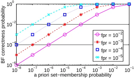
Figure 2(a) illustrates the probability that a Bloom filter is indeed correct when it indicates that an elementxis a member of the set. This probability,Pr (x∈S|BF= 1), depends on the a prioriset-membership probability of the elementPr(x∈S)
as well as on the false positive rate of the Bloom filter. For instance, if Pr(x∈S) = 10−6 and the false positive rate is 10−3, the Bloom filter is correct w.p. Pr (x∈S|BF= 1) =
Pr(x∈S) Pr(BF=1) =
10−6
10−3·(1−10−6)+1·10−6 ≈10−
6/10−3= 10−3.
Figure 2(b) plots the boundaries of the Bloom paradox. It presents the minimal bits-per-element ratio m/n needed to avoid the Bloom paradox, as a function of the a priori probability, given α= 0.1,1,10,100. For instance, ifα= 1, i.e. the costs of the two possible errors are equal, and the a priori probability isPr(x∈S) = 10−6, at leastm/n= 28.7
memory bits per element are required to consider the Bloom filter and avoid the Bloom paradox. If this ratio is smaller, the Bloom paradox occurs, so we should return a negative answer for all the queries of x, independently of the answer of the Bloom filter.
10−6 10−5 10−4 10−3 10−2 10−1 10−7
10−8 10−4 10−2 100
10−6
BF correctness probability
a priori set−membership probability fpr = 10−2 fpr = 10−3 fpr = 10−4 fpr = 10−5
(a) The Bloom filter correctness probability as a function of thea priori set-membership probability.
10−6 10−5 10−4 10−3 10−2 10−1 10−7
10−8 0 10 20 30 40 50
minimal m / n ratio
a priori set−membership probability
α = 0.1
α = 1
α = 10
α = 100
[image:4.612.324.545.56.184.2](b) Boundaries of the Bloom paradox: minimal number of bits-per-element for a Bloom filter to avoid the Bloom paradox, as a function of thea priori set-membership probability.
Fig. 2. Analysis of the Bloom paradox. (a) shows that a lowera priori probability makes the Bloom filter increasingly irrelevant, because the a posteriorimembership probability after the Bloom filter is positive is also lower. This favors the Bloom paradox. (b) provides the exact borders of the region in which the Bloom paradox occurs as a function of the a priori probability, the Bloom filter load, and the relative weights of false-positive and false-negative errors.
C. Bloom Filter Improvements Against the Bloom Paradox
Based on the observation in Theorem 1, we suggest the two following improvements to Bloom filters, as illustrated in Figure 3:
Selective Bloom Filter Insertion—If the a priori
proba-bility of an element x satisfies the condition for the Bloom paradox, we will not take the answer of the Bloom filter into account after the query. Therefore,it is better not to even insert it in the Bloom filter, so as to reduce the load of the Bloom filter. Therefore, the final numbern∗of inserted elements may satisfyn∗< n.
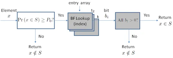
Selective Bloom Filter Query—If thea prioriprobability
of an elementxsatisfies the condition for the Bloom paradox, we do not want to take the answer of the Bloom filter into account, and therefore it is better to not even query it. Formally, ifPr(x∈S)< P0= (1+α·2ln(2)·(m/n
∗)
)−1, where
n∗ is the final number of inserted elements, then a negative answer should be returned for the queries of x, regardless of the Bloom filter.
(a) Selective Bloom Filter Insertion. Elements with lowa prioriset-membership probability are not in-serted into the Bloom filter.
[image:5.612.277.556.59.153.2](b) Selective Bloom Filter Query. Elements with lowa prioriset-membership probability are not even queried, as shown in the first rectangle, and a negative answer is always returned for them no matter what the Bloom filter would have actually stated.
Fig. 3. Logical view of the Selective Bloom Filter implementation. Components that also appear in a regular Bloom filter are presented in gray. (a) shows a first possible improvement during insertion, where elements that satisfy the condition for the Bloom paradox are not even inserted into the Bloom filter. (b) displays a second possible improvement during query, where elements that satisfy the condition for the Bloom paradox are not even queried.
filter load, leading to a lower false positive probability. In turn, implementing the Selective Bloom Filter Query alone makes a regular Bloom filter more efficient by discarding harmful query results for elements with low a priori probability. Finally, implementing both the Selective Bloom Filter Insertion and Query results in the strongest improvement that combines the benefits of both approaches. All these approaches are further compared using simulations in Section VIII.
Note that each of the two improvements requires knowing the a priori probabilities at different times (either during the insertion or during the query). Also, as expected, this approach may cause false negatives, since this may reduce the overall error cost.
D. Estimating the a PrioriProbability
Access patterns to caches tend to have the locality of reference property, i.e. it is more likely that recently-used data will be accessed again in the near future. Therefore, the a priori probability distribution might be significantly non-uniform over U.
In such cases, we suggest to estimate the a priori prob-ability by sampling arbitrary element queries and checking whether they belong to the cache. In practice, for 1% of element queries, we will check whether they belong to the cache, and use an exponentially-weighted moving average to approximate the a prioriprobability. Of course, the accuracy of the estimation depends on the sampling rate. The estimation accuracy as a function of the rate is discussed for instance in [30].
In addition, there might be several subsets of elements with clearly different a priori probabilities. For instance, packets originating from Class-A IP addresses might have distinct a priori probabilities from those with classes B and C. Then we will simply model thea prioriprobability as uniform over each class, and sample each class independently.
Besides sampling, analytical models have been proposed to predict the locality and the hit rate of a cache while considering its cache size and replacement policy [31]–[33]. For instance, [34] described a model based on the histogram of the time differences between two accesses to the same memory element.
V. THEBLOOMPARADOX IN THECOUNTINGBLOOM FILTER
A. The CBF-Based Membership Probability
In this section, we want to show the existence and the consequences of the Bloom paradox in Counting Bloom Filters (CBFs). To do so, we show how we can calculate the membership probability of an element in S based on the exact values of the counters of the CBF. We show again the existence of aBloom paradox: in some cases, a negative answer should be returned even though the CBF indicates that the element is inside that set. Finally, we prove a simple result that surprised us: to determine whether an element that hashes intok counters falls under the Bloom paradox, we only need to comparethe product of these counterswith a threshold, and do not have to analyze a full combinatorial set of possibilities.
For an elementx∈U, we denote byPr (x∈S|CBF)its membership probability inS, based on its CBF counter values. That is, on the values of the k counters with indices hj(x)
for j ∈ {1, . . . , k} pointed by the set of k hash functions {h1, . . . , hk}. Let C = (C1, . . . , Ck) denote the k counter
indices of x, i.e. Cj = hj(x) for j ∈ {1, . . . , k}, and let c= (c1, . . . , ck)denote the values of these counters.
Theorem 2: The CBF-based membership probability is
Pr (x∈S|CBF) =
mk·(∏kj=1cj)·Pr(x∈S)
mk·(∏k
j=1cj)·Pr(x∈S) + (n·k)k·(1−Pr(x∈S))
.
Proof: We again use Bayes’ theorem to calculate the conditioned membership probability while now considering the exact values of the k counters. Let X be an indicator variable for the event x ∈S such that X = 1 iff x∈ S. If cj = 0 for any j ∈ {1, . . . , k}, thenPr (x∈S|CBF) = 0.
have that
Pr (C=c|X = 1) =
k
∏
j=1
Pr (Cj =cj|X= 1)
=
k
∏
j=1 (
n−1
cj−1
)(k
m
)cj−1(
1− k
m
)n−cj
.
Likewise,
Pr (C=c|X = 0) =
k
∏
j=1
Pr (Cj =cj|X = 0)
=
k
∏
j=1 (
n cj
)(k
m
)cj(
1− k
m
)n−cj
and again Pr (X= 1) = Pr(x∈S)andPr (X= 0) = (1− Pr(x∈S)). Putting all together, we have
Pr (x∈S|CBF) = Pr (X = 1|C=c)
= Pr (C=c|X= 1) Pr (X= 1)
Pr (C=c|X= 1) Pr (X= 1) + Pr (C=c|X= 0) Pr (X= 0)
=
∏k
j=1
(n−1)!
(cj−1)!(n−cj)!Pr (X= 1)
∏k
j=1
(n−1)!
(cj−1)!(n−cj)!Pr (X= 1) +
∏k
j=1
( n!
cj!(n−cj)!·
k m )
Pr (X= 0)
= Pr (X = 1)
Pr (X = 1) +∏kj=1 (
n cj ·
k m
)
·Pr (X = 0)
= m
k·(∏k
j=1cj)·Pr(x∈S)
mk·(∏k
j=1cj)·Pr(x∈S) + (n·k)k·(1−Pr(x∈S)) .
Directly from the last theorem we can deduce the following corollary.
Corollary 3: For an elementx∈U, the CBF-based mem-bership probability Pr (x∈S|CBF) is an increasing func-tion of the product of the k counters pointed by hi(x) for i∈ {1, . . . , k}.
This result surprised us because of the simple dependency ofPr (x∈S|CBF)only in the product of thekcounters and not in a more complicated function of them.
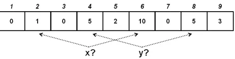
Example 1: Figure 4 illustrates queries of two elements x and y in a CBF with parameters of m, n and k. The values of the counters pointed by x are 1,10. Like-wise, they are 5,5 for y. Then, by Theorem 2 their CBF-based membership probabilities are Pr (x∈S|CBF) =
mk·(1·10)·Pr(x∈S)
mk·(1·10)·Pr(x∈S)+(n·k)k·(1−Pr(x∈S)) andPr (y∈S|CBF) =
mk·(5·5)·Pr(y∈S)
mk·(5·5)·Pr(y∈S)+(n·k)k·(1−Pr(y∈S)), respectively. In particular,
if they have the same a priori membership probabilities (i.e. Pr(x ∈ S) = Pr(y ∈ S)) then Pr (y∈S|CBF) >
Pr (x∈S|CBF)since5·5 = 25>10 = 1·10.
B. Optimal Decision Policy for a Minimal Cost
[image:6.612.319.550.53.111.2]We now suggest an optimal decision policy for the query of an element x ∈ U in a CBF. This policy relies on its
Fig. 4. Illustration of CBF queries of two elements x and y. Ifx and y have the same a priori membership probabilities then their CBF-based membership probabilities satisfies Pr (y∈S|CBF) > Pr (x∈S|CBF) since5·5 = 25>10 = 1·10.
Fig. 5. Logical view of the Selective Counting Bloom Filter implementation. Components that also appear in a regular CBF are presented in gray. Mem-bership probability is calculated based on the counters product. A negative answer is returned for elements with low calculated membership probability.
CBF-based membership probability, which was expressed in Theorem 2 as a function of the product of its counter values. Theorem 4: An optimal decision policy for the CBF is to be positive on the membership iff
Pr (x∈S|CBF)≥ 1
α+ 1.
Proof:We compare the expected cost of positive and neg-ative decisions given the conditioned CBF-based membership probability, and explain that a positive decision should be made only when the probability is beyond a given threshold. Let againE1(x)be the expected cost of a positive decision for an element x andE0(x) for a negative decision. For a positive decision, the cost isWP ifx∈S(w.p.Pr (x∈S|CBF)) and WF P ifx /∈S (w.p1−Pr (x∈S|CBF)). Thus, we have that
E1(x) = (1−Pr (x∈S|CBF))·WF P.
Likewise, we have an expected cost for a negative decision,
E0(x) = Pr (x∈S|CBF)·WF N.
To minimize the expected cost, the scheme decides on a positive answer ifE1(x)≤E0(x), i.e when
(1−Pr (x∈S|CBF))·WF P ≤Pr (x∈S|CBF)·WF N
With simple algebra, we can see that the last inequality holds if
Pr (x∈S|CBF)≥ 1
α+ 1.
[image:6.612.324.559.173.255.2]C. Optimal Number of Hash Functions
Given the parameters m, n of a Bloom filter (and a CBF as well), the number of hash functions k ≈ ln(2)·(m/n)
is typically chosen in order to minimize the false positive probability without false negatives. In the suggested schemes, the goal is different. Instead of minimizing the false positive probability, we try to minimize the expected cost of a query decision. Thus, the optimal number of hash functions is not necessarily k ≈ ln(2)·(m/n) anymore. According to the decision policy in the previous subsection, we present the expected cost as the function of the number of hash functions k, such that akthat minimizes this cost should be selected.
To do so, we define several new notations. We generalize the functionPr (x∈S|CBF)to be a function of the number of hash functions k and of the product π of these counters, while mandnare considered as constants, such that
P(x, k, π) = Pr
x∈S|k=k,
(∏k
j=1
cj
) =π
= m
k·π·Pr(x∈S)
mk·π·Pr(x∈S) + (n·k)k·(1−Pr(x∈S)).
Likewise, we generalize the function of the expected cost for both of the decisions. We define E0(x, k, π)and E1(x, k, π)
as the expected cost of negative and positive decisions for an element x when the number of hash functions is k and the product of the counters is π. Formally,
E0(x, k, π) =P(x, k, π)·WF N,
and
E1(x, k, π) = (1−P(x, k, π))·WF P.
We also define for x ∈ U and k hash functions, the value
Π(x, k) as the minimal value of π that yields a probability P(x, k, π)not smaller than the threshold1/(α+ 1), i.e.
Π(x, k) = min {
π∈N|P(x, k, π)≥ 1
α+ 1 }
.
Last, we define P(k, π) as the probability that the product of k counters, in a CBF is exactly π, where each counter is randomly picked in each sub-array of the CBF. It can be calculated as the sum of the probabilities for the vectors of counters with this property.
Then, we have that the expected cost function for a query of an element x∈U is:
E(x, k) =
Π(x,k∑)−1
π=0
P(k, π)·E0(x, k, π)
+
∞
∑
π=Π(x,k)
P(k, π)·E1(x, k, π).
Given the probability that a query is of a specific element x ∈ U denoted by PQ(x), the expected cost when k hash
functions are used is
E(k) =∑
x∈U
PQ(x)·E(x, k)
=∑
x∈U PQ(x)·
(Π(x,k)−1
∑
π=0
P(k, π)·E0(x, k, π)
+
∞
∑
π=Π(x,k)
P(k, π)·E1(x, k, π) )
.
Thus, the optimal number of hash functions is the value ofk that minimizes the last expression. In simulations, we discuss this further.
VI. THEBLOOMPARADOX INADDITIONALVARIANTS OF THEBLOOMFILTER
In this section, we examine the existence and the conse-quences of the Bloom paradox in an additional variant of the Bloom Filter and the Counting Bloom Filter. We consider the Bh−CBF scheme [5], a recently suggested improved
Count-ing Bloom Filter technique based on variable increments. The scheme makes use ofBhsequences. Intuitively, aBhsequence
is a set of integers with the property that for anyh′ ≤h, all the sums ofh′ elements from the set are distinct. Therefore, given a sum of up tohelements, we can calculate, for each element of theBh sequence, its multiplicity in the unique multiset of
addends from which the sum is comprised.
The Bh−CBF scheme includes a pair of counters in
each hash entry: one with fixed increments, and another one with variable increments that are selected from the Bh
sequence. For j ∈ [1, k], let cj and aj be the values of the
fixed-increment and variable-increment counters in the entry hj(x), respectively. Further, we denote the Bh sequence by D={v1, v2, ..., vℓ} such that|D|=ℓ. The Bh−CBF uses
two sets ofk hash functions. The first setH ={h1, . . . , hk}
useskhash functions with range{1, . . . , m}and points to the set of entries, as in the CBF. The second setG={g1, . . . , gk}
useskfunctions with range{1, . . . , ℓ}, i.e. it points to the set Dand determines the variable increment of an element in each of itskupdated counters.
For an element x ∈ U, we would like to calculate
Pr (x∈S|Bh−CBF), the membership probability of x
based on thekcorresponding hash entries of theBh−CBF. Theorem 5: Forj∈ {1, . . . , k}, letyjdenote the
multiplic-ity of vgj(x) in the addends of the sum aj. Further, let I(j)
be an indicator function representing whether cj ≤h. Then,
Pr (x∈S|Bh−CBF) =
mk·δ·Pr(x∈S)
mk·δ·Pr(x∈S) + (n·k)k·(1−Pr(x∈S)),
for
δ=
( k
∏
j=1,I(j)=0
cj
) ·
( k
∏
j=1,I(j)=1
ℓ·yj
) .
Proof: We again use Bayes’ theorem to calculate the conditioned membership probability in Bh−CBF scheme
entry hj(x), we consider two possible options according to
the value ofcj, the number of elements hashed into this hash
entry.
Ifcj ≤h(denoted byI(j) = 1), based on the properties of
the Bh sequence, we can calculate the multiplicity of vgi(x),
the corresponding element of D, in the sum aj. We denote
the random variable representing this value by Yj.
If cj > h (and I(j) = 0), we cannot necessarily calculate Yj, and the membership probability is based on the value of the cj which represents the value of the random variable denoted
by Cj.
As in the CBF, also for the Bh−CBF we have that
Pr (Cj=cj|X = 1) =
( n−1
cj−1
)(k
m
)cj−1(
1− k
m
)n−cj
,
and
Pr (Cj =cj|X= 0) =
( n cj
)(k
m
)cj(
1− k
m
)n−cj
.
Likewise, since in the Bh−CBF, a hash entry is accessed
w.p.k/mand in each entry the variable increment is uniformly selected w.p. 1/ℓ, we also have that
Pr (Yj =yj|X = 1) =
( n−1
yj−1
)( k
m·ℓ
)yj−1(
1− k
m·ℓ
)n−yj
,
and
Pr (Yj=yj|X = 0) =
( n yj
)( k
m·ℓ
)yj(
1− k
m·ℓ
)n−yj
.
LetQ= (Q1, . . . , Qk)be an ordered set ofnvariables such
that, for j∈ {1, . . . , k},Qj =Yj ifI(j) = 1andQj=Cj if I(j) = 0. Letq= (q1, . . . , qk)denote their values. Then,
Pr (x∈S|Bh−CBF) = Pr (X= 1|Q=q)
= Pr (Q=q|X= 1) Pr (X= 1)
Pr (Q=q|X= 1) Pr (X= 1) + Pr (Q=q|X= 0) Pr (X= 0)
= β·Pr (X= 1)
β·Pr (X= 1) +γ·Pr (X= 0),
for
β= Pr (Q=q|X= 1) =
( ∏k
j=1,I(j)=0
Pr (Cj=cj|X= 1) )
·
( ∏k
j=1,I(j)=1
Pr (Yj=yj|X= 1) )
=
( ∏k
j=1,I(j)=0
(n−1
cj−1
)(k
m
)cj−1(
1− k m
)n−cj)
·
( ∏k
j=1,I(j)=1
(n−1
yj−1
)( k
m·ℓ
)yj−1(
1− k m·ℓ
)n−yj)
[image:8.612.316.560.54.134.2],
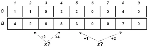
Fig. 6. Illustration of two queries in the Bh−CBF with the Bh=2
sequence D = {1,2,4}. The jth selected hash entry includes a pair of
counters: cj with fixed increments, andaj with variable increments. The kvariable increments of each element are presented. For each element, we consider the exact values of both counters ink= 2hash entries to calculate the membership probability based on theBh−CBF.
and
γ= Pr (Q=q|X= 0) =
( ∏k
j=1,I(j)=0
Pr (Cj=cj|X= 0) )
·
( ∏k
j=1,I(j)=1
Pr (Yj=yj|X= 0) )
=
( ∏k
j=1,I(j)=0
(n
cj
)(k
m
)cj(
1− k m
)n−cj)
·
( ∏k
j=1,I(j)=1
(n
yj
)( k
m·ℓ
)yj(
1− k m·ℓ
)n−yj)
.
Finally, we have that
Pr (x∈S|Bh−CBF) = β·Pr (X= 1) β·Pr (X= 1) +γ·Pr (X= 0)
= Pr (X= 1)
Pr (X= 1) +∏kj=1,I(j)=0mn··ck
j ·
∏k
j=1,I(j)=1
n·k
m·ℓ·yj ·Pr (X= 0)
= m
k·δ·Pr (X= 1)
mk·δ·Pr (X= 1) + (n·k)k·Pr (X= 0)
for δas defined above.
We would like now to demonstrate the similarity of the formulas of Pr (x∈S|CBF) and Pr (x∈S|Bh−CBF)
as presented in Theorem 2 and Theorem 5, respec-tively. Simply, Pr (x∈S|CBF) can be obtained from
Pr (x∈S|Bh−CBF) by setting I(j) = 0 for j ∈
{1, . . . , k}, which yields that δ=∏kj=1cj. The intuition for
that is as follows. In the CBF, the value ofδin the formula of
Pr (x∈S|CBF)equals the product of the number of inserted elements to each of the k hash entries used by the element x. In the Bh−CBF we can obtain, for some of the hash
entries used by x, not only the value of cj which represents
the number of inserted elements into the jth hash entry, but
alsoyj, the number of inserted elements with the same variable
increment as the element x. For such counters, the value of the counter cj is replaced in the formula of δ by a more
informative value which is ℓ·yj, where ℓ is the number of
possible variable increments. Of course, we should try to avoid the influence of elements inserted into this hash entry with other variable increments that are guaranteed not to be the element xitself. Unfortunately, ifcj > h, we cannot do that
As in the CBF, for each value of α we can consider the membership probabilityPr (x∈S|Bh−CBF)based on the Bh−CBF, in order to decide on the optimal answer to a
membership query. Again, in some cases it might be better to return a negative answer even if Pr (x∈S|Bh−CBF)>0
and the indication of the Bh−CBF is positive.
Example 2: Figure 6 illustrates queries of two elementsx and z in a Bh−CBF with the set of variable increments D = {1,2,4}. We can see all the 6 sums 2 elements of D are distinct: 1 + 1 = 2,1 + 2 = 3,1 + 4 = 5,2 + 2 = 4,2 + 4 = 6,4 + 4 = 8. Therefore, D is a Bh=2
sequence. For the element x, since c1 = 1, c2 = 2 ≤ h
we can determine the multiplicities y1 = 1, y2 = 2 of the
variable increments vg1(x) = 2, vg2(x) = 4 in the sums
a1 = 2, a2 = 8, respectively. By Theorem 5, we have that Pr (x∈S|Bh−CBF) =
mk·δ·Pr(x∈S)
mk·δ·Pr(x∈S)+(n·k)k·(1−Pr(x∈S))
for δ = (ℓ·y1)·(ℓ·y2) = (3·1)·(3·2) = 18. Likewise,
for the element z,c1 = 2, a1= 3, vg1(z)= 1 and necessarily
y1= 1. However, sincec2= 4> h, we cannot determine the
multiplicity ofvg2(z)= 2in the suma2= 7 = 1 + 1 + 1 + 4 =
1 + 2 + 2 + 2. Thus,I(2) = 0and theBh−CBF-based
mem-bership probability takes into accountc2and noty2. Therefore, Pr (z∈S|Bh−CBF) =
mk·δ·Pr(z∈S)
mk·δ·Pr(z∈S)+(n·k)k·(1−Pr(z∈S)) for
δ= (ℓ·y1)·(c2) = (3·1)·4 = 12.
VII. DISTRIBUTED-CACHEAPPLICATION
Eliminating the Bloom paradox and the ability to calculate the membership probability based on the exact values of the CBF counters can improve the performance of many applications. In this section, we suggest an example for such an application.
A. Model
Our model is based on the model of cache sharing among Web proxies as described in the seminal paper presenting the CBFs [2]. In theSummary Cachesharing protocol suggested in this paper, each proxy keeps an array of CBFs that summarize the cache content of each of the other proxies. If a proxy encounters a local cache miss, it examines the summaries of the contents of the other caches. It then sends a query message only to the proxies with a positive membership indication for the existence of the required data element in their caches, based on the corresponding CBFs. Since CBFs have no false negatives, only this subset of the proxies might contain this specific data element. Since the content of each of the caches dynamically changes and deletions have to be supported, we cannot simply use Bloom filters in this case, and need to keep counters. In their model, the performance is measured by the total amount of network traffic as a function of the memory size dedicated for the summaries.
[image:9.612.316.558.52.133.2]Based on the theory we presented, it is possible to consider the exact values of the CBF counters in order to calculate the membership probability in each of the possible proxies. Thus, we can further distinguish between the proxies with a positive indication. For instance, we can prefer to probe first the proxies with higher chances to have the element in their caches.
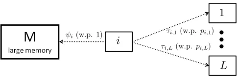
Fig. 7. Illustration of the cache sharing model. A query of an elementx can be sent from proxy i toL−1other proxies. A query sent to proxy j ∈ ({1, . . . , L} \ {i}) has a traffic cost of τi,j and is successful w.p. pi,j= Pr (x∈Sj|CBFi,j). Alternatively, the elementxcan be found with certainty in a single larger memory with a relatively expensive traffic costψi.
As illustrated in Figure 7, we generalize the model as follows. Let Lbe the number of proxies and letSi represent
the content of cache i for i ∈ {1, . . . , L}. The set of all possible data elements is denoted by U. We assume that different proxies may have different traffic costs for a query they send to each of the other proxies. Let τi,j > 0 denote
the traffic cost of a query sent from proxy i to proxy j for i, j∈ {1, . . . , L}.
We also assume that the a priori probability Pr(x ∈ Si)
for the membership of each data element x ∈ U in each of the caches is available. The probabilities may be uniform or non-uniform overU and may vary in each of the caches. For the required data element x∈U, we denote by pi,j the
membership probability based on the CBF held by proxyifor summarizing the cache content of proxyj. These probabilities are assumed independent. By denoting this CBF byCBFi,j,
we have pi,j= Pr (x∈Sj|CBFi,j).
Last, we assume that all of the elements can be found in a special proxy (denoted by the index L+ 1) with a large memory containing all the elements in U. A query sent to this special proxy from each other proxy i has a relatively expensive traffic costψi. We also refer to the otherLproxies
as regular proxies.
B. Optimal Query Policy
Given a request for a data element in one of the proxies, we would like to determine the order of the queries it should send in order to minimize the total expected cost of queries until the element is found. Of course, we can clearly see, as suggested also in [2], that since all the queries costs are positive there is no reason to send a query to a proxy when the CBF indicates that it does not contain the required element. In addition, we observe that in this model, any two queries should not be sent in parallel. By sending these queries one after another, the expected cost is reduced since if the first is successful, then the second query can be avoided.
When proxyiencounters a local cache miss for the query of an elementx∈U, it should consider the success probability of probing a proxyj that satisfiespi,j= Pr (x∈Sj|CBFi,j)>
0. It should also take into account the cost of a single query to each of these proxiesτi,j and the traffic cost to the special
proxy with all the data elementsψi.
scenarios can be described as a special case of a very general problem described in [35].
General case: In the first scenario, we deal with general
traffic costs and just assume that each of the costs τi,j are
positive without any additional constraints.
The next theorem presents the optimal order of queries for minimizing the expected cost. Intuitively, we want to access first proxies with high success probability. We also prefer proxies with low query cost. The theorem shows that we should compare the ratio of these two parameters for each of the proxies and query them in a non-increasing order of the ratios. After encountering some failures while accessing the proxies with high ratio, we are left only with proxies that have a relatively low ratio, i.e. proxies with low success probability or high traffic cost. At some point, we prefer to access the special proxy despite its high cost, and obtain the data element with certainty rather than probing the proxies left.
As mentioned earlier, the theorem follows from a more general claim presented in [35] in a different context. We present the shorter and easier proof of this special case.
Theorem 6: An optimal sequence of queries performed by proxy i that minimizes the expected total cost is given by accessing the proxies (the regular proxies or the single special proxy) in a non-increasing order of the ratio of their success probability and the query cost, i.e. the ratio pi,j
τi,j for a proxy
j ∈({1, . . . , L} \ {i})or ψ1
i for the special proxy.
Indeed, after accessing a proxy with a success probability of 1 (and in particular the special proxy), the order of the next queries can be arbitrary.
Proof: The proof is by contradiction. We show that for any sequence with different order, we can switch the order of two queries and reduce the expected cost. For the sake of simplicity, we also use the notationspi,L+1andτi,L+1for the
success probability (which equals 1) and the query traffic cost (denoted earlier also byψi) of the special proxy, respectively.
Clearly, after accessing a proxy with a success probability of 1, the data element is available, any additional queries are always useless. Letσ= (σ1, . . . , σL)be an optimal order such
thatσj ∈({1, . . . ,(L+1)}\{i})and for each1≤j < t≤L,
we have σj ̸= σt. We denote by σℓ the first proxy in this
order that has a success probability of 1. Then, pi,σℓ = 1and
pi,σj <1 for j ∈ {1, . . . ,(ℓ−1)}. The special proxy is an
example for such a proxy and thus there is always at least one proxy with this property. LetE(σ)be the expected traffic cost when the orderσ is used.
If σ does not satisfy the presented condition, there are two adjacent indices 1 ≤ k, k + 1 ≤ ℓ such that
pi,σk τi,σk <
pi,σk+1
τi,σk+1. We then consider a second order σ′ =
(σ1, . . . , σk−1, σk+1, σk, σk+2, . . . , σL) obtained by flipping
the order of the kth and (k+ 1)th queries in σ. We show that E(σ′)<E(σ), a contradiction to the optimality ofσ.
Clearly, sinceσandσ′ differ only in the two indiceskand k+ 1, such a change can influence the total traffic cost only when the firstk−1queries fail and at least one of these two queries succeeds. Assuming that the first k−1 queries fail (it happens w.p. pf ail =
( ∏k−1
j=1(1−pi,σj) )
), and both of these two considered queries succeed (w.p.pi,σk·pi,σk+1), the
change in the traffic cost isτi,σk+1−τi,σk with the switching
from σ to σ′. This is because the kth and last query is now
sent to proxyσk+1 instead of toσk. Likewise, when only the
query sent toσksucceeds, the cost is increased byτi,σk+1with
the order change. Last, if only σk+1 has the data element,
the cost is decreased by τi,σk. To summarize, we have that
E(σ′)−E(σ) = pf ail·
(
pi,σk ·pi,σk+1 ·(τi,σk+1−τi,σk) +
pi,σk·(1−pi,σk+1)·τi,σk+1−(1−pi,σk)·pi,σk+1·τi,σk )
=
pf ail·
(
pi,σk·τi,σk+1−pi,σk+1·τi,σk )
<0. A contradiction to the optimality of E(σ).
Simple case: We now consider the simple case in which
each proxyihas the same traffic costτito each of the regular
proxies such thatτi=τi,j forj ∈({1, . . . , L} \ {i}).
The next theorem presents the optimal order of queries for a minimal expected cost. Now, since the query costs are fixed, we access the proxies in a decreasing order of their success probability and again prefer to access the special proxy after some failures rather than examining the other left proxies with low success probability.
Theorem 7: An optimal sequence of queries performed by proxy i that minimizes the expected total cost is given by accessing the proxies in a non-increasing order of their success probability. When the left proxies have a success probability smaller than τi
ψi, the next and last query should be sent to the
special proxy.
Proof:The proof directly follows from Theorem 6 based on the following observations. Clearly, if the query cost to each of the other proxies is fixed then a non-increasing order of the success probability is also a non-increasing order of the ratio of the success probability and the query cost. Likewise, if (∀j∈({1, . . . , L} \ {i})),τi=τi,j, thenpi,j< ψτii exactly
when pi,j
τi,j < 1
ψi and the next query should be sent to the
special proxy.
It is interesting to see that the last result can be useful even in some cases where the values of the a priori membership probabilities are not available. With the assumption of fixed query costs, if we further assume that thea priorimembership probability of an element is identical among the different proxies, we can prefer one regular proxy on another. Based on Theorem 2, the order can be determined based only on the values of the product of thekcounters in the correspond-ing CBFs, without knowcorrespond-ing the exact values of the success probabilities in each proxy.
VIII. SIMULATIONS
A. Bloom Filter Simulations
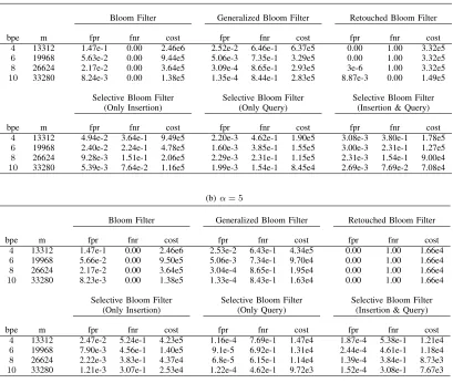
Table II compares the false positive rate (fpr), false negative rate (fnr) and the total cost for the Bloom Filter (BF) [1], Generalized Bloom Filter (GBF) [20], Retouched Bloom Filter (RBF) [19] and the suggested Selective Bloom Filter with its three variants.
We assume a set S composed of 256 elements from each of 13 types of elements, such that n = |S| = 28 ·13 = 256·13 = 3328. Each subset of 256 elements is selected homogeneously among sets of sizes211,212, ...,223. Thus, for
prioriset-membership probability of2−(i+2) andN=|U|=
∑13
i=12
i+10 = 16775168. The numbers of bits per element
(bpe) are 4,6,8 and10 such thatm=n·bpe.
As usual, the false positive rate (fpr) is calculated among the N−nelements ofU\S and the false negative rate (fnr) is calculated among thenmembers ofS. In the calculation of the total cost, we assume that WF P = 1 andWF N =αsuch
that the cost equals(N−n)·fpr +n· fnr·α. The results are presented for the valuesα= 100 andα= 5, which illustrate two possible scenarios for the ratio of the two error costs. In the Bloom Filter and in the three variants of the Selective Bloom Filter we usek≈ln(2)·(m/n)hash functions. In the Generalized Bloom Filter we use k1 = k hash functions to
select bits to be set. Likewise, the number of functions used to select bits to reset, k0 ∈[1, k1−1], was chosen such that
the total cost is minimized. For the Retouched Bloom Filter we used theRatio Selectionas the clearing mechanism. In this heuristic, shown to be the best scheme in [19], the bits to be reset are selected, such that the ratio of the additional false negatives and the cleared false positives is minimized.
We first note that when thea prioriset-membership proba-bilities are available in the insertion process as well as in the query process, the Selective Bloom Filter always improves the total cost achieved in BF, GBF and RBF, even whenα= 100
and accordingly the cost of a false negative is very high. For instance, when the probabilities are used in the insertion as well as in the query, with a memory of 4 bits per element (and α = 100) the total cost is 1.78e5 in comparison with 2.46e6, 6.37e5 and 3.32e5 in BF, GBF and RBF respectively, i.e. a relative reduction of 92.76%, 72.04%, 46.46%.
If α = 5, the cost of a false negative is relatively small. As a result, optimizing the tradeoff of fpr vs. fnr results in an (fpr,fnr) pair of (1.87e-4, 5.38e-1) instead of (3.08e-3, 3.80e-1) forα= 100. That is, as expected, the fpr is smaller and the fnr is larger when the relative cost of fnr is smaller. Ifα= 5, the cost is 1.21e4 instead of 2.46e6 in BF. This is a significant improvement by more than two orders of magnitude.
We can also see that, in this simulation, the contribution of the a prioriprobabilities is more significant in the query process than in the insertion process. For instance, with 4 bits per element andα= 100, the cost is 9.49e5 if the probabilities are used only in the insertion, while it is only 1.90e5 when they are used only during the query. It can be explained by the fact that in our experiment, the set U\S is much larger than the setS itself. Thus, the effect of avoiding the false positives of elements with smaller a prioriset-membership probability during the query is larger than the effect achieved by avoiding the insertion of elements with such probabilities.
B. Counting Bloom Filter Simulations
In this section we conduct experiments on CBFs. We first examine the CBF-based membership probability in compari-son with Theorem 2.
Then, we try to use these probabilities to further reduce the expected cost of a query.
The setS is defined exactly as in the previous simulation. It again includesn= 13·256 = 3328elements of13types with
0 20 40 60 80 100
0 0.2 0.4 0.6 0.8 1
membership probability
counters product
[image:11.612.312.576.245.336.2]P = 2−3 (theory) P = 2−3 (simulation) P = 2−5 (theory) P = 2−5 (simulation) P = 2−7 (theory) P = 2−7 (simulation)
Fig. 8. CBF-based membership probability for elements witha priori set-membership probabilityP = Pr(x∈S). The probability is based onk=6 counter valuesand compared with Theorem 2.
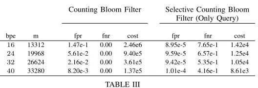
Counting Bloom Filter Selective Counting Bloom Filter (Only Query)
bpe m fpr fnr cost fpr fnr cost
16 13312 1.47e-1 0.00 2.46e6 8.95e-5 7.65e-1 1.42e4 24 19968 5.61e-2 0.00 9.40e5 9.59e-5 6.57e-1 1.25e4 32 26624 2.16e-2 0.00 3.61e5 9.42e-5 5.35e-1 1.05e4 40 33280 8.20e-3 0.00 1.37e5 1.01e-4 4.16e-1 8.61e3
TABLE III
SIMULATION RESULTS FORCOUNTINGBLOOMFILTERS WITHα= 5. SIMULATION PARAMETERS ARE THE SAME AS INTABLEII.
a prioriprobabilities of 2−3,2−4, ...,2−15. Here, since CBFs
with four bits per entry are used, we consider bpe values of
16,24,32and40.
Figure 8 displays the membership probability based on the values of the k = 6 counters. According to Theorem 2, the probability can be described as a function of the product of these k counters. The figure presents the results for up to a product of 100, since larger products were encountered in the simulations with a negligible probability. The simulated probabilities for the most common values are compared with the theory. The dependency in the a priori set-membership probability is demonstrated again. For instance, if the product is 8, the observed probabilities are 0.90594,0.68504 and
0.34679for thea prioriprobabilities2−3,2−5,2−7. Likewise,
to obtain a membership probability of at least0.8, the minimal required products are5,23and91, respectively.
(a)α= 100
Bloom Filter Generalized Bloom Filter Retouched Bloom Filter
bpe m fpr fnr cost fpr fnr cost fpr fnr cost
4 13312 1.47e-1 0.00 2.46e6 2.52e-2 6.46e-1 6.37e5 0.00 1.00 3.32e5 6 19968 5.63e-2 0.00 9.44e5 5.06e-3 7.35e-1 3.29e5 0.00 1.00 3.32e5 8 26624 2.17e-2 0.00 3.64e5 3.09e-4 8.65e-1 2.93e5 3e-6 1.00 3.32e5 10 33280 8.24e-3 0.00 1.38e5 1.35e-4 8.44e-1 2.83e5 8.87e-3 0.00 1.49e5
Selective Bloom Filter Selective Bloom Filter Selective Bloom Filter (Only Insertion) (Only Query) (Insertion & Query)
bpe m fpr fnr cost fpr fnr cost fpr fnr cost
4 13312 4.94e-2 3.64e-1 9.49e5 2.20e-3 4.62e-1 1.90e5 3.08e-3 3.80e-1 1.78e5 6 19968 2.40e-2 2.24e-1 4.78e5 1.60e-3 3.85e-1 1.55e5 3.00e-3 2.31e-1 1.27e5 8 26624 9.28e-3 1.51e-1 2.06e5 2.29e-3 2.31e-1 1.15e5 2.31e-3 1.54e-1 9.00e4 10 33280 5.39e-3 7.64e-2 1.16e5 1.99e-3 1.54e-1 8.45e4 2.69e-3 7.69e-2 7.08e4
(b)α= 5
Bloom Filter Generalized Bloom Filter Retouched Bloom Filter
bpe m fpr fnr cost fpr fnr cost fpr fnr cost
4 13312 1.47e-1 0.00 2.46e6 2.53e-2 6.43e-1 4.34e5 0.00 1.00 1.66e4 6 19968 5.66e-2 0.00 9.50e5 5.06e-3 7.34e-1 9.70e4 0.00 1.00 1.66e4 8 26624 2.17e-2 0.00 3.64e5 3.04e-4 8.65e-1 1.95e4 0.00 1.00 1.66e4 10 33280 8.23e-3 0.00 1.38e5 1.33e-4 8.43e-1 1.63e4 0.00 1.00 1.66e4
Selective Bloom Filter Selective Bloom Filter Selective Bloom Filter (Only Insertion) (Only Query) (Insertion & Query)
bpe m fpr fnr cost fpr fnr cost fpr fnr cost
[image:12.612.102.511.60.406.2]4 13312 2.47e-2 5.24e-1 4.23e5 1.16e-4 7.69e-1 1.47e4 1.87e-4 5.38e-1 1.21e4 6 19968 7.90e-3 4.56e-1 1.40e5 9.1e-5 6.92e-1 1.31e4 2.44e-4 4.61e-1 1.18e4 8 26624 2.22e-3 3.83e-1 4.37e4 6.8e-5 6.15e-1 1.14e4 1.39e-4 3.84e-1 8.73e3 10 33280 1.21e-3 3.07e-1 2.53e4 1.22e-4 4.62e-1 9.72e3 1.52e-4 3.08e-1 7.67e3
TABLE II
COMPARISON OF FALSE POSITIVE RATE(FPR),FALSE NEGATIVE RATE(FNR)AND THE TOTAL COST FORBLOOMFILTER, GENERALIZEDBLOOMFILTER, RETOUCHEDBLOOMFILTER AND THE SUGGESTEDSELECTIVEBLOOMFILTER WITH THREE VARIANTS. IN THE FIRST,THEa prioriSET-MEMBERSHIP PROBABILITY IS USED ONLY DURING THE INSERTION OF THE ELEMENTS,WHILE IN THE SECOND VARIANT IT IS USED ONLY IN THE QUERY PROCESS AND IN THE THIRD ONE IT IS USED IN BOTH OF THEM. THE TOTAL NUMBER OF INSERTED ELEMENTS ISn= 256·13 = 3328WITHa prioriSET-MEMBERSHIP
PROBABILITIES OF2−3,2−4, ...,2−15AND|U|= 16775168.
see an additional improvement of up to 11.43%. This reduction in the total cost is due to the more accurate calculation of the membership probability based on the information on the exact values of the counters. Such information is not available in the Selective Bloom Filter.
C. Trace-Driven Simulations
We now want to explore the tradeoff of the false positive rate and the false negative rate in the Selective CBF. To do so, we conduct experiments using real-life traces recorded on a single direction of an OC192 backbone link [36]. We used a 64-bit mix hash function [37] to implement the requested hash functions. The hash functions are calculated based on the 5-tuple (Source IP, Destination IP, Source Port, Destination Port, Protocol).
The Selective CBF represents here, using 30 bits per el-ement and 4 bits per counter, a set of n = 210 different tuples that we encounter in a short period of 3614 µs. Our queries are based on N = 220 tuples (that includes the
first n) that were encountered later on during a longer time
interval. This yields ana prioriset-membership probability of n/N= 210/220= 2−10.
Figure 9(a) illustrates this tradeoff. The three dashed lines draw the tradeoff achieved using the Selective CBF with the k= 4,5and6hash functions. Three points are located on the y-axis. They present, of course, the typical false positive rate of the CBF where no false negatives are allowed. The rates are0.03086,0.02850,0.02908, respectively and the minimum is achieved fork= 5≈30/4·log(2). Thus, ifWF N is large
enough andα→ ∞, the optimal number of hash functions is k= 5.
We earlier showed that the membership probability is an increasing function of the product of thek counters. In each of these three lines, each point illustrates a different threshold of the counters product such that a negative answer is returned only if the product is smaller than the threshold. As explained in Section V, in order to minimize the expected cost, each value ofαcan be translated to a probability threshold of α1+1 by Theorem 4 and later on also to a product threshold. For instance, forα= 2.4, the probability threshold is α+11 = 10
34.