1 1
2 3 4
Characterizing Uncertainty and Learning in the Economics of Resource and Environmental Management 5
6
Authors: Jacob LaRiviere (Tennessee & Microsoft), David Kling (Oregon State), James N. Sanchirico (UC 7
Davis), Charles Sims (Tennessee), Michael Springborn (UC Davis) 8
9 10
JEL codes: Q2, Q5, Q3, D83 11
Keywords: Optimal Control, Updating, Option Value 12
Abstract: Environmental and resource economists use models that often include at least one of several 13
broad classes of uncertainty and at least one of several different ways to reduce uncertainty through 14
learning. In this paper we delineate several different forms of uncertainty, stochasticity, and learning in 15
a standard environmental and resource economics framework. We then use that framework in 16
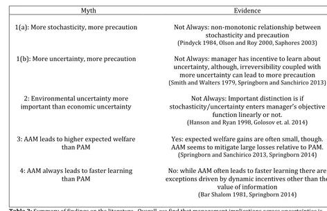
surveying the literature to find if there is support for four different “myths” associated with uncertainty 17
and learning in environmental management. We find that these management myths are often not 18
generally true across different forms of stochasticity, uncertainty and learning. 19
2
Uncertainty permeates the economics of natural resource and environmental management. Some well-29
known examples are uncertain damages from pollution, asymmetric information regarding firms’ 30
abatement costs, stochastic resource growth, imperfectly observed resource stock levels, and 31
uncertainty regarding the correct structure of resource growth or pollution decay. Given that 32
uncertainty is a significant aspect of most policy-relevant environmental and resource management 33
problems, two important questions for researchers are: (1) what types of uncertainty are relevant for 34
my problem; and (2) how portable are insights from studying one type of uncertainty to another 35
situation? 36
The contemporary resource and environmental management literature models several broad classes of 37
uncertainty, several different ways to reduce uncertainty through learning, and several different 38
solution methods. To help researchers navigate the extensive and sometimes confusing literature, we 39
pursue two goals in this paper. First, we define several forms of uncertainty, stochasticity, and optimal 40
information acquisition in environmental and resource economics using the decomposition approach of 41
Walters and Hilborn (1976) and Charles (1998).1 We pay particular attention to the optimal way to learn 42
about and manage environmental and natural resources in the presence of uncertainty that can be 43
reduced through learning. In the following section of the paper we incorporate each type of uncertainty 44
and learning into a unified framework. Specifically, we concentrate on the canonical perspective of a 45
social planner seeking to maximize the expected net present value of a generic environmental or 46
resource stock. This simple model may be extended to capture common second-best problems (e.g., 47
profit maximization subject to minimum extinction risk or maximum allowable pollution levels) and 48
spans both environmental and resource management contexts. 49
3
Second, we use the model and framework to address “myths” associated with uncertainty and learning. 50
The four myths we consider are: (1) greater levels of uncertainty result in more precautionary 51
management (e.g., Gollier et al. 2000); (2) reductions in environmental uncertainty have greater value 52
than reductions in economic uncertainty (e.g., Sethi et al. 2005); (3) management strategies with active 53
learning about an economic or ecological system lead to substantially higher welfare than those with 54
passive learning (e.g. Bond & Loomis 2009); and (4) managers who try to actively learn do so faster than 55
those who passively learn (e.g. Springborn & Sanchirico 2013). Evaluating these myths is the primary 56
contribution of the paper. Importantly, we show that each myth can manifest in different ways in 57
different environment and resource problems. As a result, general conclusions about uncertainty and 58
learning are limited because the literature’s results are often context-dependent. 59
In what follows, we introduce a basic framework, which provides structure for our subsequent 60
discussion. We then evaluate each myth and highlighting where it is and is not true. We conclude with a 61
summary and list some potential opportunities for further research. For a more complete treatment of 62
risk for policy, we refer readers to Morgan and Henrion (1990) and Pindyck (2007). 63
64
Stochasticity, Uncertainty and Learning 65
Most resource or environmental management problems involve multiple types of uncertainty. Due to 66
space limitations we focus on models grounded in subjective expected utility theory (SEU), by far the 67
dominant analytical framework in economics and allied quantitative disciplines (Gilboa 2009). To 68
anchor our discussion and distinguish among different types of uncertainty, we introduce a simple “toy” 69
model of a management problem. Modeling a single decision maker is the traditional first step in 70
developing intuition for dynamic environmental and resource economic problems (Clark 1990). We 71
4
The goal of the manager is to maximize the expected net present value (NPV) of a stream of rewards 73
(πt). Examples include the discounted flow of rents from resource extraction (e.g., a fishery or mine) or 74
discounted flow of net benefits of pollution abatement. We will couch much of the discussion below in 75
the context of two classic management problems from the resource and environmental literature: 1) 76
maximize the discounted flow of profits from a stock of fish, and 2) minimize the discounted flow of 77
damages and control costs from a stock (ambient concentration) of pollution like SO2. 78
In the model, the manager decides in each period (t) how much to manipulate a physical state variable 79
(xt) by selecting the value of a control variable (ut). In the case of a fishery, a control variable could be 80
total harvest in a period and the state variable is the stock of fish. For the pollution management 81
problem, a control variable could be pollution emissions in a period and the state variable is the stock of 82
the pollutant. Formally, the manager’s problem is: 83
max
{𝑢𝑡}
𝐸 [∑∞𝑡=0𝛿𝑡𝜋(𝑥𝑡, 𝑢𝑡, 𝜖𝑡𝜋; Θ𝑡𝜋)] (1) 84
subject to: 𝑥𝑡+1= 𝑓(𝑥𝑡, 𝑢𝑡, 𝜖𝑡 𝑓
; Θ𝑡𝑓),
85
where 𝝐𝑡 = (𝜖𝑡𝜋, 𝜖𝑡 𝑓
) is a vector of stochastic terms which operate on the objective function (e.g., 86
stochastic output prices) or the state equation (e.g., stochastic shocks to the resource stock). 𝚯𝑡 = 87
(Θ𝑡𝜋, Θ𝑡 𝑓
) is a set of economic and biophysical parameters. Along with the state and control variables, 88
the within-period reward π( ) is a function of the economic shocks and parameters. 89
The function f(), known as the state equation, determines the evolution of the state variable. The 90
transition of the state to the next period is a function of the current state and control variables. We 91
assume that the next period’s state is also a function of stochastic shocks (𝜖𝑡𝑓)and parameters (Θ𝑡𝑓). For 92
a fish harvest problem, these parameters include the natural environment’s carrying capacity and 93
5
include the pollutant’s decay rate. The structure of the state equation encodes the physical relationship 95
between the state and control variables, meaning it must be at least partially understood in order for 96
the manager to predict the consequence of an action. In general the state equation is often nonlinear or 97
features spatial or multi-state structure that adds considerable complexity to the manager’s problem. 98
Different Forms of Uncertainty 99
This article considers four kinds of “uncertainty” that may be present in the management problem and 100
which receive significant attention in the literature: stochasticity, parametric uncertainty, model 101
uncertainty and state uncertainty. Indeed, it may be the case that all four types of uncertainty are 102
simultaneously present. 103
Stochasticity 104
Natural resource and environmental management often deals with dynamic processes influenced by 105
stochasticity, often described as intrinsic variability, shocks, or “noise”. In our toy model, stochasticity is 106
represented by the random vector 𝝐𝑡. Both within-period outcomes (e.g. rewards) and state dynamics 107
can be stochastic. For example, 𝝐𝑡 can enter both the rewards function π( ) and the state equation f() 108
either additively or multiplicatively.2 Stochastic terms are typically drawn from a known distribution 109
(Reed 1979), specified here by parameters in 𝚯𝑡.3 The appropriate distributional assumption the 110
stochastic component are often context dependent. For example a lognormal distribution may be 111
appropriate if stochasticity is more appropriately modeled multiplicatively. 112
2 In different and more complicated models, such as multiple decision makers engaging in a game, economic stochasticity can compound and arriving at a market equilibrium can itself become challenging. We ignore these issues and only consider bounded economic stochasticity in this paper.
6
Even within a short time scale, it is rarely technically feasible (much less cost-effective) to perfectly 113
forecast state variables. Sources of natural variability (e.g. ocean upwelling anomalies, droughts, etc.) 114
are difficult to predict. There are also a variety of sources of economic variability, for example resource 115
commodity prices (Pindyck 1984). In order to capture natural and economic variability and account for 116
the challenge of prediction, modelers often introduce stochasticity. 117
An important but subtle point with respect to how stochasticity is modeled is that even though it is 118
irreducible (i.e. cannot be ameliorated through learning), it is measurable in that its distribution may be 119
specified precisely. This characteristic implies that in any resource or environmental model: 1) the 120
manager knows all functions and distributions of stochastic variables; and 2) these functional 121
relationships perfectly predict the dynamics of the management problem conditional on stochastic 122
elements. 123
However, managers still have an incentive to obtain new information in stochastic models. As noted by 124
Pindyck (2007), the concept of option value (Arrow and Fisher 1974; Dixit and Pindyck 1994) establishes 125
that merely accounting for new information about the outcome of an uncertain stochastic shock tends 126
to increase the value of delaying an irreversible action.4 Irreversibility may represent the minimum 127
viable population of a renewable resource below which the resource goes extinct. In equation (1), 128
irreversibility could be modeled by including an absorbing barrier 𝑥̅ into the state dynamics, such that 129
changes in the state variable are terminated once 𝑥𝑡 crosses 𝑥̅ (e.g., 𝑥̅ is the minimum viable 130
population). Alternatively, irreversibility may result from limiting the frequency of adjustments to the 131
control variable due to sunk costs (Pindyck 2000) or institutional failures that limit available 132
7
management choices (Arrow et al. 2000). This irreversibility constrains future adjustments to the 133
management action in response to new information (e.g., resolution of stochasticity). The inability to 134
adjust management to new information is costly and hence information is valuable. When management 135
actions today limit the manager’s future action space there is an opportunity cost of irreversible 136
deviations from the status quo through forgone information value or the forfeiture of the option to react 137
to future realizations of the random variable (Conrad 1980). In a sense, then, the option value is the 138
value of having a less restrictive control space – a value of flexibility in the face of an uncertain future. 139
140 141
Parametric Uncertainty 142
Above we assumed that while the system is stochastic but that that manager knows the characteristics 143
of the system perfectly (e.g., the manager knows 𝚯𝑡 with certainty). Under parametric uncertainty, the 144
manager plans without precisely knowing one or more components of the system (e.g., one parameter 145
of 𝚯𝑡 is unknown). For example, a fishery manager may specify regulations like a catch limits for a stock 146
without knowing its growth rate precisely (Springborn 2014). An environmental manager may be 147
uncertain about the origin of a non-point source pollutant or pollution transfer coefficients more 148
generally (Fowlie and Mueller 2013 and Carson and LaRiviere 2015). In the fisheries example, the 149
manager could believe the intrinsic growth rate of a species could be either high, medium or low with 150
different discrete probabilities. Alternatively, uncertainty over growth could vary continuously, e.g. 151
according to a normal distribution. In contrast to stochasticity, parametric uncertainty (along with state 152
and model uncertainty) is reducible through learning, at least conceptually. However, if such learning is 153
8
case, parametric uncertainty could lead to a less “predictable” system when added to a purely stochastic 155
state equation. 156
157
Model Uncertainty 158
Model uncertainty differs from parametric uncertainty in that the manager does not precisely know the 159
true functional forms of one or more of the model’s equations. In a fisheries context there could be 160
uncertainty over whether the Ricker or Beverton-Holt recruitment function is most appropriate. In the 161
context of managing waterfowl harvest, for over a decade the U.S. Fish and Wildlife service has used a 162
framework that admits multiple competing models of population dynamics and harvest effects 163
(Johnson, 2011). In the air quality example it could be linear, quadratic or exponential decay rates. 164
Particularly if the manager cares about predicting out of sample, as in the case of climate change and 165
GHG levels, knowing the correct model can be very valuable. In equation (1), the manager might be 166
uncertain about which of two different equations, f1() versus f2(), governs the evolution of the state 167
variable. Allowing multiple models generalizes the manager’s problem; for example, the state equation 168
could become a weighted average on the various competing models. 169
170
State Uncertainty 171
State uncertainty arises when a physical state variable is observed imperfectly (e.g., when the manager 172
in equation (1) does not know the precise value of xt).5 This typically occurs when the true state is 173
difficult to observe (e.g. wild species populations or pollution conditions over space) and assessments 174
9
are imperfect (e.g. when estimating fish stocks or observing coarse air quality data). For example, even 175
though there are air pollution monitors throughout many countries, they only take readings at discrete 176
locations leading to uncertainty about ambient pollution levels between monitoring stations. 177
State uncertainty is conceptually distinct from parameter and model uncertainty for the following 178
reason: the latter two typically involve uncertainty about a fixed object (e.g. a true parameter value) 179
while state uncertainty centers on an unknown value that is changing over time at least in part due to 180
management choices. Furthermore, with parameter uncertainty, any prediction errors in the stock 181
dynamics by the manager do not compound over time since the manager observes this state variable 182
perfectly at some point in each period. 183
184
Learning 185
The general topic of learning is a broad and important question in economics with a long history in the 186
literature (Blackwell 1951 and Marschak and Miyasawa 1968). Economic models of learning typically 187
feature a Bayesian updater who can endogenously acquire noisy signals about an uncertain feature of 188
the decision making environment (Rothschild 1974, Sims 2003, Milani 2007, Schwartzstein 2014, and 189
Caplin and Dean 2015). In a resource and environmental management context, parameter, model, and 190
state uncertainty can often be reduced over time through learning. The traditional approach to 191
modeling learning is to introduce a parameterized distribution characterizing the manager’s beliefs over 192
the true level or form of an uncertain model component. For example, a beta distribution might capture 193
uncertainty over the true value of a process governing an air pollution dissipation.6 194
10
Formally, let the parameters of the distribution summarizing the state of beliefs in a period be 195
given by 𝛃𝑡. Let information dynamics be given by: 196
𝛃𝑡+1= 𝑔(𝛃𝑡). 197
The function g() captures how the manager changes their beliefs about a system over time. Beliefs 198
usually are assumed to be a Bayesian update performed using observed state or state measurement 199
dynamics in response to the level of control. 7 For example, an environmental manager may learn from 200
observing how reductions in emissions affect ambient pollution levels.8 Since state variables are 201
inherently dynamic (whereas parameters and model of the state equation are fixed) updating beliefs 202
about an unknown state must account for both stochastic state dynamics and learning about the level of 203
an uncertain state variable at a given point in time.9 The updating process usually is modelled 204
iteratively after a period’s stochastic outcomes are observed and before the manager makes the next 205
period’s decisions. 206
207
Different Management Styles to Learning about Uncertainty 208
This section describes how the manager’s problem changes given the modeler’s assumptions on how 209
learning occurs. Learning is operationalized by how the modeler chooses to let the timing of belief 210
7 Uncertainty may also be reduced by investing in direct learning. For example, the manager can monitor to reduce stock uncertainty. In the fisheries case, in contrast to making inferences about the stock from effort-catch observations, the manager could pay for stock assessments. Similarly, the manager could hire additional ecologists to refine parametric uncertainty.
8 Learning problems typically involve an assumption that the true level or form of the imperfectly understood model component is fixed, i.e. not dynamic. For example, a climate policy model might allow for the parameter describing climate forcing to be unknown, but the true level is assumed to be constant. While this is sometimes a strong assumption it serves to simplify the information dynamics.
11
updating to be incorporated or ignored at two points in the manager’s problem: 1) solving for the 211
optimal policy and 2) stepping forward in time.10 First, when solving for the optimal policy, the manager 212
can recognize the implications of learning and choose the control in a way that is sensitive to the value 213
of what can be gleaned at any point in time. Alternatively the manager can simply assume beliefs will be 214
held constant and choose the control ignoring the value of information. Second, when progressing 215
forward in time, beliefs can be updated or held fixed. For example, it is feasible to eschew accounting 216
for the value of information when choosing actions but still update beliefs based on new observations. 217
Either approach is a modelling decision which reflects different management structures. This subsection 218
goes through each case. 219
220
Non-adaptive Management 221
Under non-adaptive management (NAM) the decision maker treats beliefs as fixed both when 222
determining policy and stepping forward in time. All uncertainty is treated as if it were irreducible, even 223
if learning is technically feasible. 224
When all sources of uncertainty are treated as irreducible any uncertain components are captured by 225
fixed parameters describing the irreducible uncertainty (rather than by parameters that change over 226
time). As a result, there is no need to augment the state space of the manager’s problem by introducing 227
belief parameters, 𝜷𝑡. The stochastic dynamic programming problem (SDP) of the non-adaptive 228
manager is technically straightforward to solve. A NAM policy is solely a function of the current state 229
variable. While future management actions are based on new realizations of a state variable, learning to 230
10 Note that belief updating is incorporated when 𝜷
12
reduce uncertainty does not occur. Rather, the regulator observes realizations of a stochastic random 231
variable. 232
233
Adaptive Management 234
In the adaptive management (AM) approach, beliefs are updated when stepping forward in time. 235
Updating depends on a set of system characteristics like management actions, observations and other 236
modelling choices. However, there are two ways to implement AM which differ based on whether 237
learning is accounted for when identifying the optimal policy. 238
Passive Adaptive Management 239
In the simplest case, called Passive Adaptive Management (PAM), the manager treats beliefs as fixed 240
(e.g., 𝜷𝑡 = 𝜷) and, as a result, the arrival of information is exogenous from the manager’s perspective. 241
Therefore, PAM ignores the fact that different choices might lead to more or less learning when 242
choosing the control. The PAM policy solution is identical to the NAM case. However, when stepping 243
forward through time the PAM manager updates their beliefs (e.g., 𝜷𝑡 can change when moving through 244
time). In the long run we would expect the PAM approach to outperform the NAM approach since we 245
expect beliefs under PAM to more closely approximate the true underlying model as observations. 246
Active Adaptive Management 247
Under the PAM approach, the decision maker ignores the prospect of arrival of information. In contrast, 248
an active adaptive management (AAM) decision maker accounts for the value of learning, deviating from 249
the PAM/NAM policy when the expected benefits of learning outweigh the opportunity cost of forgoing 250
13
2012). 11 In this way active learning can be viewed as “costly” in the short term relative to the PAM 252
benchmark. 253
There are fundamental differences in the solution methods for PAM and AAM problems. The key 254
difference is that the manager accounts for how management choices affect the arrival rate of new 255
information. As a result, solving the manager’s long run objective function is more complicated even 256
though the objective function itself remains unchanged. In AAM the problem is formulated as a Partially 257
Observable Markov Decision Process (POMDP) in which certain states are imperfectly known. Note that 258
here the notion of “states” is interpreted to include non-physical states variables such as information 259
states. To facilitate a solution, the POMDP is then converted into a belief Markov Decision Process 260
(MDP) by replacing unknowns (parameters, models, or states) with distributions characterizing beliefs 261
over the true characteristics of the management problem. 262
Solution/Learning Uncertainty
Stochasticity Parametric State Model
Non-adaptive (NAM) NAM-Stoch NAM-P NAM-S NAM-M
Passive (PAM) n.a. PAM-P PAM-S PAM-M
Active (AAM) n.a. AAM-P AAM-S AAM-M
Table 1: Characterization of possible uncertainties crossed with possible ways to allow for learning in a resource 263
manager’s problem. 264
Table 1 displays one way that modelers and real-world managers can think about stochasticity, 265
uncertainty and learning. The Table identifies 10 different ways in which uncertainty and learning can 266
manifest in an environmental or resource management problem. The four different forms of 267
uncertainty (columns) are crossed with a sample of methods for dealing with uncertainty (rows). Since 268
14
no learning occurs in a stochastic problem, PAM and AAM learning approaches are not feasible for that 269
type of uncertainty. 270
Different row and column combinations have different solution methods for the modeler. Under NAM 271
and PAM the problem is expressed as a Markov Decision Process (MDP). Under AAM the problem is 272
expressed as a belief MDP (where some states characterize beliefs rather than a physical state). In 273
either case the policy is typically determined using stochastic dynamic programming (SDP) techniques. 274
The goal of the next section is identifying if general results from one cell of the Table are portable to 275
other cells of the Table. 276
There are some important special cases and caveats relevant this discussion. First, there are several 277
important special cases of parametric and model uncertainty. Uncertain thresholds and decay rates can 278
be modelled as specific examples of parametric uncertainty. The presence of uncertainty about 279
irreversibility and hysteresis can be modelled as different forms of model uncertainty. 280
Second, sometimes departures from the status quo are irreversible (e.g. species extinction or sunk cost 281
investment in pollution control technology). In those cases, information or signals can sometimes arrive 282
which show the manager whether or not the irreversible action is indeed ideal. In that case there is an 283
opportunity cost to departing from the status quo. The opportunity cost forms the basis of the option 284
value and quasi-option value literature. The “wait and see” strategies that arise from this literature are 285
sometimes described as learning. We consider receiving informative (stochastic) signals to be resolution 286
of stochasticity rather than learning in this paper. 287
Third, recent work has considered decision making under uncertainty that is in some sense not 288
quantifiable, or for which a decision maker is unable to assign prior beliefs with confidence. When these 289
scenarios arise in resource and environmental management, alternative decision theoretic concepts that 290
15
(Shaw and Woodward 2008, Gilboa 2009, Vardas and Xepapadeas 2010, Athanassoglou and Xepapadeas 292
2012). This article does not address those important cases and we acknowledge the same analysis could 293
be performed using those rather than SEU as the conceptual framework. 294
295
Myths 296
This section addresses four “myths” that we use to discuss the implications of different forms of 297
uncertainty and learning. In some instances, a myth could be either correct or incorrect depending on 298
which type of uncertainty or learning is incorporated into the analysis. 299
300
Myth 1: Greater levels of uncertainty result in more precautionary management regardless of whether 301
the uncertainty is reducible or irreducible. 302
One heuristic for dealing with uncertainty is precaution. Precautionary decision rules are promoted in 303
several areas of environmental and resource management (e.g., the precautionary interpretation of 304
National Standard 1 of the U.S. Magnuson-Stevens Fishery Conservation and Management Act ( 305
Restrepo and Powers 1999)). While precaution can be a virtue, there is little agreement over an 306
operational definition of precaution in economics. Exercising more or less precaution implies deviating 307
from some baseline due to uncertainty. Three examples include delaying action in anticipation of 308
learning, waiting for resolution to stochasticity, or forgoing an action which increases the likelihood of 309
an undesirable outcome above some well-defined level (Gollier and Treich 2003).12 Absent broadly 310
16
accepted definition of precaution grounded in economic theory, it is sometimes difficult to conclusively 311
identify a particular policy as precautionary. 312
There are at least two forms of precaution common in environmental and resource management. The 313
weak form of precaution embodies the idea that a lack of certainty over cause-and-effect relationships 314
should not be used as a reason for postponing action to protect against potential damages.13 Implicitly, 315
this definition of precaution accepts basing decisions on expectations over payoffs. The strong form of 316
precaution entails taking preventative action when an activity involves potential harm to human health 317
or the environment, even if some cause-and-effect relationships are not fully understood. The extreme 318
version of the latter definition implies that an action that leads to very bad outcomes with non-zero 319
probability should be prohibited, and that the burden of proof for ruling out such outcomes rests with 320
the proponents of the action. For the purposes of our discussion, we interpret precaution to be a 321
deviation from the management strategy that maximizes expected welfare in an attempt to avoid a bad 322
outcome. For example, an air quality management plan which maximizes market and non-market NPV 323
could be different from one that maximizes the NPV subject to pollution not exceeding a critical level 324
with greater than some well-defined probability.14 Our interpretation aligns most closely with the 325
strong form of precaution. Finally, learning in an AAM framework fits more naturally within a weak 326
precaution framework since it is less constraining whereas strong precaution limits management 327
activities which could harm humans or the environment. 328
329
13 This is the oft-cited definition proposed at the 1992 Rio Conference which enshrined the concept of the Precautionary Principle.
17 Stochasticity and Precaution
330
In this article, we limit “greater levels of uncertainty” as a mean preserving spread in the stochastic 331
process unless stated otherwise. We restrict discussion to traditional models with “thin” rather than 332
“fat” tails and acknowledge that some of these results might not carry through to the universe of 333
uncertainties with some environmental problems such as Weitzman’s (2009) work on climate change. 334
Greater levels of uncertainty may–but not always– induce actions which could be interpreted as 335
precautionary. If precaution is defined by lower permitted levels of pollution emissions or resource 336
exploitation compared to a less volatile scenario, the general relationship between stochasticity and 337
precaution is indeterminate (Pindyck 1984). The relationship can also be non-monotonic: small 338
increases in volatility can lead to more precaution but large increases to less precaution (Saphores 339
2003). 340
In another example, consider the risk of inadvertently harvesting a species to extinction: does greater 341
irreducible uncertainty induce more precautionary management? Perhaps surprisingly, the answer is 342
not necessarily. An example of less precaution resulting from greater volatility occurs in Olson and Roy 343
(2000). In a model of renewable resource consumption that features a non-concave growth function and 344
non-consumptive utility from the standing stock, the authors show that increasing growth stochasticity 345
(such that the resource is sometimes very productive due to the growth function assumptions) can 346
actually lead to the manager choosing a risky (e.g., high) level of harvest that in a bad year leads to 347
extinction. 348
Precautionary behavior can further be a function of the source of stochasticity and whether or not more 349
than one form of stochasticity exists. If there are two sources of stochasticity affecting the probability of 350
a system collapse, more stochasticity can lead to a faster reduction in polluting activities or resource 351
18
model that compares the effect of multiple, potentially overlapping forms of stochasticity on fishery 353
management decisions, Sethi et al. (2005) find that large increases in the volatility of either stock growth 354
or implementation error does not by itself qualitatively alter the harvest rule when both growth 355
stochasticity and uncertainty about the resource stock level are low. When uncertainty about the 356
resource stock level is large, the harvest policy may actually be less precautionary, involving greater 357
harvest over a substantial range of possible stock levels.15 358
When the bad outcome is irreversible, precaution takes on a more explicit temporal dimension. Quasi-359
option value (Arrow and Fisher 1974) typically focuses on flexibility lost from irreversible environmental 360
degradation and is invoked to argue for delaying activities that degrade the environment or over-exploit 361
resources (more precaution against environmental losses). In contrast, option value (Dixit and Pindyck 362
1994) typically focuses on flexibility lost due to sunk costs. If environmental degradation or over-363
exploitation of resources involves sunk costs, the option value is used to argue for delaying these 364
activities (Conrad 2000). Both concepts of option value lead to similar conclusions about precaution for 365
sunk costs of this type (irreversible environmental damage is just another example of a sunk cost). 366
However, if sunk costs arise from intervention in a polluting process or resource exploitation (Pindyck 367
2000, 2002), the option value is used to argue for delayed intervention (precaution to limit forgone 368
profits). 369
Lastly, in the optimal stopping literature precaution is often measured as more immediate efforts to 370
prevent degradation and exploitation or delayed actions that would trigger environmental harm and 371
resource exploitation (Hanemann 1989). Much like the optimal control literature, the optimal stopping 372
literature tends to find a non-monotonic relationship between uncertainty and precaution. When both 373
the timing and magnitude of resource exploitation or conservation can be optimally selected, there is a 374
19
tradeoff between precaution in terms of more immediate conservation and precaution in terms of less 375
exploitation (Sims and Finnoff 2013). 376
Uncertainty and Precaution 377
Precautionary policies are sometimes justified on the grounds that it is prudent to delay action that 378
carries risk of harm until uncertainty is resolved. When uncertainty is reducible–for example, when 379
beliefs about a parameter governing state dynamics may be resolved over time–does precaution tend to 380
characterize decision making in general? Under parameter uncertainty, the clear answer is no. It has 381
long been recognized in the adaptive management literature that “probing” a stock by manipulating the 382
control variable to learn about an uncertain parameter is a common feature of optimal policies. Probing 383
may involve decreasing exploitation in a way that resembles precaution (e.g., Walters and Ludwig 1981). 384
On the other hand, as shown by Smith and Walters (1981), probing may take the form of more intensive 385
harvest when the past history of stock management was kept steady at low levels of exploitation. 386
Springborn and Sanchirico (2013) find in an AAM fishery management model that greater uncertainty 387
over a stock productivity parameter may lead to greater harvest for reasons other than learning: when 388
uncertainty increases around a low point estimate of stock productivity, the decision-maker can place 389
more weight on the possibility that productivity is in reality higher, which drives up harvest. 390
Another scenario under parameter uncertainty where a precautionary approach to management has 391
intuitive appeal is when unknown discrete thresholds divide relatively good and bad outcomes. The 392
message from models of optimal management provides qualified support for precaution in this class of 393
problems. One type of threshold of particular concern in resource and environmental management 394
problems is a discontinuity in the dynamics of one or more state variables. For example, Lemoine and 395
Traeger (2014) use a calibrated PAM climate-economy model to study optimal carbon taxation given the 396
20
become sharply less favorable. Regulation under learning ramps up carbon taxes faster as temperatures 398
are passed without crossing the threshold. The reason is that the probability that the threshold 399
temperature lies ahead at still higher temperatures correspondingly increases. Put another way, when 400
stochastic system dynamics are combined with an unknown threshold (a type of parametric 401
uncertainty), the two types of uncertainty give rise to a combined effect that leads to predictions 402
somewhat consistent with precaution and therefore differ from analyses of the two types of uncertainty 403
independently (Brozovic and Schlenker 2011; De Zeeuw and Zemel 2012). 404
While most discussions of thresholds in resource and environmental management concern thresholds in 405
state dynamics, Groeneveld et al. (2014) point out that thresholds in a control activity–such as one that 406
disturbs wildlife, like sonar–may also feature thresholds. They study the optimal level of an activity that 407
features a reversible threshold. Over an infinite horizon and before the threshold is crossed, they show 408
that if the cost of crossing is high enough the optimal policy can involve repeated experimentation. In 409
marked contrast to precautionary behavior, this involves setting the activity within a “risky” range of 410
levels in order to learn. 411
When decisions are irreversible, greater uncertainty often does lead to optimal management that is 412
more precautionary, but not always. Preferences matter: Gollier et al. (2000) use a two-period model of 413
consumption of a polluting good with AAM learning about damages to illustrate that the full structure of 414
the decision problem determines the degree to which irreversibility invites precaution. When utility 415
from consumption exhibits hyperbolic absolute risk aversion, and “prudence” (propensity to forgo 416
consumption to hedge against future risk) is sufficiently large, irreversibility does decrease first period 417
consumption as the rate of learning increases. On the other hand, when prudence is sufficiently low, 418
irreversibility does not bend the optimal consumption toward precautionary behavior at high rates of 419
21
In sum, stochasticity (irreducible uncertainty) has an ambiguous effect on incentives for precautionary 421
management. When stochasticity is increased, optimal management is sometimes less precautious. 422
Optimal management under parameter uncertainty may involve manipulating a state variable in order 423
to learn more quickly. Such "probing" behavior may also run counter to precaution. 16 When state 424
variable outcomes are irreversible, optimal management is more likely to be precautious. In contrast, 425
when decisions are irreversible, they are more likely to be delayed, which may suggest less precaution in 426
the case of making polluting technologies illegal or implementing pollution reducing legislation. 427
428
Myth 2: Reductions in environmental uncertainty have greater value than reductions in 429
economic uncertainty. 430
Economic uncertainty is often introduced as uncertainty in the benefits and costs of resource extraction 431
or pollution reduction. Environmental uncertainty is often introduced by treating the resource or 432
pollution stock as a random variable. While there is a vast environmental and resource economics 433
literature on environmental uncertainty, there is less work on reductions in economic uncertainty. We 434
view this as an implicit assumption that reductions in environmental uncertainty has greater value than 435
reductions in economic uncertainty. 436
The implications of a reduction in these sources of uncertainty depend on whether it enters the 437
objective function linearly or non-linearly and directly or indirectly. A second and related factor is 438
whether uncertainty enters multiplicatively or additively. We systematically investigate how reductions 439
in uncertainty affect both 1) the solution to the manager’s problem and 2) welfare derived from the 440
manager’s problem below first by investigating the mechanics of the problem then by addressing 441
22
environmental and economic uncertainty directly. To do so, it is helpful to first investigate the 442
implications of reductions in stochasticity with environmental and resource management problems 443
generally, then consider economic and environmental uncertainty within that context. 444
Mechanics of Reductions in Stochasticity 445
Reductions in economic sources of stochasticity take several forms. Futures markets hedge price 446
uncertainty and the form of input (e.g., labor) contracts in resource industries can spread exposure to 447
market fluctuations (Plourde and Smith 1989 and McConnell and Price 2006). Crop, flood and other 448
forms of insurance reduce exposure to risk sufficiently so that they are often subsidized by governments 449
(Coble and Barnett 2013). Reductions in environmental stochasticity similarly can result from 450
management practices like maintaining larger standing resource stocks (Melbourne and Hastings 2008). 451
Reductions in stochasticity have predictable impacts on expected profits through changes in the optimal 452
time path of the control variable based on 1) the curvature of the objective function and state equation 453
and 2) how stochasticity is modelled. Due to Jensen’s inequality, of profits are concave in the 454
environmental variable then uncertainty implies lower expected profits from resource and 455
environmental use.17 Reductions in uncertainty have value (smaller reductions in expected profits) but 456
the magnitude of this value depends on the curvature of the profit function. If profit function is more 457
curved in the economic state variable, than economic uncertainty will have a larger impact on expected 458
profits ceteris parabis, and vice versa. The ceteris parabis assumption assumes that changes in 459
uncertainty have no impact on the optimal level of the control variable. This will be the case for the 460
well-known linear-quadratic control problem if stochasticity enters the state equation additively (Newell 461
and Pizer 2003). 462
17 If 𝑥𝑡 is a random variable with mean 𝐸(𝑥
23
However, if the state equation is nonlinear or stochasticity enters the state equation multiplicatively (as 463
would be the case if the evolution of the state variable followed a geometric Brownian motion), 464
certainty equivalence discussed above does not hold. In this case, the optimal control rule depends on 465
the volatility in the random variable (Hoel and Karp 2001). As a result, the solution to the manager’s 466
problem depends on whether stochasticity enters a linear-quadratic control problem additively. 467
One general finding is that more stochasticity, regardless of whether it is rooted in economic or 468
environmental sources, always increases the “conditional value of information”. In the real options and 469
quasi-options literature, for example, reductions in stochasticity have implications on the timing of 470
management. The value of information is conditional on being able to react to that information.18 If 471
deviations from the status quo are irreversible owing to sunk costs or regime shifts, there is an 472
opportunity cost of these actions that reflects (in part) the forfeited value of information. These general 473
results regarding curvature and the conditional value of information manifest in a variety of optimal 474
stopping problems with economic and environmental stochasticity: invasive species control where 475
future species spread and invasion damages are stochastic (Sims and Finnoff 2013), control of a stock 476
pollutant where pollution concentrations and damages are stochastic (Pindyck 2000; 2002), fisheries 477
management with stochastic price and stock dynamics (Nostbakken 2006), species preservation with 478
stochastic species value and density (Leroux, Martin and Goeschl 2009), and exhaustible resource 479
extraction with stochastic prices and reserve size (Almansour and Insley 2013). 480
Reductions in Environmental Uncertainty 481
Reductions in environmental uncertainty would occur if the manager learns more about the true value 482
of an environmental parameter, a stock level or the model governing an environmental process. 483
24
Learning about the environment either by PAM or AAM is a natural way to think about reductions in 484
environmental uncertainty although direct investments in reducing uncertainty are feasible.19 More 485
generally, reductions in uncertainty reflect better predictions of future stock or parameter regardless of 486
the particular mechanism for learning (Costello, Polasky, Solow 2001; Kennedy and Barbier 2013). 487
Due to commonly evoked stock effects in the marginal cost of extraction/harvest or pollution reduction, 488
this type of environmental uncertainty tends to enter the objective function both indirectly and 489
nonlinearly. For example, if damages from pollution are convex then an uncertain pollution stock 490
manifests nonlinearly in the manager’s problem. The complicated process dictating the precise level of 491
atmospheric GHG levels does not directly affect welfare. Rather, ambient GHG levels indirectly affect 492
welfare through a suite of both positive and negative environmental impacts which either increase or 493
decrease wealth. From an economics perspective, the environmental uncertainty is important insofar as 494
it affects the distributions of the costs and benefits of different management actions. 495
Studying the economic benefits of reductions in environmental uncertainty is common in resource 496
economics. In a fishery management context, Sethi et al. (2005) extend Roughgarden and Smith (1996) 497
by identifying the optimal solution to the manager’s problem in the face of three sources of uncertainty: 498
1) environmental variability in fish growth (e.g., stochasticity); 2) fish stock measurement error (e.g., 499
stock uncertainty); and 3) inaccurate implementation of harvest quotas (e.g., a different form of stock 500
uncertainty due to uncertain escapement). The manager must choose a fishing quota at each point in 501
time to maximize discounted value of harvest subject to fish stock dynamics and each type of 502
uncertainty. Sethi et al. (2005) find an increase in stock uncertainty through measurement error has the 503
largest impact on the propensity to close a fishery, profits and extinction risk. Increases in stochasticity, 504
25
rather, have little impact on policy, expected profits, and extinction risk even when these sources of 505
uncertainty are large. 506
The literature on multiple interacting environmental forms of stochasticity is characterized by 507
approximately continuous fluctuations in the random variables (Sethi et. al. 2005). However, both 508
stochasticity and uncertainty may also be characterized as a discrete jump in the random variable with 509
the size and timing of the jump potentially being unknown. Hanson and Ryan (1998) allow for prices and 510
resource stock growth to evolve stochastically. They find reductions in price uncertainty affect the level 511
of welfare. Reductions in environmental uncertainty, which enter the manager’s problem non-linearly, 512
instead influence both the level of welfare and the solution to the manager’s problem. If these two 513
uncertainties are correlated or the environment is sufficiently complex, however, policy instrument 514
choice (e.g., taxes or quotas) becomes more complex and interactions matter (Stavins 1996, Jensen and 515
Vestergaard 2003 and Kennedy and Barbier 2015). 516
Reductions in Economic Uncertainty 517
We focus on economic uncertainty over costs or prices in the output market, because economic 518
uncertainty is often introduced as uncertainty in resource demand or the benefits of pollution 519
reduction.20 Since modelers typically define objective functions as profit functions or the net benefits 520
associated with pollution cleanup, uncertainty of prices tend to enter the objective function linearly 521
while costs tend to enter linearly or subject to a convex function. The implication is a vertical shift in the 522
marginal benefit of abatement function (Weitzman 1974; Reed 1979). The level of stochasticity 523
therefore tends not to matter as much as how benefits change over different levels of the manager’s 524
26
control variable (e.g., the slope of the benefit function for different levels of pollution abatement 525
(Weizman 1974)). Similarly, Golosov et. al. 2014 show that optimal carbon taxes (the control variable) 526
are only a function of discount rates, marginal costs of pollution and GHG half-lives rather than 527
stochastic output levels or prices. 528
Costs are often modeled as a non-linear function of the control variable (Hanson and Ryan 1998). For 529
example, fluctuations in available fishing technologies can cause the costs of fishing to be stochastic as 530
vessels decide how to fish (Squires and Vestergaard 2013). The costs of pollution, such as health care 531
costs or adaptation costs from climate change, are also a form of economic uncertainty. As a result, 532
economic uncertainty can clearly affect welfare levels. 533
There is also evidence that output market fluctuations can affect optimal management, though: 534
Hannesson and Kennedy (2005) extend a fisheries model of Weitzman (2002) to account for growth 535
stochasticity in addition to price stochasticity and stock uncertainty. They ask whether landings fees or 536
harvest quotas maximize expected welfare. They find that if profits vary with the fishery stock size, 537
taxes generally dominate quotas. However, if profits are roughly constant over different stock sizes 538
(e.g., for schooling fish) then quotas dominate when either economic uncertainty or resource growth 539
stochasticity is sufficiently large. As a result, while both price and cost uncertainty seem second order in 540
many circumstances, there are several specific situations in which they do qualitatively change the 541
manager’s problem, most notably when output market uncertainty has non-linear direct or indirect 542
impacts on the manager’s objective function. 543
544
Myth 3: Active adaptive management (AAM) substantially increases welfare over passive 545
27 547
The distinguishing principle between AAM and PAM in a resource or environmental management 548
problem is that the regulator considers costly actions to enhance learning. A PAM optimal policy 549
maximizes expected welfare assuming that the regulator's information regarding the system's 550
parameters or structure cannot be improved. In AAM, the regulator accounts for how management 551
decisions can affect beliefs about a parameter, state or model, usually leading to a decrease in 552
uncertainty. From the economic modeler’s perspective, in both PAM and AAM there is some expected 553
amount of learning and updating which takes place. However, the AAM regulator acknowledges that 554
different actions lead to different amounts of learning. The PAM regulator does not. 555
Deviating from the PAM policy may be optimal if the expected gains from making more informed 556
decisions in the future outweigh the costs of forgoing higher immediate expected profits of the PAM 557
action.21 Springborn and Sanchirico (2013) show that if a manager uses AAM to manage a resource 558
subject to parametric uncertainty, optimal learning leads to a short period of investment (e.g., lower 559
profits) followed by higher long run profits once the manager reduces uncertainty and therefore makes 560
better management decisions. Intuitively, AAM offers welfare improvements relative to PAM because it 561
eliminates the constraint on learning. However, it is an empirical question how much and in what ways 562
AAM improves welfare relative to PAM. 563
The net payoffs from taking an active versus passive approach to learning have been studied most 564
intensely in the context of parametric uncertainty. Net improvements in expected welfare under AAM 565
with parametric uncertainty are often modest. Bond & Loomis (2009), Rout et. al. (2009), Springborn & 566
Sanchirico (2013), and Fackler (2014) all use simulation approaches to estimate the expected welfare 567
28
gains of using an AAM approach relative to a PAM approach in resource management problems. They 568
all find that the expected gains from AAM relative to PAM are relatively small, in the range of 0.1% to 569
3% of welfare. The likely mechanism is that AAM policies (as modeled) often do not lead to 570
fundamentally different information but rather faster acquisition, which generates a modest net payoff. 571
Springborn and Sanchirico (2013) show that additional returns from an exploratory AAM fisheries policy 572
are small unless departing from the PAM policy is required to facilitate learning. 573
It may well be that instead of expecting substantially better average performance, the value of an active 574
learning approach is best conceptualized as a form of insurance. In the context of invasive species 575
management, Springborn (2014) showed that the effects of a shift from PAM to AAM were asymmetric 576
over the distribution of outcomes. The most common outcome was actually a small loss from AAM— 577
costly exploration often simply confirms initial expectations. However, in the smaller (but nontrivial) 578
share of cases in which initial beliefs were a poor reflection of reality, exploration under AAM uncovered 579
the error and protected against large losses. Not surprisingly then the relative value of AAM was shown 580
to be higher under risk aversion. 581
582
Myth 4: AAM implies faster learning than PAM. 583
584
The key distinction between AAM and PAM learning in the presence of parametric, model or state 585
uncertainty is that in AAM the manager can choose to deviate from the PAM path with the intent of 586
learning. Optimal learning is very much related to the level of stochasticity in the system (Hausser and 587
Possingham 2008, Rout et. al. 2009, and Springborn and Sanchirico 2013). Adding uncertainty to a 588
29
perspective.22 All perceived “randomness” in a system- regardless of its source in stochasticity or 590
uncertainty- affects the expected benefit of management actions. In a PAM framework, there can be no 591
investment in learning by definition. Rather, the regulator passively incorporates new information 592
about a system to make better decisions.23 Conversely, in an AAM framework the regulator 593
acknowledges that each management action can affect the current period’s and future periods’ 594
randomness through reductions in uncertainty. For example, a fisheries manager could choose to drive 595
a fish stock down close to zero thereby decreasing the chance of an unexpectedly large stock. 596
As a result, the signal strength from a management action which leads to learning is a function of how 597
irreducible stochasticity and uncertainty interact to lead to overall “randomness” in the manager’s 598
problem. For example, Springborn and Sanchirico (2013) and Hausser and Possingham (2008) both 599
show that an AAM framework with parametric uncertainty can actually lead to less learning than a PAM 600
approach if stochasticity is relatively large in some cases. The precise mechanism at play, though, seems 601
to be an open question. 602
Bar-Shalom (1981) evaluates how a value function could change when a decision maker learns more 603
about the decision environment. The paper decomposes the value of learning into three components, 604
renamed here using terminology intuitive for an adaptive resource and environmental management: 605
deterministic, stochastic and experimentation. The deterministic component describes the value when 606
all uncertainties are ignored. The stochastic component describes all randomness is assumed to be 607
irreducible. The third is an experimentation component that captures the expected future value of 608
22 All the “randomness” in an optimal control problem has been called the stochastic component by Bar-Shalom (1981).
30
information. In the Bar-Shalom (1981) framework, the PAM decision maker accounts for the first two, 609
while AAM adds consideration of the third. 610
All else equal, the experimentation effect will drive more informative decisions under AAM. However, 611
all else is not equal. There can be an interaction between the stochastic and experimentation 612
components (Bar-Shalom 1981). Learning changes beliefs. For example, decreasing parametric or 613
model uncertainty reduces the stochastic component associated with outcomes. The stochastic effect 614
can drive changes in optimal management in a particular direction: as shown above, changes in the 615
stochastic effect can enhance precautionary action when negative realizations are more impactful than 616
positive ones. Thus, even though the experimentation effect drives choosing an informative action in 617
AAM, anticipation of changes in the stochastic effect (due to learning) can either further or counteract 618
the push for informative action. If the counteraction is strong enough, it is possible for the PAM policy 619
to result in greater learning. 620
Tol (2014) offers a case study of these competing effects while summarizing the effect of learning (about 621
damages) on optimal current climate policy. Accounting for uncertainty results in more stringent policy 622
if the manager is risk averse and there is a greater likelihood of negative rather than positive surprise. 623
The effect of irreversibility is not immediately clear since there are two key irreversibilities that have 624
competing effects: the prospect of being locked into a particular level of climate change supports 625
greater stringency while being locked into energy/transportation capital supports less stringency. 626
Without learning, the former effect dominates—irreversibility motivates more stringency. However, the 627
effect of learning results in less stringency since there is less of a need to “hedge” against policy 628
mistakes. Tol (2014) surveys 17 studies on the impact of future learning on optimal short-run policy 629
31
remaining 14 find that optimal stringency falls. As a result, it seems that in an AAM problem, optimal 631
stringency tends to decline relative to PAM approaches. 632
633
Conclusion and Research Opportunities 634
In this paper, we disentangle different forms of uncertainty and learning in resource and environmental 635
management that so far have only been explored in more technical surveys (e.g., Fackler 2014). We 636
then consider how a conclusion reached in one context of uncertainty and under a particular model of 637
learning is, or is not, portable to other contexts. Evaluating four resource and environmental 638
management myths, we find that conclusions about the effect of stochasticity on management are not 639
generally portable to uncertainty. Key distinctions include how unknown parameters enter the 640
manager’s problem (e.g., linearly versus non-linearly) and how learning affects the manager’s problem. 641
Management lessons across different forms of uncertainty (e.g., parametric, state, and model) seem 642
more portable. These results are summarized in a Table in the Appendix. 643
Our synthesis demonstrates that contemporary economics recognizes several categories of uncertainty 644
and models of learning. Practitioners can take advantage of this rich portfolio of concepts and modeling 645
tools to describe the dynamics of their problem. On the other hand, both practitioners and managers 646
should take care when applying a rule-of-thumb for uncertainty, as the applicability of a rule turns on 647
the configuration of uncertainty and mode of learning in a given problem. 648
In our investigation we identified several promising opportunities for future research. We conclude by 649
briefly discussing three of them: 650
1. State and model uncertainty: The economics literature regarding the welfare gains from learning 651
32
likely because it is a harder problem technically. State variables are inherently dynamic. 653
Modeling belief dynamics becomes much more complex when the manager is learning about a 654
moving, rather than fixed target. So far, one line of research has studied the problem more in 655
depth by borrowing tools from artificial intelligence and computer science (Chades et. al. 2008, 656
Regan et. al. 2011 and Chades et. al. 2012). An important dimension of resource and 657
environmental management that arises under state uncertainty is monitoring of the state 658
variable. Using POMDP solution methods discussed in section 2 to address this question in 659
particular seems promising (Fackler and Haight 2014). Economists are increasingly using this 660
tool (Haight and Polasky 2010, Fackler and Haight 2014, Kling et al. 2015, MacLachlan et al. 661
2015, and Baggio and Fackler 2015). 662
663
2. Passive learning: The vast majority of work on adaptive management and optimal learning on 664
the part of a regulator/manager in the past 10 years has taken place in the context of natural 665
resource management. There appears to be an open opportunity to take advancements in tools 666
and techniques to the environmental economic literature, for example to the regulator’s 667
problem of imperfect knowledge of abatement costs in pollution control. One simple example is 668
allowing for direct investment in uncertainty reduction through R&D. 669
670
3. Dynamic decentralized learning: micro-foundations for environmental federalism? In addition to 671
uncertainty, environmental and natural resource management issues are characterized by 672
hierarchical or adjoining regulators. For example, many natural resources are transboundary 673
forcing multiple regulatory agencies to interact in the interest of overall welfare. While 674
interaction among agents under uncertainty is central to many high-profile problems in the 675
33
Hoel and Karp 2002 and survey by Dijkstra and Fredriksson 2010) development of fully-dynamic 677
single-agent models has outpaced that of analogous multiple-agent models. This is especially 678
important when considering costly information transmission- and therefore learning- up, down 679
and across various regulatory agencies. A major reason for the lag of multiple-agent theory is 680
the computational challenge of solving dynamic models that represent several coupled learning 681
processes. This has implications for environmental federalism (Baumol and Oates 1988). 682
34 References
702
Almansour, A., & Insley, M. C. (2013). The impact of stochastic extraction cost on the value of an
703
exhaustible resource: An application to the Alberta oil sands. Available at SSRN 2287596.
704 705
Arrow, K., Daily, G., Dasgupta, P., Levin, S., Mäler, K. G., Maskin, E. & Tietenberg, T. (2000). Managing
706
ecosystem resources. Environmental Science & Technology, 34(8), 1401-1406.
707 708
Arrow, K. J. and A. C. Fisher (1974). "Environmental Preservation, Uncertainty, and Irreversibility." The 709
Quarterly Journal of Economics 88(2): 312-319. 710
711
Athanassoglou, S., & Xepapadeas, A. (2012). Pollution control with uncertain stock dynamics: when, and
712
how, to be precautious. Journal of Environmental Economics and Management, 63(3), 304-320.
713 714
Baggio, M., & Perrings, C. (2015). Modeling adaptation in multi-state resource systems. Ecological
715
Economics, 116, 378-386.
716 717
Bar-Shalom, Y. (1981). Stochastic dynamic programming: Caution and probing. Automatic Control, IEEE
718
Transactions on, 26(5), 1184-1195.
719 720
Baumol, W. J., & Oates, W. E. (1988). The theory of environmental policy. Cambridge university press.
721 722
Blackwell, D. (1951). Comparison of Experiments. In Proceedings of the Second Berkeley Symposium on
723
Mathematical Statistics and Probability, edited by J. Neyman. Berkeley: University of California Press,
724
pp. 93-102.
725 726
Bond, C. A., & Loomis, J. B. (2009). Using numerical dynamic programming to compare passive and
727
active learning in the adaptive management of nutrients in shallow lakes. Canadian Journal of
728
Agricultural Economics/Revue canadienne d'agroeconomie, 57(4), 555-573.
729 730
Brozović, N. and W. Schlenker (2011). "Optimal management of an ecosystem with an unknown 731
threshold." Ecological Economics 70(4): 627-640. 732
733
Caplin, A. and Dean, M., 2015. Revealed Preference, Rational Inattention, and Costly Information 734
Acquisition. American Economic Review, forthcoming. 735
736
Carson, R. T., Granger, C., Jackson, J., & Schlenker, W. (2009). Fisheries management under cyclical
737
population dynamics. Environmental and Resource Economics, 42(3), 379-410.
738 739
Carson R.T. and LaRivere J. (2015) Optimal Pollution Control Under Structural Uncertainty. University of
740
Tennessee Working Paper.