Wavelength dependence of the layer instability, and of coupling to the F layer, in the nonlinear regime

www.ann-geophys.net/26/3933/2008/ © European Geosciences Union 2008

Annales

Geophysicae

Wavelength dependence of the

E

s

layer instability, and of coupling

to the F layer, in the nonlinear regime

R. B. Cosgrove

Center for Geospace Studies, SRI International, Menlo Park, CA, USA

Received: 14 May 2008 – Revised: 27 September 2008 – Accepted: 29 October 2008 – Published: 5 December 2008

Abstract. TheEs layer instability has been suggested as a participant in the creation of frontal structures observed in both theEs and F layers of the nighttime midlatitude iono-sphere, in spite of the fact that the spatial scales of the frontal structures are very different in the two layers. The linear growth rate of the instability has a maxima in the vicin-ity of the wavelength observed for the Es layer structures (short wavelengths). However, the maxima is non-distinct, and simulations have shown that the instability is extremely nonlinear. Therefore, to understand the wavelength depen-dence of theEs layer instability it is necessary to factor in nonlinear behavior. Simulations have shown that the insta-bility is active at the wavelengths observed in the F layer, and revealed that theEs layer behavior at these long wave-lengths is so nonlinear that the common, highly localizedEs layer observation techniques would likely miss the signature, which is highly visible in the F layer. However, there is cur-rently no explanation for why long wavelengths so clearly dominate short (or intermediate) wavelengths in the F layer observations, and this is a weakness in arguments that the Es layer instability participates in the creation of F-region frontal structures. Herein we remove this weakness by show-ing that longer wavelengths grow to larger amplitudes before eventual nonlinear saturation, and couple more effectively to the F-region.

Keywords. Ionosphere (Mid-latitude ionosphere; Modeling

and forecasting; Plasma waves and instabilities)

1 Introduction

Cosgrove and Tsunoda (2002) showed that the equilibrium configuration of a midlatitude sporadic-E (Es) layer at a wind shear node is unstable, at night, to plane wave per-Correspondence to: R. B. Cosgrove

([email protected])

turbations in altitude or field-line-integrated (FLI) density. This instability is a possible participant in frontal structur-ing events inEs layers, and in the F layer, which have been observed over the years by ionosonde, by coherent scatter radar, by all-sky images of 630.0 nm emissions, and by GPS time delay mapping (Tsunoda and Cosgrove, 2001; Tsun-oda et al., 2004). Participation of the Es layer instability is suggested by the fact that the observed structures prefer the same skewed azimuthal alignment that maximizes the instabilities growth rate. The general correlation between the type of coherent radar backscatter fromEs layers known as quasi-periodic (QP) echoes (Yamamoto et al., 1991), and the F-region frontal disturbances known as mesoscale trav-eling ionospheric disturbances (MSTIDs) has been asserted by Saito et al. (2007). A specific example of correlation be-tween the airglow intensity and theEs layer electric fields has been documented by Otsuka et al. (2007). The instability is also potentially involved in the source of large polarization electric fields inEs layers, and in the F layer, which have been indicated by incoherent scatter radar (Behnke, 1979), by coherent scatter radar (e.g. Schlegel and Haldoupis, 1994; Tsunoda et al., 1994; Fukao et al., 1991), and measured in situ during the two SEEK rocket campaigns (Fukao et al., 1998; Pfaff et al., 1998; Yamamoto et al., 2005; Pfaff et al., 2005). We explore in this work the stark contrast between the wavelengths of structure observed in theEsand F layers, with respect to a possibleEs layer electrodynamic contribu-tion to the source, by investigating the wavelength depen-dence of theEs layer instability in the nonlinear regime.

3934 R. B. Cosgrove:Es layer instability QP echoes have been found to form frontal structures with

a preferred orientation matching that of theEslayer instabil-ity (Yamamoto et al., 1994, 1997; Hysell et al., 2004; Larsen et al., 2007; Saito et al., 2007). This orientation, observed in the Northern Hemisphere, is conjugate along magnetic field lines to that observed in the Southern Hemisphere by Good-win and Summers (1970). Such conjugacy is a basic feature of theEs layer instability. By examining profiles of QP echo Doppler velocity presented by various authors, a wavelength in the perpendicular to B direction can be inferred. This was done in Cosgrove (2007b), where a wavelength range of 8–24 km, with a mean of 17 km, was found. Hence, the estimated wavelength for QP echoes is slightly, but not sig-nificantly less than the estimated wavelength for ionosonde observed frontal structures.

In contrast, much longer wavelength structures have been observed in the F-region, which also share the same preferred orientation. All sky images (e.g. Garcia et al., 2000; Kub-ota et al., 2001; Saito et al., 2001; Shiokawa et al., 2003) and GPS time delay (e.g. Saito et al., 1998; Tsugawa et al., 2007) show nighttime F layer structure with a clear statis-tical tendency to form fronts elongated from northwest to southeast (Northern Hemisphere), and generally propagat-ing to the southwest. We will refer to these observations as medium traveling ionospheric disturbances (MSTIDs). The wavelength for MSTIDs ranges from 50 km to 300 km, with a preference for about 200 km (Garcia et al., 2000; Shiokawa et al., 2003). These scales seem consistent with the idea that Es layers may be involved in the source mechanism. Cathey (1969) categorizedEslayer sizes with a satellite born ionospheric sounder, finding a mean of 170 km, and a maxi-mum of 1000 km. Goodwin (1966) foundEs layer fronts ex-tending 1000 km, by correlating the backscatter from spaced ionosondes.

The observed 8–40 km wavelengths forEs layer structure are nearly an order of magnitude below the 50–300 km wave-lengths observed in the F layer. Nevertheless, simulations by Cosgrove and Tsunoda (2003), and Cosgrove (2007a), have shown that theEs layer instability is a potential contributor to both the smaller scaleEs layer structure, and the larger scale F layer structure. The simulations in Cosgrove (2007a) found that when theEs layer instability was seeded at long wavelengths, the resultingEs layer evolution was so highly nonlinear that it would be almost impossible for E-region ob-serving apparatus to connect it with a long wavelength event. There is not, for example, a 10 km sinusoidal modulation of theEs layer altitude with a 200 km wavelength. On the other hand, the associated F layer structure in the simulations clearly reflects the long wavelength. Hence, the simulations seem thus far to be consistent with the observations. How-ever, one question that remains unaddressed is, if theEslayer instability is active at both long and short wavelengths, why are there predominantly long wavelength structures in the F layer?

Cosgrove (2006b) found through a linear growth rate com-putation that theEs layer instability is stabilized for wave-lengths less than a few times the equilibrium layer thickness, and has a growth rate maxima slightly above the short wave-length cuttoff, due to the reduced mapping efficiency ofEs layer polarization electric fields to the F layer that occurs as wavelength is reduced. However, the growth rate maxima is not a strong one, and there is no reason to rule out excita-tion of the instability at long wavelengths, to the extent that the dimensions of theEs layer are sufficiently large. Also, Cosgrove (2006a) found that the nonlinear aspects of theEs layer electrodynamics are extremely important, and therefore must be factored into any analysis of the wavelength depen-dence of theEs layer instability. We therefore undertake in this paper to address the wavelength dependence of theEs layer instability in the nonlinear regime, and to see if the re-sult sheds light on the preferred wavelength for the F layer frontal structure observations.

2 Larger saturation amplitude for longer wavelength

2.1 Theory

Consider time-dependent plasma density, ion velocity, and electron velocity distributions n, v_i, and v_e, respectively, which satisfy the equations of motion in the zonal wind shear field

u=uzyˆ00, (1)

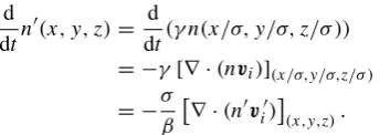
where yˆ00 is eastward, z is a vertical coordinate (positive downward), x andy will be horizontal coordinates, and u is the constant zonal wind shear. By the equations of motion we mean the quasi-neutral ion and current continuity equa-tionsd_dn_t+∇·(nvi)=0 and∇·(n(vi−ve))=0, whereviandve are determined from the steady state momentum equations using the wind field (Eq. 1) and a polarization electric field E. If the spatial scale of the density distribution is increased by a factorσ, then according to Eq. (1) the wind velocity at corresponding points is also increased by the factorσ, and the equations of motion will be satisfied by increasing the polarization electric fields by the same factorσ.

Specifically, consider the rescaled plasma density

n0(x, y, z)=γ n(x/σ, y/σ, z/σ ), (2) and the rescaled ion and electron velocities

v_i,e0 (x, y, z)=βvi,e(x/σ, y/σ, z/σ ), (3) where σ, γ, and β are constants. Plugging into the current continuity equation ∇·(n(vi−ve))=0 we find ∇·(n0(v0_i−v0_e))=0, that is, the rescaled triple(n0,v_i0,v0_e)also satisfies the current continuity equation. To check the ion continuity equation for the pair(n0,v0_i)we compute the time

derivative ofn0, using the assumption that(n,vi)satisfies the ion continuity equation:

d dtn

0_{(x, y, z)=} d

dt(γ n(x/σ, y/σ, z/σ )) = −γ[∇ ·(nvi)](x/σ,y/σ,z/σ ) = −σ

β

∇ ·(n0v_i0)_(x,y,z). (4) Equation (4) shows that the pair(n0,v0

i)satisfies the ion con-tinuity equation whenβ=σ. Therefore, the equations of mo-tion are satisfied by the rescaled quantities defined in Eqs. (2) and (3) if there is a polarization fieldE0_{such thatv}0

i andv 0 e satisfy the steady state momentum equations withβ=σ, us-ing the wind field (Eq. 1).

According to the steady state momentum equations the ion and electron velocities are locally determined, and propor-tional touand the electric fieldE, that is,

if u(x)→αu(x0_{) and E(x)→αE(x}0_),

then vi,e(x)→αvi,e(x0), for anyα, (5) where the notation → is used to mean “is replaced by.” The wind field (Eq. 1) is self-similar in the sense u(x, y, z)=σu(x/σ, y/σ, z/σ ). Therefore, with the wind field (Eq. 1), and a rescaled electric field

E0(x, y, z)=σE(x/σ, y/σ, z/σ ), (6) the relation (5) gives the rescaled velocitiesv0_i,e in Eq. (3), withβ=σ. This shows that the equations of motion are sat-isfied by the rescaled quantities

n0(x, y, z)=γ n(x/σ, y/σ, z/σ ), and

E0(x, y, z)=σE(x/σ, y/σ, z/σ ), (7) for any constantsσandγ, using the wind field (Eq. 1). (Note that choosing γ=1/σ preserves the FLI density under the transformation (2).)

This result holds exactly, for any n, and means that the density fields n and n0 track each other exactly, with the rescaling factorsσ andγ, no matter how nonlinear the evo-lution becomes. If, for example,σ=2, andnis anEs layer with an initial sinusoidal perturbation of wavelengthλ, then n0 is an Es layer with an initial sinusoidal perturbation of wavelength 2λ. The maximum polarization electric field as-sociated withn0 is double the maximum associated withn. Likewise, the maximum vertical scale associated withn0 is double that associated withn, etc.

Therefore, we have in effect derived the power spectrum for the structure generated by theEs layer instability (in sim-plest form), which might apply under an assumption akin to the concept of fully developed turbulence that arises in the theory of turbulent fluids. In this regard, the scaling opera-tion also affects the amplitude of the initial sinusoidal per-turbation. If the amplitude is not rescaled then the derivation above, specifically Eq. (4), is not valid. The interpretation

that we have derived the power spectrum relies on an as-sumption that the final saturation amplitude is not sensitive to the initial perturbation amplitude, which is what we mean by “an assumption akin to the concept of fully developed tur-bulence.” The simulations below will employ the same initial amplitude for all wavelengths, and hence will test this as-sumption.

When there is an F-region winduF, and/or an unsheared meridional winduNin the E-region, then the additional scal-ing relations

u0_F(x, y, z)=σu_F(x/σ, y/σ, z/σ ) and

u0_N(x, y, z)=σ uN(x/σ, y/σ, z/σ ) (8) must be assumed for the above derivation to go through. This is an alteration of the background conditions. Hence, our re-sults concerning the rescaling with wavelength of the maxi-mum electric field, and of the maximaxi-mum vertical scale, do not hold exactly under these more general conditions. We turn now to numerical simulations to verify that the results are at least qualitatively correct, that is, that theEslayer instability creates larger electric fields and more vertical excursion of plasma at longer wavelengths.

2.2 Simulations

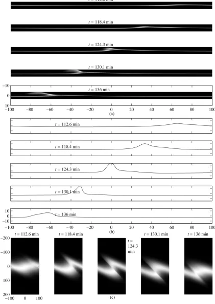
To investigate the wavelength dependence of theEslayer in-stability with F-region and meridional E-region winds, we apply the simulation developed by Cosgrove (2006a). This is a two-dimensional numerical solution of the two-fluid equa-tions, simultaneously covering theEs and F layers, coupled by the assumption that the electric field maps perfectly along the magnetic field B. The conditions are set up to match Fig. 5 of Cosgrove (2006a), with wavelengths of 200 km, 100 km, 50 km, and 25 km. By wavelength we mean the wavelength of the initial seed altitude perturbation, which is given in the F layer. TheEs layer is initially flat. The Es layer is unstable to theEs layer instability, the F layer is unstable to the Perkins instability (Perkins, 1973), and there is a relative horizontal velocity between the two lay-ers of 120 m/s. The latter condition is what is referred to by Cosgrove and Tsunoda (2004) and Cosgrove (2006a) as the non-resonant condition. In this case, and if theEs layer is sufficiently dense, Cosgrove (2006a) found that the role of the Perkins instability is mostly to seed theEs layer insta-bility, and that the interesting electrodynamics comes from the nonlinearity of theEs layer instability. The “sufficiently dense” criteria was found numerically to be6H/6P F&1, where6H is the FLI Hall conductivity of theEs layer, and 6P F is the FLI Pedersen conductivity of the F layer.

3936 R. B. Cosgrove:Es layer instability

4

Cosgrove

E

B

45

45

Northeast

U

p

,

w

it

h

t

ilt

t

o

w

a

rd

s

o

u

th

e

a

s

t

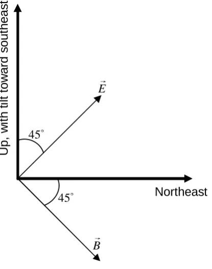
Figure 1: Axis orientation for Figures 2 through 5. The

coordinate axes,

E

~

_{, and}

B

~

_{, all lie in the planes of the figures.}

figure is that the

y

axis is directed upward, and a little

toward the southeast. The

x

axis, however, is exactly

horizontal.

The time periods shown in Figures 2 through 5 are

chosen to bracket the wave-breaking events, which

con-stitute the explosive growth phase of the instability.

The maximum electric field occurs simultaneously with

the wave-breaking event. Before the wave breaking event

there is little visible activity in the layer, and the electric

field is small. After the wave breaking event the electric

field again decreases, and the layer structure becomes

more disorganized. The shorter the wavelength of the

initial seed modulation, the longer it takes for the

wave-breaking event to occur.

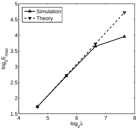
Comparing the electric field plots in Figures 2 through 5

confirms the finding that the maximum electric field

(maximum occurring over the course of the evolution

subsequent to the initial 5 km altitude modulation of

the

F

layer) grows with wavelength. Figure 6 shows

log

-log

plots of the maximum electric field versus the

wavelength of the initial modulation, as found by the

simulations presented in Figures 2 through 5, and by

applying the scaling rule of Section 2.1 (theory). The

horizontal axis of Figure 6 is log

of wavelength in km,

and the vertical axis is log

of maximum electric field

in mV/m. The scaling rule is applied by setting the

theoretical and simulated electric field maxima equal at

λ

= 25 km (log

(25) = 4

.

64), and scaling to the longer

wavelengths. Figure 6 shows that the scaling rule works

well for the first two doublings of the wavelength, but

fails for the third.

The fact that the effect is less than a direct

propor-tionality is consistent with the expectations developed

in Section 2.1, where we noted that a direct

proportion-ality would result only if the

E

layer meridional wind,

and the

F

layer winds, were also rescaled.

An additional factor arises because the simulation

employs a rotational wind shear, and hence does not

have a strictly linear variation of the zonal wind with

altitude. This may be responsible for the large deviation

from linearity observed in Figure 6 between

λ

= 100 km

and

λ

= 200 km, because it is in this wavelength-range

that the maximum altitude excursion of the

E

layer

modulation (which increases with wavelength, along with

the maximum electric field) approaches one-quarter of a

wavelength of the rotational wind shear. The

altitude-excursion approaches the end of the zonal-wind-shear

region, as the approximation sin

ε

≃

_ε

_{begins to break}

down. Also, the meridional wind, which is essential to

the instability (Cosgrove, 2007b), is significantly decreased—

as the altitude excursion moves away from the peak of

the cosine.

With regard to the increase in

F

layer altitude

dis-placement associated with increasing wavelength, we

note that in addition to the fact that the

E

layer

pro-duced electric fields increase with wavelength, the

inter-action time between the two layers also increases with

wavelength. Specifically, since the relative horizontal

velocity (between the

E

and

F

layers) is fixed, a longer

wavelength means that it takes longer for the electric

field seen by a particular piece of

F

layer plasma to be

reversed, due to relative drift. This longer interaction

time, together with the stronger electric fields, creates

an increased

F

layer altitude modulation.

In Figure 7 a possible interaction between large and

small scale excitations of the

E

layer instability is

il-lustrated. The simulation output for the 200 km

wave-length excitation is taken as the initial state for the

E

and

F

layers. Representative of the effects of a

lower-thermospheric gravity wave, we apply a

±

₀

_.

_{25 km}

am-plitude, 25 km wavelength, sinusoidal altitude

modula-tion to the

E

layer density profile at

t

= 203

.

6 minutes,

which is after the breaking wave (seen in Figure 2) has

subsided. The result, shown 12 minutes after the initial

perturbation, is a 25-km-scale modulation of the

polar-ization electric field, which exists over half the

E

layer

extent (over 100 km). This result is reminiscent of

ob-servations (Saito et al., 2007) that show QP-echo-scale

modulation of radar backscatter (assumed to be scatter

from meter scale irregularities produced by a

polariza-tion electric field), within a larger-scale modulapolariza-tion

en-velope that matches the scale of the

F

-region-produced

airglow.

3

Summary of Conclusions and Results

The conclusions and results of this work are

summa-rized as follows:

1. In simplest form, the electric fields and

spatial-scale of an excitation of the

E

layer at any stage

of evolution scale directly with the spatial scale of

Fig. 1. Axis orientation for Figs. 2 through 5. The coordinate axes,

E, andB, all lie in the planes of the figures.

A uniform wind field of 45 m/s to the east, and 22 m/s to the south, is applied in the F-region. There is no background (i.e. not caused by polarization of theEs layer) electric field. A 0.6 km half width Gaussian density profile is located at the zonal wind shear node on the E-region grid, and a 120 km half width Gaussian density profile is located on the F-region grid. The ion-neutral collision frequency is computed from a curve fit to data given by Johnson (1961), with theEs layer located at an altitude of 100 km. The ratio of theEslayer FLI Hall conductivity to the F layer FLI Pedersen conductivity is set to 6H

6P F=1.8. This leads to a ratio ofEs layer FLI

Ped-ersen conductivity to F layer FLI PedPed-ersen conductivity of 6P E

6P F=0.06. Details of the simulation method may be found

in Cosgrove (2006a).

The simulation results are presented in Figs. 2 through 5. The figures show cross sections of theEs layer and F layer densities in grey scale, and the electric field at the equilib-rium altitude of theEs layer. The scales for all figures are in kilometers, except for the y-axis of the electric field figures, which is in mV/m. The orientation of the coordinate axes is summarized in Fig. 1. The axes are defined so that bothB andE lie in the figure plane. The x-axis is northeast, andB makes a 45◦angle with the x-axis, directed from top left to bottom right. The electric fieldEis perpendicular toB, with positive defined from bottom left to top right. The sacrifice for makingBandElie in the plane of the figure is that the y-axis is directed upward, and a little toward the southeast. The x-axis, however, is exactly horizontal.

The time periods shown in Figs. 2 through 5 are chosen to bracket the wave-breaking events, which constitute the explosive growth phase of the instability. The maximum electric field occurs simultaneously with the wave-breaking event. Before the wave breaking event there is little visible activity in the layer, and the electric field is small. After the wave breaking event the electric field again decreases, and the layer structure becomes more disorganized. The shorter the wavelength of the initial seed modulation, the longer it takes for the wave-breaking event to occur.

Comparing the electric field plots in Figs. 2 through 5 con-firms the finding that the maximum electric field (maximum occurring over the course of the evolution subsequent to the initial 5 km altitude modulation of the F layer) grows with wavelength. Figure 6 shows log₂–log₂plots of the maximum electric field versus the wavelength of the initial modulation, as found by the simulations presented in Figs. 2 through 5, and by applying the scaling rule of Sect. 2.1 (theory). The horizontal axis of Fig. 6 is log₂of wavelength in km, and the vertical axis is log₂of maximum electric field in mV/m. The scaling rule is applied by setting the theoretical and simulated electric field maxima equal at λ=25 km (log₂(25)=4.64), and scaling to the longer wavelengths. Figure 6 shows that the scaling rule works well for the first two doublings of the wavelength, but fails for the third.

The fact that the effect is less than a direct proportional-ity is consistent with the expectations developed in Sect. 2.1, where we noted that a direct proportionality would result only if theEs layer meridional wind, and the F layer winds, were also rescaled.

An additional factor arises because the simulation employs a rotational wind shear, and hence does not have a strictly linear variation of the zonal wind with altitude. This may be responsible for the large deviation from linearity observed in Fig. 6 between λ=100 km and λ=200 km, because it is in this wavelength-range that the maximum altitude excur-sion of theEs layer modulation (which increases with wave-length, along with the maximum electric field) approaches one-quarter of a wavelength of the rotational wind shear. The altitude-excursion approaches the end of the zonal-wind-shear region, as the approximation sinε'ε begins to break down. Also, the meridional wind, which is essential to the instability (Cosgrove, 2007b), is significantly decreased – as the altitude excursion moves away from the peak of the co-sine.

With regard to the increase in F layer altitude displacement associated with increasing wavelength, we note that in addi-tion to the fact that theEs layer produced electric fields in-crease with wavelength, the interaction time between the two layers also increases with wavelength. Specifically, since the relative horizontal velocity (between theEs and F layers) is fixed, a longer wavelength means that it takes longer for the electric field seen by a particular piece of F layer plasma to be reversed, due to relative drift. This longer interaction time,

EsLAYER INSTABILITY 5

−100 0 100 −200

−100

0

100

200

(c) (a)

(b) t = 112.6 min t = 118.4 min

t = 124.3 min

t = 130.1 min t = 136 min

−100 −80 −60 −40 −20 0 20 40 60 80 100

−10 0 10

t = 136 min t = 130.1 min t = 124.3 min t = 118.4 min t = 112.6 min

t = 136 min

−100 −80 −60 −40 −20 0 20 40 60 80 100

−10

0

10

t = 130.1 min t = 124.3 min t = 118.4 min t = 112.6 min

Figure 2: Seed wavelength of 200 km with ΣH

ΣP F = 1

._{8. (a)}Eslayer, (b) electric field, and (c)F layer. The axes for all

figures are described in Section 2.2, and summarized in Figure 1.

Fig. 2. Seed wavelength of 200 km with 6H

6P F=1.8. (a)Es layer, (b) electric field, and (c) F layer. The axes for all figures are described in

3938 R. B. Cosgrove:Es layer instability

6 Cosgrove

−100 0 100 −200

−100

0

100

200

t = 177.6 min

−100 −80 −60 −40 −20 0 20 40 60 80 100

−10

0

10

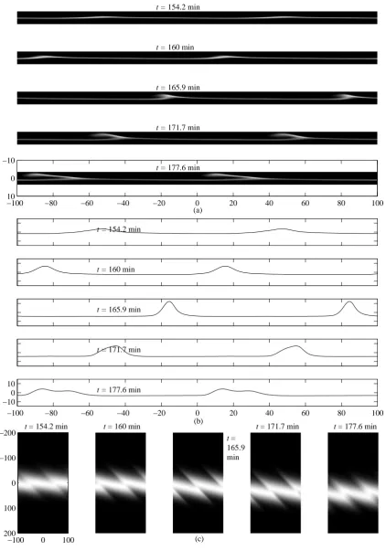
t = 171.7 min t = 165.9 min t = 160 min t = 154.2 min

−100 −80 −60 −40 −20 0 20 40 60 80 100

−10 0 10

t = 177.6 min t = 171.7 min t = 165.9 min t = 160 min t = 154.2 min

(a)

(b)

(c) t = 154.2 min t = 160 min

t = 165.9 min

t = 171.7 min t = 177.6 min

Figure 3: Seed wavelength of 100 km with ΣH

ΣP F = 1.8. (a)Eslayer, (b) electric field, and (c)F layer. The axes for all

figures are described in Section 2.2, and summarized in Figure 1.

Fig. 3. Seed wavelength of 100 km with 6H

6P F=1.8. (a)Es layer, (b) electric field, and (c) F layer. The axes for all figures are described in

Sect. 2.2, and summarized in Fig. 1.

s

−100 0 100 −200

−100

0

100

200

−100 −80 −60 −40 −20 0 20 40 60 80 100

−10 0 10

t = 192.5 min t = 186.7 min t = 180.8 min t = 175 min t = 169.1 min

t = 192.5 min

−100 −80 −60 −40 −20 0 20 40 60 80 100

−10

0

10

t = 186.7 min t = 180.8 min t = 175 min t = 169.1 min

(a)

(b)

(c) t = 169.1 min t = 175 min

t = 180.8 min

t = 186.7 min t = 192.5 min

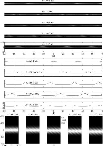
Figure 4: Seed wavelength of 50 km with ΣH

ΣP F = 1

._{8. (a)}Eslayer, (b) electric field, and (c)F layer. The axes for all

figures are described in Section 2.2, and summarized in Figure 1.

Fig. 4. Seed wavelength of 50 km with 6H

6P F=1.8. (a)Es layer, (b) electric field, and (c) F layer. The axes for all figures are described in

3940 ₈ R. B. Cosgrove:E_Cosgroves layer instability

−100 0 100 −200

−100

0

100

200

(c) (b)

−100 −80 −60 −40 −20 0 20 40 60 80 100

−10 0 10

t = 198.6 min t = 192.7 min t = 186.8 min t = 180.9 min t = 175 min

(a) t = 198.6 min

−100 −80 −60 −40 −20 0 20 40 60 80 100

−10

0

10

t = 192.7 min t = 186.8 min t = 180.9 min t = 175 min

t = 175 min t = 180.9 min

t = 186.8 min

t = 192.7 min t = 198.6 min

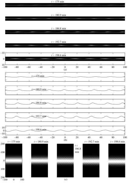
Figure 5: Seed wavelength of 25 km with ΣH

ΣP F = 1.8. (a)Eslayer, (b) electric field, and (c)F layer. The axes for all

figures are described in Section 2.2, and summarized in Figure 1.

Fig. 5. Seed wavelength of 25 km with 6H

6P F=1.8. (a)Es layer, (b) electric field, and (c) F layer. The axes for all figures are described in

Sect. 2.2, and summarized in Fig. 1.

together with the stronger electric fields, creates an increased F layer altitude modulation.

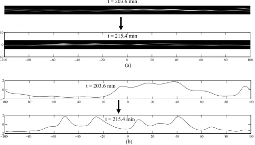
In Fig. 7 a possible interaction between large and small scale excitations of theEslayer instability is illustrated. The simulation output for the 200 km wavelength excitation is taken as the initial state for theEs and F layers. Represen-tative of the effects of a lower-thermospheric gravity wave, we apply a ±0.25 km amplitude, 25 km wavelength, sinu-soidal altitude modulation to the Es layer density profile att=203.6 min, which is after the breaking wave (seen in Fig. 2) has subsided. The result, shown 12 min after the ini-tial perturbation, is a 25-km-scale modulation of the polar-ization electric field, which exists over half theEs layer ex-tent (over 100 km). This result is reminiscent of observations (Saito et al., 2007) that show QP-echo-scale modulation of radar backscatter (assumed to be scatter from meter scale ir-regularities produced by a polarization electric field), within a larger-scale modulation envelope that matches the scale of the F-region-produced airglow.

3 Summary of conclusions and results

The conclusions and results of this work are summarized as follows:

1. In simplest form, the electric fields and spatial-scale of an excitation of theEs layer at any stage of evolution scale directly with the spatial scale of the initial excita-tion. Specifically, when the initial excitation is rescaled as

n(t0, x, y, z)→

1

σn(t0, x/σ, y/σ, z/σ ) (9) (which rescales the wavelength asλ→σ λ), then E(t, x, y, z)→σE(t, x/σ, y/σ, z/σ ) and

n(t, x, y, z)→ 1

σn(t, x/σ, y/σ, z/σ )

for any later timet.

2. Under more realistic assumptions, simulations confirm that the electric fields and spatial-scale of the modes of theEs layer instability increase with wavelength. The increase is significant, but not as rapid as by direct pro-portionality.

3. The increased electric fields, together with an increased interaction time, lead to a significant increase with wavelength of the F layer structuring associated with theEs layer instability.

Items 1 through 3 suggest that the short wavelength (∼20 km) modes of theEs layer instability, which have the largest linear growth rate, may have little effect on the F

4 5 6 7 8

1.5 2 2.5 3 3.5 4 4.5 5 log 2λ log 2 E max Simulation Theory

Figure 6: log₂-log₂ plots of the peak electric field versus

wavelength, as determined by the scaling rule of Section 2.1 (theory), and by the simulations presented in Figures 2

through 5. The horizontal axis is log₂of wavelength in km,

and the vertical axis is log₂of electric field in mV/m. The

scaling rule is applied by setting the theoretical and

simu-lated electric field equal at λ_{= 25 km, and scaling to the}

longer wavelengths.

the initial excitation. Specifically, when the initial excitation is rescaled as

n(t0, x, y, z)→ 1

σn(t0, x/σ, y/σ, z/σ)

(which rescales the wavelength asλ→_{σλ), then}

~

E(t, x, y, z)→_{σ ~E(t, x/σ, y/σ, z/σ) and}

n(t, x, y, z)→ 1

σn(t, x/σ, y/σ, z/σ)

for any later timet.

2. Under more realistic assumptions, simulations con-firm that the electric fields and spatial-scale of the modes of the Es layer instability increase with

wavelength. The increase is significant, but not as rapid as by direct proportionality.

3. The increased electric fields, together with an creased interaction time, lead to a significant in-crease with wavelength of theF layer structuring associated with theEs layer instability.

Items 1 through 3 suggest that the short wavelength (∼_{20 km) modes of theEs layer instability, which have}

the largest linear growth rate, may have little effect on theF layer. In fact, the effect shown in Figure 5 is an exaggeration, since the largest growth rate modes were

found by Cosgrove (2006b) to occur when the electric field produced by the Es layer is partially decoupled

from theF layer, due to short wavelength reduction in the efficiency of mapping along B~. This effect is not accounted for in the simulations.

On the other hand, the longer the wavelength, the larger the polarization field that impacts the F layer, and the longer time it has to act. Therefore, we might expect that the longest wavelength that can be effec-tively initiated in the Es layer, due to the operative

seeding mechanism, and due to the finite size of theEs

layer, will be what is observed in theF layer.

An illustration of a possible interaction between large and small scale excitations is shown in Figure 7, where it is seen that the large-scale excitation appears as an envelope for the smaller-scale excitation. This result is reminiscent of observations by Saito et al. (2007).

In summary, these results seem to be consistent with the observations of Es and F layer frontal structures.

The short wavelength modes are seen in the Es layer,

both because they have the largest growth rate, and be-cause the long wavelength modes are difficult to observe. The latter is due both to the limited horizontal scale of

Eslayer observation techniques, and to the fact that for

long wavelength modes the evolution becomes strongly nonlinear before the altitude modulation becomes an appreciable fraction of the wavelength. The long wave-length modes are observed in theF layer because they are associated with larger polarization fields, and be-cause the fields have a longer interaction time with the

F layer plasma. TheF layer evolution is less nonlinear, and produces altitude modulations that are an appre-ciable fraction of the wavelength, which can be observed by optical techniques with a large horizontal coverage.

In interpreting the simulation results, it is impor-tant to recognize that we have analyzed the electrody-namics of the coupled Es and F layer system under

the assumption that the external inputs are small, and act as mere “seeds”. It is possible, in fact likely, that the external inputs are large. In such case the external inputs may dominate the dynamics. Hence, in the lan-guage of network theory, our result should be regarded as an analysis of the coupled Es and F layer system

response function. To obtain the response in an actual case scenario the drivers must be applied to the system response function. We make no attempt to do this in the present work. It is interesting that some characteristics of the observed phenomena match the characteristics of the system response function, but a complete analysis should consider application of the drivers.

Therefore, none of the assertions given above should be interpreted as a denial of the assertion made by Larsen et al. (2007) that neutral dynamics is the domi-nant driver behind the generation ofEs layer

polariza-tion electric fields, and QP echoes. We have merely sup-plied an analysis of the electrodynamical system func-tion, as a step toward analysis of the driven system, that is, driven by waves or disturbances in the neutral

Fig. 6. log₂-log₂plots of the peak electric field versus wavelength, as determined by the scaling rule of Sect. 2.1 (theory), and by the simulations presented in Figs. 2 through 5. The horizontal axis is log₂of wavelength in km, and the vertical axis is log₂of electric field in mV/m. The scaling rule is applied by setting the theoretical and simulated electric field equal atλ=25 km, and scaling to the longer wavelengths.

layer. In fact, the effect shown in Fig. 5 is an exaggeration, since the largest growth rate modes were found by Cosgrove (2006b) to occur when the electric field produced by theEs layer is partially decoupled from the F layer, due to short wavelength reduction in the efficiency of mapping alongB. This effect is not accounted for in the simulations.

On the other hand, the longer the wavelength, the larger the polarization field that impacts the F layer, and the longer time it has to act. Therefore, we might expect that the longest wavelength that can be effectively initiated in theEs layer, due to the operative seeding mechanism, and due to the finite size of theEslayer, will be what is observed in the F layer.

An illustration of a possible interaction between large and small scale excitations is shown in Fig. 7, where it is seen that the large-scale excitation appears as an envelope for the smaller-scale excitation. This result is reminiscent of obser-vations by Saito et al. (2007).

3942 R. B. Cosgrove:Es layer instability

10

Cosgrove

−100 −80 −60 −40 −20 0 20 40 60 80 100

−10

0

10

t = 203.6 min

t = 215.4 min

−100 −80 −60 −40 −20 0 20 40 60 80 100

−2 0 2

−100 −80 −60 −40 −20 0 20 40 60 80 100

−2 0 2

t = 215.4 min

t = 203.6 min

(a)

(b)

Figure 7: The effects of a secondary, 25 km wavelength seeding of theEslayer (e.g. by a gravity wave), after the 200 km

seeding (by theF _{layer) has run its’ course. The times shown are measured from the initial 200 km seeding, except note}

that a±₀.25 km amplitude, 25 km wavelength modulation has been imposed on the figures labeled t = 203.6 minutes. Plasma density images are shown in panel (a), and the corresponding electric fields are shown in panel (b). The axes for all figures are described in Section 2.2, and summarized in Figure 1.

atmosphere.

When Σ

/

Σ

.

1 the

E

layer is stable. The

simulations of the system response function apply only

in the case when the

E

layer is unstable. However,

the theoretical development of Section 2.1 makes no

as-sumption regarding stability. Hence, it is probable that

even when the layer is stable longer wavelength drivers

produce larger amplitude responses. In addition, it is

clear that even when the

E

layer is stable it is easiest to

excite waves aligned in the direction that is preferential

for the instability.

Acknowledgements:

This material is based upon

work supported by the National Science Foundation

un-der Grant No. 0436568. The author thanks Roland

Tsunoda for valuable discussions.

References

Behnke, R.,

F

layer height bands in the nocturnal

ionosphere over Arecibo, J. Geophys. Res., 84,

974, 1979.

Cathey, E.H., Some midlatitude sporadic-

E

results

from the Explorer 20 satellite, J. Geophys. Res.,

74, 2240, 1969.

Cosgrove, R.B., and R.T. Tsunoda, A

direction-dependent instability of sporadic-

E

layers in

the nighttime midlatitude ionosphere, Geophys.

Res. Lett., 29(18), 1864, 2002.

Cosgrove, R.B., and R.T. Tsunoda, Simulation of

the nonlinear evolution of the sporadic-

E

layer

instability in the nighttime midlatitude

iono-sphere, J. Geophys. Res., 108(A7), 1283, 2003.

Cosgrove, R.B., and R.T. Tsunoda, Instability of

the

E

-

F

coupled nighttime midlatitude

iono-sphere, J. Geophys.

Res., 109, A04305,

doi:10.1029/2003JA010243, 2004.

Cosgrove, R.B., Generation of mesoscale

F

layer

structure and electric fields by the combined

Perkins and

E

layer instabilities, in

simula-tions, Ann.

Geophys., 25, pp.

1579-1601,

www.ann-geophys.net/25/1579/2007/, 2007a.

Cosgrove, R.B., Wavelength dependence of the

lin-ear growth rate of the

E

layer instability,

Ann. Geophys., 25, pp. 1311-1322,

www.ann-geophys.net/25/1311/2007/, 2007b.

Fukao, S., M.C. Kelley, T. Shirakawa, T. Takami,

M. Tamamoto, T. Tsuda, and S. Kato,

Turbu-lent upwelling of the midlatitude ionosphere, 1,

Observational results by the MU radar, J.

Geo-phys. Res. 96, 3725, 1991.

Fig. 7. The effects of a secondary, 25 km wavelength seeding of theEslayer (e.g. by a gravity wave), after the 200 km seeding (by the F layer) has run its course. The times shown are measured from the initial 200 km seeding, except note that a±0.25 km amplitude, 25 km wavelength modulation has been imposed on the figures labeledt=203.6 min. Plasma density images are shown in panel (a), and the corresponding electric fields are shown in panel (b). The axes for all figures are described in Sect. 2.2, and summarized in Fig. 1.

wavelength modes are observed in the F layer because they are associated with larger polarization fields, and because the fields have a longer interaction time with the F layer plasma. The F layer evolution is less nonlinear, and produces altitude modulations that are an appreciable fraction of the wave-length, which can be observed by optical techniques with a large horizontal coverage.

In interpreting the simulation results, it is important to rec-ognize that we have analyzed the electrodynamics of the cou-pledEsand F layer system under the assumption that the ex-ternal inputs are small, and act as mere “seeds”. It is possible, in fact likely, that the external inputs are large. In such case the external inputs may dominate the dynamics. Hence, in the language of network theory, our result should be regarded as an analysis of the coupledEs and F layer system response function. To obtain the response in an actual case scenario the drivers must be applied to the system response function. We make no attempt to do this in the present work. It is in-teresting that some characteristics of the observed phenom-ena match the characteristics of the system response func-tion, but a complete analysis should consider application of the drivers.

Therefore, none of the assertions given above should be interpreted as a denial of the assertion made by Larsen et al. (2007) that neutral dynamics is the dominant driver be-hind the generation ofEs layer polarization electric fields, and QP echoes. We have merely supplied an analysis of the electrodynamical system function, as a step toward analysis of the driven system, that is, driven by waves or disturbances in the neutral atmosphere.

When6H/6P F.1 theEslayer is stable. The simulations of the system response function apply only in the case when theEs layer is unstable. However, the theoretical develop-ment of Sect. 2.1 makes no assumption regarding stability. Hence, it is probable that even when the layer is stable longer wavelength drivers produce larger amplitude responses. In addition, it is clear that even when theEs layer is stable it is easiest to excite waves aligned in the direction that is prefer-ential for the instability.

Acknowledgements. This material is based upon work supported by the National Science Foundation under Grant No. 0436568. The au-thor thanks Roland Tsunoda for valuable discussions.

Topical Editor M. Pinnock thanks S. Saito and another anony-mous referee for their help in evaluating this paper.

References

Behnke, R.:Flayer height bands in the nocturnal ionosphere over Arecibo, J. Geophys. Res., 84, 974–978, 1979.

Cathey, E. H.: Some midlatitude sporadic-Eresults from the Ex-plorer 20 satellite, J. Geophys. Res., 74, 2240–2247, 1969. Cosgrove, R. B. and Tsunoda, R. T.: A direction-dependent

instabil-ity of sporadic-Elayers in the nighttime midlatitude ionosphere, Geophys. Res. Lett., 29(18), 1864–1867, 2002.

Cosgrove, R. B. and Tsunoda, R. T.: Simulation of the nonlin-ear evolution of the sporadic-E layer instability in the night-time midlatitude ionosphere, J. Geophys. Res., 108(A7), 1283, doi:10.1029/2002JA009728, 2003.

Cosgrove, R. B. and Tsunoda, R. T., Instability of theE-F cou-pled nighttime midlatitude ionosphere, J. Geophys. Res., 109, A04305, doi:10.1029/2003JA010243, 2004.

Cosgrove, R. B.: Generation of mesoscale F layer structure and electric fields by the combined Perkins andEslayer instabilities, in simulations, Ann. Geophys., 25, 1579–1601, 2007a,

http://www.ann-geophys.net/25/1579/2007/.

Cosgrove, R. B.: Wavelength dependence of the linear growth rate of theEs layer instability, Ann. Geophys., 25, 1311–1322, 2007b,

http://www.ann-geophys.net/25/1311/2007/.

Fukao, S., Kelley, M. C., Shirakawa, T., Takami, T., Tamamoto, M., Tsuda, T., and Kato, S.: Turbulent upwelling of the midlatitude ionosphere, 1, Observational results by the MU radar, J. Geo-phys. Res., 96, 3725–3746, 1991.

Fukao, S., Yamamoto, M., Tsunoda, R. T., Hayakawa, H., and Mukai, T.: The SEEK (Sporadic-E Experiment over Kyushu) Campaign, Geophys. Res. Lett., 25, 1761–1764, 1998.

Garcia, F. J., Kelley, M. C., and Makela, J. J.: Airglow observations of mesoscale low-velocity traveling ionospheric disturbances at midlatitudes, J. Geophys. Res., 105, 18 407–18 415, 2000. Goodwin, G. L.: The dimensions of some horizontally movingEs

-region irregularities, Planet. Space. Sci., 14, p. 759, 1966. Goodwin, G. L. and Summers, R. N.: Es layer characteristics

de-termined from spaced ionosondes, Planet Space Sci., 18, 1417– 1432, 1970.

Johnson, F. S. (Ed.): The Satelite Environment Handbook, Stanford University Press, Stanford, CA, 1961.

Hysell, D. L., Larsen, M. F., and Zhou, Q. H.: Common volume co-herent and incoco-herent scatter radar observations of mid-latitude sporadic E-layers and QP echoes, Ann. Geophys., 22, 3277– 3290, 2004,

http://www.ann-geophys.net/22/3277/2004/.

Kubota, M., Fukunishi, H., and Okana, S.: Characteristics of medium- and large-scale TIDs over Japan derived from OI 630-nm nightglow observation, Earth Planet. Space, 53, 741–751, 2001.

Larsen, M. F., Hysell, D. L., Zhou, Q. H., Smith, S. M., Friedman, J., and Bishop, R. L.: Imaging coherent scatter radar, incoher-ent scatter radar, and optical observations of quasiperiodic struc-tures associated with sporadicElayers, J. Geophys. Res., 112, A06321, doi:10.1029/2006JA012051, 2007.

Otsuka, Y., Onoma, F., Shiokawa, K., Ogawa, T., Yamamoto, M., and Fukao, S.: Simultaneous observations of nighttime medium-scale traveling ionospheric disturbances andEregion field-aligned irregularities at midlatitude, J. Geophys. Res., 112, A06317, doi:10.1029/2005JA011548, 2007.

Perkins, F.: SpreadFand ionospheric currents, J. Geophys. Res., 78, 218–226, 1973.

Pfaff, R., Yamamoto, M., Marionni, P., Mori, H., and Fukao, S.: Electric field measurements above and within a sporadic-Elayer, Geophys. Res. Lett., 25, 1769–1772, 1998.

Pfaff, R., Freudenreich, H., Yokoyama, T., Yamamoto, M., Fukao, S., Mori, H., Ohtsuka, S., and Iwagami, N.: Electric field mea-surements of DC and long wavelength structures associated with sporadic-E layers and QP radar echoes, Ann. Geophys., 23, 2319–2334, 2005,

http://www.ann-geophys.net/23/2319/2005/.

Saito, A., Fukao, S., and Miyazaki, S.: High resolution mapping of TEC perturbations with the GSI GPS network over Japan, Geo-phys. Res. Lett., 25, 3079–3082, 1998.

Saito, A., Nishimura, M., Yamamoto, M., Fukao, S., Kubota, M., Shiokawa, K., Otsuka, Y., Tsugawa, T., Ogawa, T., Ishii, M., Sakanoi, T., and Miyazaki, S.: Traveling ionospheric distur-bances detected in the FRONT campaign, Geophys. Res. Lett., 28(4), 689–692, 2001.

Saito, S., Yamamoto, M., Hashiguchi, H., Maegawa, A., and Saito, A.: Observational evidence of coupling between quasi-periodic echoes and medium scale traveling ionospheric disturbances, Ann. Geophys., 25, 2185–2194, 2007,

http://www.ann-geophys.net/25/2185/2007/.

Shiokawa, K., Ihara, C., Otsuka, Y., and Ogawa, T.: Statistical study of nighttime medium-scale travelling ionospheric disturbance using midlatitude airglow images, J. Geophys. Res., 108(A1), 1052–1058, doi:1029/2002JA009491, 2003.

Tsugawa, T., Otsuka, Y., Coster, A. J., and Saito, A.: Medium-scale travelling ionospheric disturbances detected with dense and wide TEC maps over North America, Geophys. Res. Lett., 34, L22101, doi:10.1029/2007GL031663, 2007.

Tsunoda, R., Fukao, S., and Yamamoto, M.: On the origin of quasi-periodic radar backscatter from midlatitude sporadicE, Radio Sci., 29, 349–365, 1994.

Tsunoda, R. T. and Cosgrove, R. B.: Coupled electrodynamics in the nighttime midlatitude ionsphere, Geophys. Res. Lett., 28, 4171–4174, 2001.

Tsunoda, R. T., Cosgrove, R. B., and Ogawa, T.: Azimuth-dependentEs layer instability: A missing link found, J. Geo-phys. Res., 109, A12303, doi:10.1029/2004JA010597, 2004. Yamamoto, M., Fukao, S., Woodman, R. F., Ogawa, T., Tsuda, T.,

and Kato, S.: Midlatitude E-region field-aligned irregularities observed with the MU radar, J. Geophys. Res., 96(A9), 15 943– 15 949, 1991.

Yamamoto, M., Komoda, N., Fukao, S., Tsunoda, R., Ogawa, T., and Tsuda, T.: Spatial structure of theEregion field-aligned ir-regularities revealed by the MU radar, Radio Sci., 29(1), 337– 347, 1994.

Yamamoto, M., Kumura, F., Fukao, S., Tsunoda, R. T., Igarashi, K., and Ogawa, T.: Preliminary results from joint measurements of E-region field-aligned irregularities using the MU radar and the frequency-agile radar, J. Atmos. Solar Terr. Phys., 59, 1655– 1663, 1997.