Copyright © 2019 (Chris Wells, Dhavan V. Shah, Jon C. Pevehouse, Jordan Foley, Josephine Lukito, Ayellet Pelled, and JungHwan Yang). Licensed under the Creative Commons Attribution Non-commercial No Derivatives (by-nc-nd). Available at http://ijoc.org.
The Temporal Turn in Communication Research:
Time Series Analyses Using Computational Approaches
CHRIS WELLS
1Boston University, USA
DHAVAN V. SHAH
JON C. PEVEHOUSE
JORDAN FOLEY
JOSEPHINE LUKITO
AYELLET PELLED
University of Wisconsin–Madison, USA
JUNGHWAN YANG
University of Illinois at Urbana-Champaign, USA
Some of the most pioneering work in our field is occurring where emerging computational approaches are meeting time series analytic techniques. Combining these methods is helping scholars improve our understanding of phenomena as varied as news and issue attention cycles, physiological responses to communication exposure, changes in mass opinion, and the dynamics between social media and legacy news media. In this article, we summarize the current state of computational communication science techniques to generate sequential data for use in time series analysis and suggest directions for further development. In particular, we consider the long-standing place of temporal dynamics for our field’s main theories; overview recent work combining computational science with time series analysis; present narrative accounts of two major research programs in this area; and review techniques of time series analysis, including major concerns for communication researchers working in the area.
Chris Wells: [email protected] Dhavan V. Shah: [email protected]
Jon C. Pevehouse: [email protected] Jordan Foley: [email protected]
Josephine Lukito: [email protected] Ayellet Pelled: [email protected] JungHwan Yang: [email protected] Date submitted: 2018–10–03
1 This work was supported by the Vice Chancellor for Research and Graduate Education at the UW–Madison
Keywords: time series, computational, agenda-setting, flow, methods, ARIMA, media effects, Granger, dynamics
Communication research has long built time into its conceptions of influence. Yet, relative to allied fields, ours has not been especially advanced about explicating time’s functions theoretically or empirically (Yanovitzky & VanLear, 2008). To be sure, solid research examining temporal dynamics has been present for decades: See the cross-lagged correlations of early agenda-setting research and its refinements (McCombs & Shaw, 1972), multidose priming studies (Iyengar & Kinder, 1987), modeling opinion dynamics using overtime shifts in news content (Fan & Tims, 1989), and rolling cross-sectional analyses of opinion (Johnston, Blais, Brady, & Crete, 1992). But more often, time has been set aside for the limitation section of cross-sectional studies.
Today, we stand on the cusp of a new phase in our field’s opportunities to incorporate temporal dynamics into research, which is a product of two advances. One is the development of computational social science (Lazer et al., 2009), and more specifically computational communication science techniques for generating sequential data (Shah et al., 2016). The emergence of these computational research techniques alongside novel sources of data and methods has opened new frontiers for examining a variety of communication dynamics in fine-grained temporal detail. Second, in recent years, communications scholars’ awareness of and borrowings from other fields with expertise in modeling temporal dynamics have grown greatly. At the intersection of these developments is a burgeoning domain we call computational communication science using time series analysis.
The aim of this article is to (a) synthesize the work linking computationally generated data streams with other temporal data, (b) specify appropriate techniques for the analysis of this data, (c) draw attention to challenges in these processes, and (d) provide resources for scholars wishing to learn more about these intersecting approaches. The article is divided into four sections. In the first, we present theoretical considerations explaining why time is conceptually important to communication research, both historically and today; the second is an overview of pioneering research in computational communication science employing time series modeling; the third offers a narrative account of two research programs in this area; and the fourth includes greater detail about relevant time series analysis techniques. We conclude by returning to the promise of merging computational approaches with time series analytic techniques.
I. Time in Communication Research
Time, Process, and Causation
includes communication exposure. Indeed, the words that animate our field—effect, flow, influence, dynamic, cycle—reveal our understanding of communication as a process, and processes have temporal dimensions (Box-Steffensmeier, Freeman, Hitt, & Pevehouse, 2014). The perspective of time series analysis can help expand our notions of time’s role in these dynamics. We see several ways in which we can become more attentive to time in our field.
Though we often obscure it, many of communication’s major models are causal in nature. Students learn to think through establishing causality by identifying correlations, accounting for covariates, and determining temporal order. Until recently, the last of these has often been the most difficult to establish. With the spread of computationally derived data sets and advanced time series modeling techniques, this is sure to change, intensifying our need to remain aware of the other assumptions built into research of this kind. As we take advantage of these tools, we must be careful not to reduce our theoretical vistas to reductive causal stories. Responding to this tendency, Lang and Ewoldsen (2010) write,
If, as a discipline, we continue the habit of thinking that scientific, quantitative research in communication must be focused on effects, we will never begin the complex and necessary work of theorizing about long-term, systemic, complex, dynamic, interactive processes that make up the science of how communication works. (p. )
A more expansive conception of time is essential to understanding the dynamic processes that connect the communication system.
Further, most models are conceived in terms of the simplest causal temporality—linearity—which is often a usefully parsimonious, if narrow, starting point (Hindman, 2015). More sophisticated time series techniques can help us test and inform other theoretical ideas about how dynamics play out. Some may not be linear, but instead rely on an accumulated effect over time (as cultivation theory postulates); many effects have some kind of decay function by which they disappear, a tendency often absent from communication theories (cf. Fan, 1988). Still other effects may not manifest immediately, only appearing after time passes, and yet others may require surpassing a threshold to manifest (Gotlieb, Scholl, Ridout, Goldstein, & Shah, 2017).
Another temporal simplification is an assumption of temporal stability: that effects play out at a steady rate at different moments in time. Regression-based time series analysis makes this assumption in the sense that it averages across all time points as though they were the same. In reality, not all time is created equal: As Dayan and Katz (1992) demonstrated decades ago, media events are extraordinary moments that attract disproportionate attention and effects, even in the digital age (e.g., Shah et al., 2016).
general elections campaign. Here, communication may take inspiration from punctuated equilibrium theory’s (True, Jones, & Baumgartner, 1999) call to distinguish moments of stability from those of rapid change; the notion of media storms having unique properties and unique effects is a helpful step in this direction (Boydstun, Hardy, & Walgrave, 2014).
Complexity and Instability, Unpredictability and Instantaneity
We must also remain aware of the many ways in which time’s place in communication, and in society, is becoming more complicated. Sociologists of the last two decades have described the changing nature of time resulting from the conditions of postindustrial, digitally networked society. Whether “liquid modernity,” “timeless time,” or “time-space distanciation,” these notions assert that individuals and social practices are being forced to adapt to communication processes approaching instantaneity. Moreover, people at different locations within the network society vary in their ability to adapt to, and benefit from, these new conditions (Castells, 2010). These are dynamics that directly impact the lived experiences of creators and audiences of communication and shape the practice of communication itself.
Chadwick’s (2017) is one of the richest articulations of the implications of time’s new nature for political communication. His “political information cycle” makes clear that politics can now play out in near simultaneous real time, incorporating myriad actors who emerge from unexpected corners of the hybrid media system. When combined with time-stamped digital media artifacts, time series analyses offer techniques for studying behaviors that occur in micro-increments of seconds or milliseconds, though the simultaneity and complexity of the contemporary media system may defy untangling.
This spontaneity and unpredictability challenges theories of regularity and routinization. Today, news comes out all the time at a relentless pace and is immediately met with responses by a wide range of communicative actors. Yet, our theoretical frameworks—as well as our often regression-based empirical techniques—are only beginning to come to terms with this complexity (Karlsson & Strömbäck, 2010).
We present these considerations as a call for communication scholars to attend to matters of time more conscientiously in both theory and method and to encourage empirical modesty as we exploit new tools for measuring and modeling communication dynamics.
II. Time Series and Computational Methods in Communication Research
and inferences from these data (Shah, Cappella, & Neuman, 2015). More detail on the unique properties of temporally ordered data is offered in Section IV and supplementary materials.2
Further, data created through “always on” (Salganik, 2017) computational processes frequently include records of the time of creation. Unlike data collection from the prior era, where the main source of data was one-time responses to a survey, interview, or experiment, digital trace data inherently lend themselves to time series analysis. Increasingly, that synthesizes multiple forms of data—for example, event data, news coverage, public opinion, and/or social media texts—into a unified data set amenable to new forms of modeling.
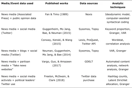
[image:5.612.91.521.323.610.2]In this section, we present an overview of ways in which computationally collected or derived data are being used within time series techniques (see Table 1 and discussion below). Though space constrains us from comprehensively treating the computational approaches mentioned here, more detail on them can be found in the article’s supplementary materials.
Table 1. Illustrative Uses of Computationally Derived Data Sets in Time Series Analysis.
Media/Event data used Published works Data sources Analytic
techniques
News media (Associated Press) + public opinion data
Fan & Tims (1989) Nexis Ideodynamic model, computer-assisted syntactical coding
News media + social media (Twitter)
Guggenheim, Mo Jang, Bae, & Neuman (2015)
Sysomos, Topsy Keyword proportion, Granger, VAR
Conway, Kenski, & Wang (2015)
Lexis, ProQuest, Twitter API
Wordstat, correlation analysis
News media + blogs + social media (Twitter)
Neuman, Guggenheim, Mo Jang, & Bae (2014)
Sysomos, Topsy VAR, Granger
News media + partisan media + “fake news websites”
Vargo, Guo, & Amazeen (2017)
GDELT Automated content analysis, network analysis, Granger
News media + social media activists + political leaders’ Twitter use
Freelon, McIlwain, & Clark (2018) Twitter data purchase Hashtag counts, Latent Dirichlet allocation, Granger
News event (presidential debate) + social media (Twitter)
Shah et al. (2016) C-SPAN, Twitter API Keyword counts, Granger, VAR
Newspapers + search trends Boydstun, Hardy, & Walgrave (2014)
Human collection of newspapers, Google
Trends
Human content analysis, univariate time series analysis
Physiological + TV Soroka & McAdams (2015)
Skin conductance, heart rate, TV news
segments
ANCOVA, OLS regression
Online news (msm + niche) + search trends
Gruszczynski & Wagner (2017)
MemeTracker, Google Trends
VAR, Granger
TV + public opinion Searles & Smith (2016) News Coverage Index, NAES
VAR, Granger
Newspapers + news events (death penalty) + public opinion
Baumgartner, De Boef, & Boydstun (2008)
Lexis, Gallup/Roper VAR, Granger, error-correction models
Democratization and communication technology diffusion
Mays & Groshek (2017) Polity data series; World Bank, International Telecommunication
Union data
ARIMA, selected case study analysis
Text as Data
Within the field of communication, much of the innovation in computational time series research is occurring in the area of text processing; this is largely because computational tools enable the processing of the large volumes of text necessary for multi-timepoint analyses (Schwartz & Ungar, 2015). This possibility was emergent even 30 years ago, as Fan’s work on tracking change in media content using time series methodology and text-coding methods demonstrated (Fan, 1988; Shah, Watts, Domke, & Fan, 2002).
Variations on simple counts have served as the basis for more significant headway in the area of intermedia agenda setting. Neuman, Guggenheim, Mo Jang, and Bae (2014) derived topical keyword lists using open-ended responses to American National Election Studies surveys, then counted mentions of those issues from traditional media coverage, Twitter posts, blogs, and discussion board conversations to test how the dynamics of public attention differ across topics. Guo and Vargo (2018) measured the co-occurrence of candidate and topic-word mentions to derive the “issue ownership networks” of the 2016 U.S. presidential campaign. Modeling the shifts in those networks in different media over time offered insight into the agenda-setting capacities of various media (see also Harder, Sevenans, & Van Aelst, 2017). Combining human content analysis of text with factor analyses conducted over time, Baumgartner, De Boef, and Boydstun (2008) automated the identification of issue frames and how they change over time.
Machine learning and advanced natural language processing techniques have further increased the range of variables that can be derived from text data. These include classification tasks used to evaluate whether a text or speaker fits into a given category, such as “positive” or “negative,” “liberal” or “conservative” (see Petchler & Gonzalez-Bailon, 2015, for an overview). This makes it possible to analyze more complete concepts that do not rely on repeat uses of words or phrases (Grimmer & Stuart, 2013). Once data are classified and labeled (e.g., for sentiment), they can be analyzed to see how discourse changes temporally (e.g., sentiment about a politician over the course of his or her term). Importantly, these data can then be combined with nontext data to understand the antecedents and consequences of language-in-communication. For example, researchers found a significant temporal correlation between tweet sentiment and Obama’s support rate during the 2008 presidential election and his job approval in surveys in 2009 (O’Connor, Balasubramanyan, Routledge, & Smith, 2010).
Other studies have used unsupervised machine learning techniques to identify key issues in discourse and to analyze the presence (or absence) of topics over time. For example, Cerchiello and Nicola (2018) analyzed a corpus of economic news stories using structural topic modeling, an unsupervised machine learning strategy, and then used Granger causality tests to analyze the spread of financial news stories across different countries. In another analysis of economic news (but focusing on stock markets), Strycharz, Strauss, and Trilling (2018) found that certain topics positively Granger-caused stock price fluctuations.
Multiple computational text analysis tools can be used to extract different types of information from text. Freelon et al. (2018), for example, used both a keyword strategy and topic modeling. Strycharz et al. (2018) used both Latent Dirichlet Allocation (LDA) topic modeling and sentiment classification to understand news about stock markets. These studies show that time series methods can be used to analyze different layers of text data, enhancing the analytical use of computationally analyzed text.
Physiological Measures
Networks and Connections
In network analysis, although researchers have acknowledged that the composition and structure of networks may change over time, they have typically ignored the temporal dynamics when the network process is in a steady state (Borge-Holthoefer & Gonzalez-Bailon, 2017; Snijders, 2005). However, a myriad of digital trace data coming from online forums, e-mail, and social media provide not only information about the relationships of the interaction, but also moment-by-moment time stamps (Lazer et al., 2009). In addition, the speed of online communications, such as the emergence of memes (Weng, Menczer, & Ahn, 2013), mass protest organized with mobile interactions (Chan & Fu, 2017), and a real-time response from social media to a televised national event (Shah et al., 2016), can accelerate the rate of change in network topology. Computational social scientists suggest inspecting time-evolving networks by incorporating more sophisticated methods, such as temporal exponential random graph models, stochastic actor-based models, or continuous-time Markov chains, or simply providing multislice representations of networks (Borge-Holthoefer & Gonzalez-Bailon, 2017).
Despite the diversity of time series applications by political communication scholars, the methodological literature remains sparse. We believe that more concerted attention to time series methods within communication is essential for working with rich, finely grained data with increasing temporal specificity. More guidance on best practices to guide data set construction, analysis, and modeling will help to advance this field.
III: Doing Computational Communication Research Using Time Series
Here we offer narrative accounts of the development of two research programs, while referring readers to published articles for fuller explication and project details.
Presidential Debates and Social Media Response
In 2012, our team at the Mass Communication Research Center at the University of Wisconsin– Madison began archiving tweets from Twitter’s “gardenhose” streaming API. Observing the granularity of time and content present in millions of tweets time-stamped to the second, we began exploring possibilities of connecting social media activity to other events in the political-media system. Initial analyses assessed the response generated by Obama and Romney on Twitter during the first presidential debate of 2012 by breaking the 90-minute event into 30-second increments and measuring counts of mentions of each candidate’s name during each period alongside assessment of partisan alignments and polarization (Hanna et al., 2013).
estimation, enabled us to assess the relationships among these series (Shah et al., 2016). The result demonstrated the “biobehavioral” nature of social media response: Volume of debate discussion on Twitter was strongly driven by facial expressions and gestures of the candidates, while word choices and policy statements had little effect. A follow-up study (Wells, Thomme, et al., 2016) partially disaggregated the Twitter “public” to distinguish the behavior of “elite” (journalists, party leaders) and “average” users and offered a cross-national comparison between the United States and France. That analysis revealed the additional role of elite opinion leaders in shaping real-time Twitter users’ experience of the debate.
Studying phenomena playing out in the span of 30-second periods introduced data-alignment challenges. To know how Twitter messages related temporally to coded moments in the debate, our team aligned Twitter data to the C-SPAN video based on several key moments of the debate, such as the starting moment of the debate and specific questions from the moderator. Although not everyone watched the televised debate at the exact moment given different broadband speeds or broadcasting delays, a large volume of Twitter responses was key to aligning the different data sets because it provided an indicator of real-time attention with the lags built into social media response. As this suggests, establishing clear criteria on which to synchronize often relies on establishing time lags within these sorts of time-stamped data from different sources.
The Hybrid Media System and the 2016 Election
The ubiquity of social media in the 2016 presidential primaries spurred many questions about the relationship between social and traditional media, especially given Donald Trump’s success in using Twitter to shape the national conversation. Accordingly, we conducted a series of studies examining news media attention directed at Donald Trump during the presidential primaries in 2015–2016. Building on the experience using time-organized social media data, we (Wells, Shah, et al., 2016) assembled a wider and more varied data set to account for the factors that might lead to news media attention of a renegade candidate. The data set included social media (Twitter) data (that is, tweets from Trump and retweets of him); news media coverage of Trump, operationalized as counts of articles mentioning the candidate two or more times; and several other campaign variables, including debates, rallies, interviews, and media appearances.
Time series analysis was essential to understanding these series’ relationships. Because news media and social media attention are often responsive to one another, it was particularly important to disentangle the temporal relationships among these series. Indeed, we found these to be highly correlated, speaking to the overall unity of the larger media system. Granger causality tests helped establish that social media buzz about Trump (in the form of retweets of him) tended to anticipate news media coverage more than the reverse.
IV. Time Series Techniques in Communication Research
this article’s supplementary materials for references to technical sources3), but rather to identify concepts
that any scholar wishing to investigate social processes will need to be familiar with. We hope that this section will provide readers with a working knowledge to understand existing studies and begin to contemplate conducting their own time series analyses, even those without an extensive background in regression methodology.
Foundations of Time Series
Modern time series techniques were synthesized and popularized in the social sciences by Box and Jenkins (1976). The key insight of the Box–Jenkins modeling approach is that researchers must apply various statistical filters to a univariate time series to ensure that the variance explained in regression models represents the social process of interest rather than a statistical artifact. For example, if the stories a journalist covers today are influenced by what stories he or she published yesterday, then some portion of the variance in a time series of that news coverage will simply be explaining itself, rather than an independent variable(s) of interest.
The Box–Jenkins approach accounts for these self-driven processes by decomposing individual time series using a set of statistical tools to diagnose the types and extent of temporal dependency. Typically, the first tool is a set of correlograms that plot the autocorrelation function (ACF) and the partial autocorrelation functions (PACF) of the time series. These plots form the basis for identifying one, or a combination of, three possible processes: autoregressive (AR), moving-average (MA), and/or integration (I). The resulting models, known as autoregressive integrated moving-average (ARIMA) models, diagnose what kind of self-driven behavior is present in a time series. While ARIMA models are decompositions of single univariate series, diagnosing and addressing these properties form the foundation of multivariate time series. Before addressing multivariate cases, we discuss each component of an ARIMA model to better illustrate its complexity, importance, and application to communication.
Autoregressive Processes
AR processes are present when a strong predictor of behavior in one time period is a function of the behavior during previous time periods. That is, changes in a time series have a “memory” that decays progressively. For instance, wall-to-wall news coverage of a politician’s campaign gaffe one day may justify significant follow-up coverage the next day, and even additional news analysis later that week, but the event eventually decreases in journalistic value as other issues push it off the news agenda. AR processes describe this gradual, often exponential, decay in the influence of a shock to a process. AR processes are very common in social data and are almost always present in time series of media data (see Wells, Shah, et al., 2016).
Failing to account for AR processes leads to model misspecification and/or biased parameter estimates in traditional (OLS) regression contexts. The traditional response to finding an AR process in a data set is to treat it as a nuisance—a statistical problem to be solved via specialized regression techniques. Often, these approaches rely on generalized least squares (GLS) models like the Cochrane–Orcutt or Prais–Winsten, which
differ from ordinary least squares (OLS) in that they can identify and correct for autoregression present in the error terms of a regression model (Hester & Gibson, 2007; Shah et al., 2016).
These GLS approaches, however, suffer from two limitations. First, from a theoretical point of view, they treat temporal dependence as an estimation problem to be corrected rather than a meaningful component of the regression equation itself. Second, AR processes can be of varying lengths, or orders. GLS approaches (along with traditional regression diagnostics) can only detect and correct for an AR(1) process— that is, when the AR property of a series lasts only one time period before becoming statistically insignificant. They thus miss higher order AR(2) or AR(3) processes, in which an event may generate independent influence beyond a single period, even when controlling for its one-period effect. When handling higher order AR processes, GLS approaches should be avoided. Recent work comparing OLS, Prais–Winsten, Cochrane– Orcutt, ARIMA, and lagged dependent variable (LDV) models recommend higher reliance on ARIMA and LDV models because they “produce the best estimates under the widest number of experimental conditions” (Keele & Kelly, 2006, p. 196).
Moreover, Cochrane–Orcutt and Prais–Winsten approaches cannot account for other properties of time series data: moving-average and integration.
Moving-Average Processes
MA processes are familiar to many analysts, but often as a tool for smoothing data rather than as a property of the data themselves. They are defined as a linear function of past random shocks. Unlike AR processes, which diminish in explanatory power over time, MA processes disappear from a system quickly and after a finite period; they are thus considered short term (Box-Steffensmeier et al, 2014). Yet these properties also have important implications, suggesting that the data-generating process has a relatively short memory.
Stationarity and Integration
Integrated series are less familiar to the typical analyst, but are arguably the most important. In a stationary (nonintegrated) series, shocks influence the process under observation and the quantity of interest shifts, but over the time series, these shocks have diminishing effects, bringing the series back to the equilibrium.
Scholars in communication have progressively improved their diagnosis and treatment of nonstationary data, though more consistent treatment would be desirable. Early agenda-setting studies visually inspected ACF and PACF plots to determine stationarity without formal statistics. A common technique to correct integration, fitting a linear trend to an OLS regression, is flawed because of the sensitivity of OLS to the first and last observations, as well as to outliers (Box-Steffensmeier et al., 2014). Recently, scholars have begun reporting results of formal tests for unit roots (Augmented Dickey-Fuller, KPSS) before analysis (e.g., Neuman et al., 2014).
To treat integration, first-differencing the series is often standard practice (Groshek, 2011; Searles & Smith, 2016). Another strategy, useful if other processes are present (AR or MA), would be to estimate an ARIMA model, saving the residuals of the model to then use as a normal, stationary time series—a process referred to as “pre-whitening.”
Cutting-edge time series econometrics have shown that integrative processes are not binary. Rather than conclude that a series is stationary or nonstationary, scholars have estimated the degree to which a series is stationary. This approach—referred to as fractional integration—more precisely measures the order of stationarity, I(d), rather than assume d(0) or d(1) (Box-Steffensmeier & Smith, 1998). Fractional integration represents a long-memory process where memory is persistent but not permanent. For scholars interested in granular data, this may be a highly productive area for future research. Research on presidential debates, for example, has found that memes and other eruptions during debates can create persistent yet nonpermanent effects on social media response during the time of the broadcast. Fractional integration is also likely in communication data because of data aggregation. As Granger (1980) notes, the act of aggregating heterogeneous measures of individual behavior (e.g., news media, polling) will naturally produce fractional dynamics (Lebo, Walker, & Clarke, 2000).
Importantly, using modeling approaches that “ignore the presence of fractional dynamics leads to an alarmingly high rate of type I errors” (Lebo et al., 2000, p. 32). This is because first-differencing a fractionally integrated series unintentionally removes both long-run and short-run dynamics. By accounting for what are essential partial differences, short-term processes remain intact, and long (but impermanent) properties can be identified. Fractionally integrated ARIMA models (ARFIMAs), a variant of ARIMA, incorporate this consideration.
Figure 1. Illustration of graphical tools used to diagnose properties of time series. Data come from counts of tweets mentioning Donald Trump or Hillary Clinton during every 10-second period of the first presidential debate of 2016.
In short, those undertaking future work in the field should be alert to the possibility of fractional integration as a variant of nonstationary time series data. As finely grained social media data and other computationally derived measures become more common, the likelihood of pure I(0) or I(1) processes will likely decline.
Multivariate Time Series: VAR, Granger, Cointegration, Error Correction Model
Our discussion of time series so far has centered on univariate techniques, but most analysts wish to know the influence of one process on another. Notably, multivariate time series techniques all build on the basic ARIMA techniques as a foundation. The closest analogs to univariate ARIMA models are intervention models and transfer function models, which allow for assessment of how an exogenous factor influences a time series, controlling for other possible influences (Box-Steffensmeier et al., 2014).
variables are endogenous and exogenous. Once a VAR is estimated, Granger causality tests can be used to verify which variables can be considered temporally prior. VAR models and Granger causality tests are popular because of their ability to account for endogenous variables, making them especially appropriate for scholars who suspect bidirectional or multidirectional relationships (Freeman, Williams, & Lin, 1989).
Cointegration and Error Correction Models
But what if a researcher discovers that more than one of his or her series are nonstationary? One approach, as discussed, is differencing a series, which retains information on short-run dynamics, but sacrifices information about long-run dynamics. However, if the integrated components of two or more series are related in some way (i.e., they are “cointegrated”), differencing the time series would remove the relationship. Cointegration and error correction models (ECMs) are used to address these issues (Durr, 1992).
Cointegration allows us to consider two or more series as related by speculating that they may have a correlation over the long term, but diverge in the short term, as in response to exogenous shocks. These shocks will push the series apart, yet in the long run, they will reequilibrate to track each other again. For example, consider coverage of two news events (political events and economic coverage), which may be correlated. At some point, an event (like a scandal) may cause excessive coverage of one event, perhaps at the cost of attention to the other; this results in an attenuation of the correlation. Yet, after some time, the two resume their close tracking of one another.
ECMs are designed to account for both of these long-run correlations, but also short-term equilibrations. A statistical test is required to determine cointegration, followed by estimation of a full model via a single equation, using the Engle and Granger (1987) approach or a multiequation VAR approach known as the Johansen (1988) method. Error correction models have been applied to evolutionary factor analysis of news frames and public opinion about the death penalty (Baumgartner et al., 2008) and how uncertainty in economic news coverage affects consumer confidence (Van Dalen, De Vreese, & Albæk, 2017).
While VAR and ECM techniques can capture and predict more complex dynamics among variables of interest, researchers should always consider whether ARIMA models or multivariate transfer functions are more parsimonious forecasting approaches based on their research questions, hypotheses, and modeling assumptions (Edlund & Karlsson, 1993).
Additional Issues of Time Series in Computational Communication Research
In addition to these issues in time series analytics, two other considerations are often present, forcing the analyst to make choices when generating and coding data to investigate particular social processes.
Temporal Aggregation
aggregation have smaller time units at high frequency, while series with larger time units are highly aggregated with low frequency (Silvestrini & Veredas, 2008). One can “increase” the aggregation of a time series by using systematic sampling or by grouping time points (Freeman, 1989).
There is some disagreement among scholars in econometrics and time series about whether temporal aggregation alters the measurement of the underlying social processes under observation (Marcellino, 1999; Silvestrini & Veredas, 2008). Low levels of aggregation can maximize the power of a model and reveal micro-processes (Haug, 2002), but Freeman (1989) also encourages researchers to devote more time to deciding the “natural time unit” of their theories. That is, researchers should have some theoretically derived understanding of the temporal dynamics at play for their case that should inform their data collection and aggregation choices. For example, Harder et al. (2017) aggregates social media data at 6-hour intervals as a middle ground among traditional daily/weekly agenda-setting models and the second/minute granularity and pace of online platforms like Twitter.
However, it is not always possible to measure processes at such a granular level. Polls, the gold standard of public opinion measurements, are collected about every three days to a week, and more sporadically during nonelection years (O’Connor et al., 2010). Most time series research involving news media is also operationalized at the day level of aggregation (Neuman et al., 2014). In addition, many dependent variables that scholars are interested in do not vary at low levels of temporal aggregation (e.g., partisanship), are very sparse (e.g., polls), or are difficult to verify when aggregated at a minute or hour level. For instance, our own exploration of the time stamps of Lexis, MediaCloud, and news organizations’ websites revealed enough discrepancy for most news outlets that we were unable to aggregate at levels lower than the day. As more and more granular media data become available to researchers, scholars should be careful in choosing a unit that makes sense for all data, and it may be optimal to test multiple levels of aggregation.
Lags
Another important consideration is the role of lags, or delays in the effects of variables on one another. In a natural setting, communication between two or more individuals does not occur simultaneously; people need to process information before they can respond. Lags are necessary to account for the time it takes for an effect or outcome to occur. Incorporating a one-unit lag in multivariate analyses is common in communication research (e.g., Bastos, Mercea, & Charpentier, 2015; Habel, 2012) and is often appropriate for communication data (Yanovitzky & VanLear, 2008). Others have tested different lag lengths to examine the relationship among different parts of the media system (Conway, Kenski, & Wang, 2015; Green-Pedersen & Stubager, 2010; Neuman et al., 2014).
For example, in analyzing the 2016 debates, we speculated that Twitter would respond to candidates’ nonverbal and verbal populism cues at different rates; notably, nonverbal indicators would be more quickly discussed relative to verbal cues. Our initial analysis finds that visual elements took the fewest lags (1 lag, 10 seconds) to influence candidate mentions, whereas tonal and verbal elements took longer (4 lags, 40 seconds). Several information criteria are available to determine an appropriate number of lags in a time series model. The most common include the Akaike information criterion and Bayesian information criterion (Lütkepohl, 1984), which are used to compare the fit of models with different lag lengths. Of course, different information criterion may recommend different lag lengths, introducing an aspect of researcher judgment into the decision (Liew, 2004).
Conclusion: Supporting the Temporal Turn
The digitization of communication technologies and media archives, alongside the development of new tools and platforms for computational methods, promises great advances in empirical work, since the process of harvesting and analyzing is now feasible on growing scales and speed. However, as databases grow larger and more complex, so do the potential caveats that accompany them.
Perhaps most critical is awareness of how choices made using the new techniques impact our conceptualization and execution of studies. How our models predispose us to think about communication phenomena may have substantial bearing on our analyses and findings. And in this connection, of course, the increasing availability of communication data, and facility with time series analysis in our field, presents risks of misuse, misspecification of models, the misinterpretation of coefficients, and the overestimation of causal processes.
However, new methods also present us with the opportunity to rethink, and sometimes empirically investigate for the first time, existing assumptions—about the “natural” time increment of a phenomenon, or how long an effect takes to trigger or fade away. We expect a wealth of new findings, some of them descriptive, demonstrating the underlying properties of communication phenomena, and others predictive, explaining the dynamics of relationships among different parts of the media system. It is our hope that this research can help to improve the sense we make of a chaotic, unpredictable, and increasingly complex communication and mass opinion system.
References
Bastos, M. T., Mercea, D., & Charpentier, A. (2015). Tents, tweets, and events: The interplay between ongoing protests and social media. Journal of Communication, 65(2), 320–350.
https://doi.org/10.1111/jcom.12145
Baumgartner, F. R., De Boef, S. L., & Boydstun, A. E. (2008). The decline of the death penalty and the discovery of innocence. Cambridge, UK: Cambridge University Press.
Borge-Holthoefer, J., & Gonzalez-Bailon, S. (2017). Scale, time and activity patterns: Advanced methods for the analysis of online networks. In N. G. Fielding, R. M. Lee, & G. Blank (Eds.), The SAGE handbook of online research methods (2nd ed., pp. 259–276). Thousand Oaks, CA: SAGE Publications.
Box, G. E. P., & Jenkins, G. M. (1976). Time series analysis: Forecasting and control. New York, NY: Holden-Day.
Box-Steffensmeier, J. M., Freeman, J. R., Hitt, M. P., & Pevehouse, J. C. W. (2014). Time series analysis for the social sciences. Cambridge, UK: Cambridge University Press.
Box-Steffensmeier, J. M., & Smith, R. M. (1998). Investigating political dynamics using fractional integration methods. American Journal of Political Science, 42(2), 661–689.
https://doi.org/10.2307/2991774
Boydstun, A. E., Hardy, A., & Walgrave, S. (2014). Two faces of media attention: Media storm versus non-storm coverage. Political Communication, 31(4), 509–531.
https://doi.org/10.1080/10584609.2013.875967
Castells, M. (2010). The rise of the network society. New York, NY: Wiley.
Cerchiello, P., & Nicola, G. (2018). Assessing news contagion in finance. Econometrics, 6(1), 5. https://doi.org/10.3390/econometrics6010005
Chadwick, A. (2017). The hybrid media system: Politics and power. New York, NY: Oxford University Press.
Conway, B. A., Kenski, K., & Wang, D. (2015). The rise of Twitter in the political campaign: Searching for intermedia agenda-setting effects in the presidential primary. Journal of Computer-Mediated Communication, 20(4), 363–380. https://doi.org/10.1111/jcc4.12124
Dayan, D., & Katz, E. (1992). Media events: The live broadcasting of history. Cambridge, MA: Harvard University Press.
Durr, R. H. (1992). An essay on cointegration and error correction models. Political Analysis, 4, 185–228.
Edlund, P-O., & Karlsson, S (1993). Forecasting the Swedish unemployment rate VAR vs. transfer function modelling. International Journal of Forecasting, 9(1), 61–76. doi:10.1016/0169-2070(93)90054-Q
Engle, R. F., & Granger, C. W. J. (1987). Co-integration and error correction: Representation, estimation, and testing. Econometrica, 55(2), 251–276. https://doi.org/10.2307/1913236
Fan, D. P. (1988). Predictions of public opinion from the mass media: Computer content analysis and mathematical modeling. Westport, CT: Greenwood.
Fan, D. P., & Tims, A. R. (1989). The impact of the news media on public opinion: American presidential election 1987–1988. International Journal of Public Opinion Research, 1(2), 151–163.
https://doi.org/10.1093/ijpor/1.2.151
Freelon, D., McIlwain, C., & Clark, M. (2018). Quantifying the power and consequences of social media protest. New Media & Society, 20(3), 990–1011. https://doi.org/10.1177/1461444816676646
Freeman, J. R. (1989). Systematic sampling, temporal aggregation, and the study of political relationships. Political Analysis, 1, 61–98.
Freeman, J. R., Williams, J. T., & Lin, T. M. (1989). Vector autoregression and the study of politics. American Journal of Political Science, 33(4), 842–877.
Gotlieb, M. R., Scholl, R. M., Ridout, T. N., Goldstein, K. M., & Shah, D. V. (2017). Cumulative and long-term campaign advertising effects on trust and talk. International Journal of Public Opinion Research, 29(1), 1–22. https://doi.org/10.1093/ijpor/edv047
Granger, C. (1980). Testing for causality: A personal viewpoint. Journal of Economic Dynamics and Control, 2(1), 329–352.
Grimmer, J., & Stewart, B. M. (2013). Text as data: The promise and pitfalls of automatic content analysis methods for political texts. Political Analysis, 21(3), 267–297.
Groshek, J. (2011). Media, instability, and democracy: Examining the Granger-causal relationships of 122 countries from 1946 to 2003. Journal of Communication, 61(6), 1161–1182.
https://doi.org/10.1111/j.1460-2466.2011.01594.x
Gruszczynski, M., & Wagner, M. (2017). Information flow in the 21st century: The dynamics of agenda-uptake. Mass Communication and Society, 20(3), 378–402.
https://doi.org/10.1080/15205436.2016.1255757
Guggenheim, L., Mo Jang, S., Bae, S. Y., & Neuman, W. R. (2015). The dynamics of issue frame
competition in traditional and social media. The ANNALS of the American Academy of Political and Social Science, 659(1), 207–224. https://doi.org/10.1177/0002716215570549
Guo, L., & Vargo, C. (2018). “Fake news” and emerging online media ecosystem: An integrated intermedia agenda-setting analysis of the 2016 U.S. presidential election. Communication Research. Advance online publication. https://doi.org/10.1177/0093650218777177
Habel, P. D. (2012). Following the opinion leaders? The dynamics of influence among media opinion, the public, and politicians. Political Communication, 29(3), 257–277.
https://doi.org/10.1080/10584609.2012.694986
Hanna, A., Wells, C., Maurer, P., Friedland, L., Shah, D., & Matthes, J. (2013). Partisan alignments and political polarization online: A computational approach to understanding the French and U.S. presidential elections. In Proceedings of the 2nd Workshop on Politics, Elections and Data (pp. 15–22). New York, NY: ACM. https://doi.org/10.1145/2508436.2508438
Harder, R. A., Sevenans, J., & Van Aelst, P. (2017). Intermedia agenda setting in the social media age: How traditional players dominate the news agenda in election times. International Journal of Press/Politics, 22(3), 275–293. https://doi.org/10.1177/1940161217704969
Haug, A. A. (2002). Temporal aggregation and the power of cointegration tests: A Monte Carlo study. Oxford Bulletin of Economics and Statistics, 64(4), 399–412. https://doi.org/10.1111/1468-0084.00025
Hester, J. B., & Gibson, R. (2007). The agenda-setting function of national versus local media: A time-series analysis for the issue of same-sex marriage. Mass Communication & Society, 10(3), 299–317. https://doi.org/10.1080/15205430701407272
Iyengar, S., & Kinder, D. R. (1987). News that matters: Television and American opinion. Chicago, IL: University of Chicago Press.
Johansen, S. (1988). Statistical analysis of cointegration vectors. Journal of Economic Dynamics and Control, 12(2), 231–254. https://doi.org/10.1016/0165-1889(88)90041-3
Johnston, R., Blais, A., Brady, H., & Crete, J. (1992). Letting the people decide: Dynamics of a Canadian election. Palo Alto, CA: Stanford University Press.
Karlsson, M., & Strömbäck, J. (2010). Freezing the flow of online news. Journalism Studies, 11(1), 2–19. https://doi.org/10.1080/14616700903119784
Keele, L., & Kelly, N. J. (2006). Dynamic models for dynamic theories: The ins and outs of lagged dependent variables. Political Analysis, 14(2), 186–205.
Keele, L., Linn, S., & Webb, C. M. (2016). Treating time with all due seriousness. Political Analysis, 24(1), 31–41. https://doi.org/10.1093/pan/mpv031
Lang, A., & Ewoldsen, D. (2010). Beyond effects: Conceptualizing communication as dynamic, complex, nonlinear, and fundamental. In Rethinking communication: Keywords in communication research (pp. 109–120). Cresskill, NJ: Hampton Press.
Lazer, D., Pentland, A., Adamic, L., Aral, S., Barabasi, A. L., Brewer, D., . . . Van Alstyne, M. (2009). Life in the network: The coming age of computational social science. Science, 323(5915), 721–723. https://doi.org/10.1126/science.1167742
Lebo, M. J., Walker, R. W., & Clarke, H. D. (2000). You must remember this: Dealing with long memory in political analyses. Electoral Studies, 19(1), 31–48.
https://doi.org/10.1016/S0261-3794(99)00034-7
Liew, V. K.-S. (2004). Which lag length selection criteria should we employ? Economics Bulletin, 3(33), 1–9.
Lütkepohl, H. (1984). Forecasting contemporaneously aggregated vector ARMA processes. Journal of Business & Economic Statistics, 2(3), 201–214. https://doi.org/10.2307/1391703
Marcellino, M. (1999). Some consequences of temporal aggregation in empirical analysis. Journal of Business & Economic Statistics, 17(1), 129–136. https://doi.org/10.1080/07350015.1999 .10524802
McCombs, M. E., & Shaw, D. L. (1972). The agenda-setting function of mass media. Public Opinion Quarterly, 36(2), 176–187.
Nabi, R. L., & Oliver, M. B. (2009). The SAGE handbook of media processes and effects. Thousand Oaks, CA: SAGE Publications.
Neuman, W. R., Guggenheim, L., Mo Jang, S., & Bae, S. Y. (2014). The dynamics of public attention: Agenda-setting theory meets big data. Journal of Communication, 64(2), 193–214.
https://doi.org/10.1111/jcom.12088
O’Connor, B., Balasubramanyan, R., Routledge, B. R., & Smith, N. A. (2010). From tweets to polls: Linking text sentiment to public opinion time series. In International AAAI Conference on Weblogs and Social Media (Vol. 11). https://www.aaai.org/ocs/index.php/ICWSM/ICWSM10/paper/
viewFile/1536/1842
Petchler, R., & Gonzalez-Bailon, S. (2015). Automated content analysis of online political communication. In S. Coleman & D. Freelon (Eds.), Handbook of digital politics (pp. 433–450). London, UK: Edward Elgar.
Ravaja, N. (2004). Contributions of psychophysiology to media research: Review and recommendations. Media Psychology, 6(2), 193–235.
Salganik, M. (2017). Bit by bit: Social research in the digital age. Princeton, NJ: Princeton University Press.
Schwartz, H. A., & Ungar, L. H. (2015). Data-driven content analysis of social media: A systematic overview of automated methods. The ANNALS of the American Academy of Political and Social Science, 659(1), 78–94. https://doi.org/10.1177/0002716215569197
Searles, K., & Smith, G. (2016). Who’s the boss? Setting the agenda in a fragmented media environment. International Journal of Communication, 10, 2074–2095.
https://ijoc.org/index.php/ijoc/article/view/4839
Shah, D. V., Cappella, J. N., & Neuman, W. R. (2015). Big data, digital media, and computational social science possibilities and perils. The ANNALS of the American Academy of Political and Social Science, 659(1), 6–13. https://doi.org/10.1177/0002716215572084
Shah, D. V., Hanna, A., Bucy, E. P., Lassen, D. S., Van Thomme, J., Bialik, K., . . . Pevehouse, J. C. (2016). Dual screening during presidential debates: Political nonverbals and the volume and valence of online expression. American Behavioral Scientist, 60(14), 1816–1843.
Shah, D. V., Watts, M. D., Domke, D., & Fan, D. P. (2002). News framing and cueing of issue regimes: Explaining Clinton’s public approval in spite of scandal. Public Opinion Quarterly, 66(3), 339–370. https://doi.org/10.1086/341396
Silvestrini, A., & Veredas, D. (2008). Temporal aggregation of univariate and multivariate time series models: A survey. Journal of Economic Surveys, 22(3), 458–497.
https://doi.org/10.1111/j.1467-6419.2007.00538.x
Snijders, T. A. (2005). Models for longitudinal network data. In P. J. Carrington, J. Scott, & S. Wasserman (Eds.), Models and methods in social network analysis (pp. 215–247). Cambridge, UK:
Cambridge University Press.
Soroka, S., & McAdams, S. (2015). News, politics, and negativity. Political Communication, 32(1), 1–22. https://doi.org/10.1080/10584609.2014.881942
Strycharz, J., Strauss, N., & Trilling, D. (2018). The role of media coverage in explaining stock market fluctuations: Insights for strategic financial communication. International Journal of Strategic Communication, 12(1), 67–85.
True, J. L., Jones, B. D., & Baumgartner, F. R. (1999). Punctuated equilibrium theory. In C. M. Weible & P.A. Sabatier, Theories of the Policy Process (pp. 175–202). New York, NY: Routledge.
Van Dalen, A., De Vreese, C. H., & Albæk, E. (2017). Mediated uncertainty. Public Opinion Quarterly, 81(1), 111–130. https://doi.org/10.1093/poq/nfw039
Vargo, C. J., Guo, L., & Amazeen, M. A. (2017). The agenda-setting power of fake news: A big data analysis of the online media landscape from 2014 to 2016. New Media & Society. Advance online publication. https://doi.org/10.1177/1461444817712086
Wells, C., Shah, D. V., Pevehouse, J. C., Yang, J., Pelled, A., Boehm, F., . . . Schmidt, J. L. (2016). How Trump drove coverage to the nomination: Hybrid media campaigning. Political Communication, 33(4), 669–676. https://doi.org/10.1080/10584609.2016.1224416
Wells, C., Thomme, J. V., Maurer, P., Hanna, A., Pevehouse, J., Shah, D. V., & Bucy, E. (2016). Coproduction or cooptation? Real-time spin and social media response during the 2012 French and U.S. presidential debates. French Politics, 14(2), 206–233.
https://doi.org/10.1057/fp.2016.4