The Bloom Paradox:
When
not
to Use a Bloom Filter?
Ori Rottenstreich
TechnionIsaac Keslassy
TechnionAbstract—In this paper, we uncover the Bloom paradox in Bloom filters: sometimes, it is better to disregard the query results of Bloom filters, and in fact not to even query them, thus making them useless.
We first analyze conditions under which the Bloom paradox occurs in a Bloom filter, and demonstrate that it depends on the a priori probability that a given element belongs to the represented set. We show that the Bloom paradox also applies to Counting Bloom Filters (CBFs), and depends on the product of the hashed counters of each element. In addition, both for Bloom filters and CBFs, we suggest improved architectures that deal with the Bloom paradox. We also provide fundamental memory lower bounds required to support element queries with limited false-positive and false-negative rates. Last, using simulations, we verify our theoretical results, and show that our improved schemes can lead to a significant improvement in the performance of Bloom filters and CBFs.
I. INTRODUCTION A. The Bloom Paradox
Bloom filters are widely used in many networking device al-gorithms, in fields as diverse as accounting, monitoring, load-balancing, policy enforcement, routing, filtering, security, and differentiated services [1]–[5]. Bloom filters are probabilistic data structures that can answer set membership queries without false negatives (if they indicate that an element does not belong to the represented set, they are always correct), but also with low-probability false positives (they might sometimes indicate that an arbitrary element is a member of the represented set although it is not). In addition, Bloom filters have many variants. In particular, Counting Bloom Filters (CBFs) add counters to the Bloom filter structure, thus also allowing for deletions within counter limits.
Networking devices typically use Bloom filters ascache di-rectories. Bloom filters are particularly popular among design-ers because a Bloom filter-based cache directory has no false negatives, few false positives, and O(1) update complexity.
In this paper, we show that the traditional approach to this Bloom-based directory forgets to take into account the a priori set-membership probabilityof the elements, i.e. the set-membership probabilitywithout such a directory. Surprisingly, forgetting this a priori probability can actually make the directory more harmful than beneficial.
Figure 1(a) illustrates the intuition behind the importance of thea prioriset-membership probability. Consider a generic system composed of a user, a main memory containing all the
(a) Illustration of the importance of thea prioriset-membership probability. When the user needs elementx(illustrated as an arrival of a query forx), there are two options. First, to access the main memory with a fixed cost of 10. Second, to look for it in the cache. With some probability, it is indeed there and the cost is only1. With the complementary probability, it is not there and the user has to also access the main memory with a total cost of 1 + 10 = 11.
(b) Illustration of the elements in the cache C, those with a positive membership indication in the Bloom Filter B, and those in the memory M. With a false positive probability of10−3
, a positive indication of the Bloom filter isincorrectw.p. |B|B\C|| ≈
107−104
107 = 1−10− 3
[image:1.612.319.559.200.289.2]≈1.
Fig. 1. Illustration of the Bloom paradox.
data, and a cache with a subset of the data. When the user needs to read a piece of data, it can simply access the main memory directly, with a cost of10. Alternatively, it can also access the cache first, with a cost of1. If the cache owns this piece of data, there is no additional cost. Else, it also needs to access the main memory with an additional cost of10. This is a generic problem, where the costs may correspond todollar
amounts (e.g. for an ISP customer that either accesses a cached Youtube video at the ISP cache, or the more distant Youtube server), to power (e.g. in a two-level memory system or a two-level IP forwarding system within a networking device), or tobandwidth(e.g. in a data center, with a local cache in the same rack as a server versus a more distant main memory).
[image:1.612.396.486.371.455.2]positive probability of 10−3. Further assume that this Bloom filter indicates that some arbitrary element xis in the cache. It would seem intuitive to always access the cache in such a case. If the user does access the cache, it would seem that he pays just above 1 on average, since he will most often pay 1 (with probability 1−10−3), and rarely 1 + 10 = 11 (with probability 10−3). If instead he directly accesses the main memory, he always pays 10.
However, this approach completely disregards the a pri-ori probability, and it is particularly wrong if the a priori
probability is too small. For instance, assume that the main memory contains1010elements, while the cache only contains 104 elements. For simplicity, further assume that xis drawn uniformly at random from the memory, i.e., the a priori
probability that it belongs to the cache is 104/1010 = 10−6. This is the probabilitybeforewe query the Bloom filter. Then the probability that x is in the cache after the Bloom filter says it is in the cache is only about ≈ 10−6/10−3 = 10−3 (the exact computation is in the paper).
This is theBloom paradox: with high probability (1−10−3),
x is actually not in the cache, even though the Bloom filter indicates thatxisin the cache. More generally, if thea priori
probability is low enough before accessing the Bloom filter,
it is better to disregard the Bloom filter results and always go automatically to the main memory — in fact, it is better to
not even query the Bloom filter. Taken to the extreme, when the Bloom paradox applies to all elements, it means in fact thatthe entire cache is useless.
Figure 1(b) provides a more formal view to this Bloom paradox. Let B be the set of elements with a positive membership indication from the Bloom filter. Then, |B| = 104+ 10−3·(1010−104) ≈ 107. While the false positive rate of the Bloom filter is ||MB\\CC||= 10−3, the probability that a positive indication is incorrect is significantly larger and equals |B|B\C|| ≈107
−104
107 = 1−10−3.
Of course, in the general case, different assumptions may weaken or even cancel the Bloom paradox, especially when caches have significantly non-uniforma prioriprobabilities.
B. Contributions
The main contribution of this paper is pointing out the Bloom paradox, and providing a first analysis of its conse-quences on Bloom filters and Counting Bloom Filters (CBFs).
First, in Section IV, we provide simple criteria for the existence of a Bloom paradox in Bloom filters. In particular, we develop an upper bound on the a priori probability under which the Bloom paradox appears and the Bloom filter answer is irrelevant. Based on this observation, we suggest improvements to the implementation of both the insertion and the query operations in a Bloom filter.
Then, in Section V, we focus on CBFs. We observe that we can calculate a more accurate membership probability based on the exact values of the counters provided in a query, and provide a closed-form solution for this probability. We further show how to use this probability to obtain a decision that optimizes the use of a CBF in a generic system.
Next, in Section VI, we adopt a more fundamental view, beyond the specific example of Bloom-based structures, and provide lower bounds on the memory of a general data structure used to represent a set with limited false positive and false negative rates.
Last, in Section VII, we evaluate our optimization schemes, and show how they can lead to a significant performance improvement. Our evaluations are based on synthetic data as well as on real-life traces.
II. RELATEDWORK
In [1]–[5], design schemes and applications of Bloom filters and CBFs are presented. In all these works, false negatives are prohibited and only false positives are allowed.
In [6], Donnet el al. presented the Retouched Bloom Filter (RBF), a Bloom Filter extension that reduces its false positive rate at the expense of random false negatives by resetting selected bits. The authors also suggested several heuristics for selectively clearing several bits in order to improve this tradeoff. For instance, choosing the bits to reset such that the number of generated false negatives is minimized, or alternatively, the number of cleared false positives is maxi-mized. They also show that randomly resetting bits yields a lower bound on the performance of their suggested schemes. Unfortunately, calculating the optimal selection of bits can be prohibitive (for instance, it requires going over all the elements in the universe several times), and in practice only approximated schemes are used. For example, the selection of cleared bits is based only on approximations.
Laufer et al. presented in [7] a similar idea called the Generalized Bloom Filter (GBF) in which at each insertion, several bits are set and others are reset, according to two sets of hash functions. To examine the membership of an element, a match is required in all corresponding hash locations of both types. False negatives can occur in case of bit overwriting during the insertions of later elements. On the one hand, increasing the number of hash functions reduces the false positive rate, since more bits are compared. On the other, it increases the false negative rate due to a higher probability of bit overwriting.
The issue of wrongly considering thea prioriprobabilities is a known problem in diverse fields. For instance, the Prose-cutor’s Fallacy[8] is a known mistake made in law when the prior odds of a defendant to be guilty before an evidence was found are neglected. The same problem is also known as the
False Positive Paradox in other fields such as computational geology [9], and is also related to Probabilistic Primality Testing[10]. Our results might apply to such problems when the costs of false negatives and false positives are taken into account. We leave these to future work.
III. MODEL ANDNOTATIONS
We consider a Bloom filter (or alternatively a Counting Bloom Filter (CBF)) representing a setS ofnelements taken from a universeU ofN elements. The Bloom filter uses m
TABLE I
MEMBERSHIPQUERYDECISIONCOSTS FOR AN ELEMENTx∈U
Positive Membership Negative Membership
Decision Decision
x∈S WP= 0 WF N=α·WF P
x /∈S WF P WN= 0
For each elementx∈U, we denote byPr(x∈S)thea pri-oriprobability thatx∈S, i.e. the probability before we query the Bloom filter. We further denote byPr (x∈S|BF= 1)the probability that x ∈ S given that the Bloom filter indicates so, where BF is the indicator function of the answer of the Bloom filter to the query of whetherxis a member ofS.
We assume that the cost function of an answer to a member-ship query can have four possible values. They are summarized in Table I, which illustrates these costs for a query of an element x ∈ U. If x ∈ S, the cost of a positive (correct) decision is WP while the cost of negative (incorrect) decision
is WF N. Similarly, if x /∈ S, the costs are WF P and WN
for a positive and negative decision, respectively. In the most general case, the costs of the two correct decisions, WP and
WN might be positive. However, we can simply reduce the
problem to the case where WP = WN = 0 by considering
only the marginal additional costs of a negative incorrect decision and a positive incorrect decision (WF N−WP)and
(WF P −WN). Finally, for WF P >0 let α denote the ratio
WF N/WF P. The variableαrepresents how expensive a false
negative error is in comparison with a false positive error. Finally, for simplicity, we assume that the optimal number
k of hash functions is used in the Bloom filter, and that we can model the Bloom filter such that for x 6∈ S, Pr(BF = 1) = (1/2)k= (1/2)ln(2)·(m/n), as often done in the literature. This relies on the simplifying assumptions that the k hashes are distributed uniformly at random overksub-tables, that half the bits are set, and that the number of hash functionskequals ln(2)·(m/n).
Our goal is to minimize the expected cost in each query decision, therefore we return a negative answer iff its expected cost is smaller than the cost of a positive answer.
IV. THEBLOOMPARADOX INBLOOMFILTERS
In this section we develop conditions for the existence of the Bloom paradox in Bloom filters. We also provide improvements to the implementation of both the insertion and the query operations in a Bloom filter.
A. Conditions for the Bloom Paradox
The next theorem expresses the maximal a priori set-membership probability of an element such that the Bloom filter is irrelevant in its queries. This bound depends on the error cost ratio α and on the bits-per-element ratio of the Bloom filter, which impacts its false positive rate.
Intuitively, in cases where the Bloom filter indicates that the element is in the cache, a smallerα=WF N/WF P means that
the cost of a false negative is relatively smaller, and therefore we would prefer a negative answer in more cases, i.e., even
for elements with a higher a priori probability. Therefore, a smallerαallows for the Bloom paradox to occur more often, and in particular also given a higher a prioriprobability.
Theorem 1: The Bloom filter paradox occurs if and only if Pr(x∈S)< 1
1 +α·2ln(2)·(m/n)
Proof: The Bloom paradox occurs when a negative an-swer should be returned even though the Bloom filter indicates a membership. In order to choose the right answer, we first calculate the conditioned membership probability when
BF= 1. First,
Pr(x∈S|BF= 1) = Pr(x∈S,BF= 1) Pr(BF= 1) =
Pr(x∈S) Pr(BF= 1),
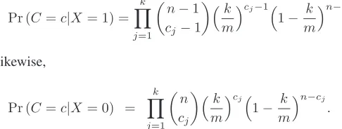
because by definition a Bloom filter always returns 1 for an element in the set S, i.e.Pr(BF= 1|x∈S) = 1. Likewise,
Pr(x /∈S|BF= 1) = 1−Pr(x∈S|BF= 1)
=Pr(BF= 1)−Pr(x∈S) Pr(BF= 1) .
ForBF= 1, letE1(x)denote the expected cost of a positive decision for an elementx, andE0(x)for a negative decision. Then,
E1(x) = Pr (x /∈S|BF= 1)·WF P
=Pr(BF= 1)−Pr(x∈S) Pr(BF= 1) ·WF P,
and
E0(x) = Pr (x∈S|BF= 1)·WF N = Pr(x∈S)
Pr(BF= 1)·WF N.
The Bloom paradox occurs when E1(x)> E0(x), i.e Pr(BF= 1)−Pr(x∈S)
Pr(BF= 1) ·WF P >
Pr(x∈S)
Pr(BF= 1)·WF N,
which can be rewritten as
Pr(BF= 1)>(α+ 1)·Pr(x∈S).
We use our model assumption that Pr(BF = 1) = (1/2)ln(2)·(m/n) if x /∈ S. Also, Pr(BF = 1) = 1 if x∈ S. Then, the left side of the last condition can be rewritten as
(1/2)ln(2)·(m/n)·Pr(x /∈S) + 1·Pr(x∈S), and we finally have
(1/2)ln(2)·(m/n)·(1−Pr(x∈S))> α·Pr(x∈S),
which provides the requested result.
B. Analysis of the Bloom Paradox
We now provide an illustration of the impact of various parameters on the Bloom paradox.
Figure 2(a) illustrates the probability that a Bloom filter is indeed correct when it indicates that an elementxis a member of the set. This probability,Pr (x∈S|BF= 1), depends on the
10−6 10−5 10−4 10−3 10−2 10−1 10−7
10−8 10−4 10−2 100
10−6
BF correctness probability
a priori set−membership probability fpr = 10−2 fpr = 10−3 fpr = 10−4 fpr = 10−5
(a) The Bloom filter correctness probability as a function of the a priori set-membership probability.
10−6 10−5 10−4 10−3 10−2 10−1 10−7
100−8 10 20 30 40 50
minimal m / n ratio
a priori set−membership probability
α = 0.1
α = 1
α = 10 α = 100
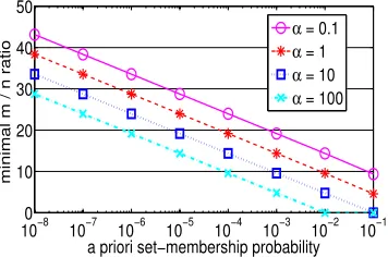
[image:4.612.101.284.57.177.2](b) Boundaries of the Bloom paradox: minimal number of bits-per-element for a Bloom filter to avoid the Bloom paradox, as a function of thea priori set-membership probability.
Fig. 2. Analysis of the Bloom paradox. (a) shows that a lower a priori probability makes the Bloom filter increasingly irrelevant, because the a posteriori membership probability after the Bloom filter is positive is also lower. This favors the Bloom paradox. (b) provides the exact borders of the region in which the Bloom paradox occurs as a function of the a priori probability, the Bloom filter load, and the relative weights of false-positive and false-negative errors.
instance, if Pr(x∈S) = 10−6 and the false positive rate is 10−3, the Bloom filter is correct w.p. Pr (x∈S|BF= 1) =
Pr(x∈S) Pr(BF=1) =
10−6
10−3·(1−10−6)+1·10−6 ≈10−6/10−3= 10−3.
Figure 2(b) plots the boundaries of the Bloom paradox. It presents the minimal bits-per-element ratio m/n needed to avoid the Bloom paradox, as a function of the a priori
probability, givenα= 0.1,1,10,100. For instance, ifα= 1, i.e. the costs of the two possible errors are equal, and the a priori probability isPr(x∈S) = 10−6, at least m/n= 28.7 memory bits per element are required to consider the Bloom filter and avoid the Bloom paradox. If this ratio is smaller, the Bloom paradox occurs, so we should return a negative answer for all the queries of x, independently of the answer of the Bloom filter.
C. Bloom Filter Improvements Against the Bloom Paradox
Based on the observation in Theorem 1, we suggest the two following improvements to Bloom filters, as illustrated in Figure 3:
Selective Bloom Filter Insertion—If the a priori proba-bility of an element x satisfies the Bloom paradox, we will not take the answer of the Bloom filter into account after the
query. Therefore,it is better not to even insert it in the Bloom filter, so as to reduce the load of the Bloom filter. Therefore, the final numbern∗ of inserted elements may satisfyn∗< n. Selective Bloom Filter Query—If thea prioriprobability of an elementxsatisfies the Bloom paradox, we do not want to take the answer of the Bloom filter into account, and therefore it is better to not even query it. Formally, if Pr(x ∈ S) < P0= (1 +α·2ln(2)·(m/n
∗)
)−1, wheren∗ is the final number
of inserted elements, then a negative answer should be returned for the queries ofx, regardless of the Bloom filter.
Each of these two improvements can be implemented inde-pendently. Implementing the Selective Bloom Filter Insertion alone yields fewer insertions and therefore a lower Bloom filter load, leading to a lower false positive probability. In turn, implementing the Selective Bloom Filter Query alone makes a regular Bloom filter more efficient by discarding useless query results for elements with low a priori probability. Finally, implementing both the Selective Bloom Filter Insertion and
Query results in the strongest improvement that combines the benefits of both approaches. All these approaches are further compared using simulations in Section VII.
Note that each of the two improvements requires knowing the a prioriprobabilities at different times (either during the insertion or during the query). Also, as expected, this approach may cause false negatives, since this may reduce the overall error cost.
D. Estimating thea PrioriProbability
Access patterns to caches tend to have the locality of reference property, i.e. it is more likely that recently-used data will be accessed again in the near future. Therefore, the
a priori probability distribution might be significantly non-uniform overU.
In such cases, we suggest to estimate thea prioriprobability by sampling arbitrary element queries and checking whether they belong to the cache. In practice, for 1% of element queries, we will check whether they belong to the cache, and use an exponentially-weighted moving average to approximate thea prioriprobability.
In addition, there might be several subsets of elements with clearly different a priori probabilities. For instance, packets originating from Class-A IP addresses might have distinct a priori probabilities from those with classes B and C. Then we will simply model thea prioriprobability as uniform over each class, and sample each class independently.
V. THEBLOOMPARADOX IN THECOUNTINGBLOOM
FILTER
A. The CBF-Based Membership Probability
[image:4.612.107.285.216.334.2](a) Selective Bloom Filter Insertion. Elements with low a prioriset-membership probability are not in-serted into the Bloom filter.
[image:5.612.278.557.62.153.2](b) Selective Bloom Filter Query. Elements with lowa prioriset-membership probability are not even queried, as shown in the first rectangle, and a negative answer is always returned for them no matter what the Bloom filter would have actually stated.
Fig. 3. Logical view of the Selective Bloom Filter implementation. Components that also appear in a regular Bloom filter are presented in gray. (a) shows a first possible improvement during insertion, where elements that satisfy the Bloom paradox are not even inserted into the Bloom filter. (b) displays a second possible improvement during query, where elements that satisfy the Bloom paradox are not even queried.
the element is inside that set. Finally, we prove a simple result that surprised us: to determine whether an element that hashes into kcounters falls under the Bloom paradox, we only need to comparethe product of these counterswith a threshold, and do not have to analyze a full combinatorial set of possibilities. For an element x∈U, we denote by Pr (x∈S|CBF)its membership probability inS, based on its CBF counter values. That is, on the values of the k counters with indices hj(x)
for j ∈ {1, . . . , k} pointed by the set of k hash functions
{h1, . . . , hk}. Let C = (C1, . . . , Ck) denote the k counter
indices of x, i.e. Cj = hj(x) for j ∈ {1, . . . , k}, and let
c= (c1, . . . , ck)denote the values of these counters.
Theorem 2: The CBF-based membership probability is
Pr (x∈S|CBF) =
mk·(Qk
j=1cj)·Pr(x∈S)
mk·(Qk
j=1cj)·Pr(x∈S) + (n·k)k·(1−Pr(x∈S))
.
Proof Outline: (The full proof can be found in [11].) Let
X be an indicator variable for the event x ∈ S such that
X = 1 iff x ∈ S. If cj = 0 for any j ∈ {1, . . . , k}, then
Pr (x∈S|CBF) = 0. Otherwise, we use the independency among the different sub-arrays of the CBF. If X = 1 then
x∈Sis one ofninserted elements. Thus,cj−1is the number
of times that the counterCj was accessed by the othern−1
elements in S. We now have that
Pr (C=c|X = 1) =
k
Y
j=1 n−1
cj−1
k
m
cj−1
1− k m
n−cj
.
Likewise,
Pr (C=c|X = 0) =
k
Y
j=1 n
cj
k
m
cj 1− k
m
n−cj
.
Putting all together using Bayes’ rule yields the result. Directly from the last theorem we can deduce the following corollary.
Fig. 4. Logical view of the Selective Counting Bloom Filter implementation. Components that also appear in a regular CBF are presented in gray. Mem-bership probability is calculated based on the counters product. A negative answer is returned for elements with low calculated membership probability.
Corollary 3: For an element x∈U, the CBF-based mem-bership probability Pr (x∈S|CBF) is an increasing func-tion of the product of the k counters pointed by hi(x) for
i∈ {1, . . . , k}.
B. Optimal Decision Policy for a Minimal Cost
We now suggest an optimal decision policy for the query of an element x ∈ U in a CBF. This policy relies on its CBF-based membership probability, which was expressed in Theorem 2 as a function of the product of its counter values.
Theorem 4: An optimal decision policy for the CBF is to be positive iff
Pr (x∈S|CBF)≥ 1 α+ 1.
Proof Outline: (The full proof can be found in [11].) We again compare the expected costs E1(x) and E0(x) of a positive and negative decision and show thatE1(x)≤E0(x) when Pr (x∈S|CBF)≥ α1+1.
Figure 4 illustrates the improved logical process of a query of an elementxin the Selective Counting Bloom Filter. It is similar to the query process of the Selective Bloom Filter that was presented in Figure 3(b). Here, the product of counters is used to calculate the membership probability.
[image:5.612.323.558.253.336.2] [image:5.612.55.298.585.677.2]VI. A MEMORYLOWERBOUND ON ADATASTRUCTURE
WITHFALSEPOSITIVES ANDFALSENEGATIVES A. Related Work
As we have noticed so far, the suggested schemes may yield false positives as well as false negatives. In order to examine the efficiency of the solution, we would like to present lower bounds on the memory required to represent a set of a given size with limited false-positive and false-negative rates. Let
S ⊆U be the represented set ofnelements from a universe of size |U| =N. Likewise, letǫ,δ denote the upper bounds of the false-positive and false-negative rates, respectively.
Carter et al. suggested in [12] a lower bound on the number of bits m required to represent such a set S without false negatives. Any string that representsScan accept at mostn+
ǫ(N−n)elements. Thus, any stringscan represent correctly at most n+ǫ(nN−n)
sets. In order to represent all the possible sets by strings of length m, we have:
2m
n+ǫ(N −n)
n
≥
N
n
,
or alternatively (forN ≫n) the entropy lower bound is
m≥log2
N n
n+ǫ(N−n)
n
!
≈nlog2(1/ǫ).
This entropy lower bound was generalized in [13] for the case that both false positives and false negatives are allowed in the concept of limited-error dictionaries. To do so, they calculate again the number of sets that can be represented correctly by the same string ofm bits.
B. Improved Memory Lower Bound
Although the last mentioned bound can also apply to Bloom filters, we would like to present a more accurate analysis of this case without some of their assumptions and approximations.
To do so, we first present Lemma 1, which helps us then prove Theorem 5. For space reasons, the proof of this lemma can be found in [11].
Lemma 1: The number of sets of size nthat can be repre-sented with limited false positive and false negative rates ofǫ
andδ, by a string that accepts exactly aelements is
Xa =
min(n,a) X
i=max(a−ǫ(N−n),(1−δ)n) a
i
N−a
n−i
.
Based on the lemma we can deduce the following theorem.
Theorem 5: The numberm of bits in a string representing a set S with the requested error rates from above satisfies
m≥log2 N
n
/
max
a∈RXa
!
.
Proof: As in the calculation of the previous bound, all the possible Nn
sets must be represented correctly by one of the 2mstrings ofmbits. Since each string represents at most
maxa∈R(Xa)sets, the result follows.
VII. SIMULATIONS A. Bloom Filter Simulations
Table II compares the false positive rate (fpr), false negative rate (fnr) and the total cost for the Bloom Filter (BF) [1], Generalized Bloom Filter (GBF) [7], Retouched Bloom Filter (RBF) [6] and the suggested Selective Bloom Filter with its three variants.
We assume a set S composed of 256 elements from each of 13 types of elements, such that n = |S| = 28 ·13 = 256·13 = 3328. Each subset of 256 elements are selected homogenously among sets of sizes 211,212, ...,223. Thus, for
i∈[1,13]an element of thei-th type is member ofS witha prioriset-membership probability of2−(i+2)andN =|U|= P13
i=12i+10 = 16775168. The numbers of bits per element (bpe) are4,6,8and10such thatm=n· bpe.
As usual, the false positive rate (fpr) is calculated among theN−nelements ofU\S and the false negative rate (fnr) is calculated among thenmembers ofS. In the calculation of the total cost, we assume thatWF P = 1andWF N =αsuch
that the cost equals(N−n)· fpr +n·fnr·α. The results are presented for the valuesα= 100andα= 5, which illustrate two possible scenarios for the ratio of the two error costs. In the Bloom Filter and in the three variants of the Selective Bloom Filter we usek≈ln(2)·(m/n)hash functions. In the Generalized Bloom Filter we use k1 = k hash functions to select bits to be set. Likewise, the number of functions used to select bits to reset, k0∈[1, k1−1], was chosen such that the total cost is minimized. For the Retouched Bloom Filter we used theRatio Selectionas the clearing mechanism. In this heuristic, shown to be the best scheme in [6], the bits to be reset are selected, such that the ratio of the additional false negatives and the cleared false positives is minimized.
We first note that when thea prioriset-membership proba-bilities are available in the insertion process as well as in the query process, the Selective Bloom Filter always improves the total cost achieved in BF, GBF and RBF, even whenα= 100 and therefore the cost of a false negative is very high. For instance, when the probabilities are used in the insertion as well as in the query, with a memory of 4 bits per element (and α = 100) the total cost is 1.78e5 in comparison with 2.46e6, 6.37e5 and 3.32e5 in BF, GBF and RBF respectively, i.e. a relative reduction of 92.76%, 72.04%, 46.46%.
If α = 5, the cost of a false negative is relatively small. As a result, optimizing the tradeoff of fpr vs. fnr results in an (fpr,fnr) pair of (1.87e-4, 5.38e-1) instead of (3.08e-3, 3.80e-1) forα= 100. That is, as expected, the fpr is smaller and the fnr is larger when the relative cost of fnr is smaller. Ifα= 5, the cost is 1.21e4 instead of 2.46e6 in BF. This is a significant improvement by more than two orders of magnitude.
(a)α= 100
Bloom Filter Generalized Bloom Filter Retouched Bloom Filter
bpe m fpr fnr cost fpr fnr cost fpr fnr cost
4 13312 1.47e-1 0.00 2.46e6 2.52e-2 6.46e-1 6.37e5 0.00 1.00 3.32e5
6 19968 5.63e-2 0.00 9.44e5 5.06e-3 7.35e-1 3.29e5 0.00 1.00 3.32e5
8 26624 2.17e-2 0.00 3.64e5 3.09e-4 8.65e-1 2.93e5 3e-6 1.00 3.32e5
10 33280 8.24e-3 0.00 1.38e5 1.35e-4 8.44e-1 2.83e5 8.87e-3 0.00 1.49e5
Selective Bloom Filter Selective Bloom Filter Selective Bloom Filter (Only Insertion) (Only Query) (Insertion & Query)
bpe m fpr fnr cost fpr fnr cost fpr fnr cost
4 13312 4.94e-2 3.64e-1 9.49e5 2.20e-3 4.62e-1 1.90e5 3.08e-3 3.80e-1 1.78e5 6 19968 2.40e-2 2.24e-1 4.78e5 1.60e-3 3.85e-1 1.55e5 3.00e-3 2.31e-1 1.27e5 8 26624 9.28e-3 1.51e-1 2.06e5 2.29e-3 2.31e-1 1.15e5 2.31e-3 1.54e-1 9.00e4 10 33280 5.39e-3 7.64e-2 1.16e5 1.99e-3 1.54e-1 8.45e4 2.69e-3 7.69e-2 7.08e4
(b)α= 5
Bloom Filter Generalized Bloom Filter Retouched Bloom Filter
bpe m fpr fnr cost fpr fnr cost fpr fnr cost
4 13312 1.47e-1 0.00 2.46e6 2.53e-2 6.43e-1 4.34e5 0.00 1.00 1.66e4
6 19968 5.66e-2 0.00 9.50e5 5.06e-3 7.34e-1 9.70e4 0.00 1.00 1.66e4
8 26624 2.17e-2 0.00 3.64e5 3.04e-4 8.65e-1 1.95e4 0.00 1.00 1.66e4
10 33280 8.23e-3 0.00 1.38e5 1.33e-4 8.43e-1 1.63e4 0.00 1.00 1.66e4
Selective Bloom Filter Selective Bloom Filter Selective Bloom Filter (Only Insertion) (Only Query) (Insertion & Query)
bpe m fpr fnr cost fpr fnr cost fpr fnr cost
4 13312 2.47e-2 5.24e-1 4.23e5 1.16e-4 7.69e-1 1.47e4 1.87e-4 5.38e-1 1.21e4 6 19968 7.90e-3 4.56e-1 1.40e5 9.1e-5 6.92e-1 1.31e4 2.44e-4 4.61e-1 1.18e4 8 26624 2.22e-3 3.83e-1 4.37e4 6.8e-5 6.15e-1 1.14e4 1.39e-4 3.84e-1 8.73e3 10 33280 1.21e-3 3.07e-1 2.53e4 1.22e-4 4.62e-1 9.72e3 1.52e-4 3.08e-1 7.67e3
TABLE II
COMPARISON OF FALSE POSITIVE RATE(FPR),FALSE NEGATIVE RATE(FNR)AND THE TOTAL COST FORBLOOMFILTER, GENERALIZEDBLOOMFILTER, RETOUCHEDBLOOMFILTER AND THE SUGGESTEDSELECTIVEBLOOMFILTER WITH THREE VARIANTS. IN THE FIRST,THEa prioriSET-MEMBERSHIP PROBABILITY IS USED ONLY DURING THE INSERTION OF THE ELEMENTS,WHILE IN THE SECOND VARIANT IT IS USED ONLY IN THE QUERY PROCESS AND IN THE THIRD ONE IT IS USED IN BOTH OF THEM. THE TOTAL NUMBER OF INSERTED ELEMENTS ISn= 256·13 = 3328WITHa prioriSET-MEMBERSHIP
PROBABILITIES OF2−3
,2−4
, ...,2−15
AND|U|= 16775168.
fact that in our experiment, the set U\S is much larger than the setS itself. Thus, the effect of avoiding the false positives of elements with smaller a prioriset-membership probability during the query is larger than the effect achieved by avoiding the insertion of elements with such probabilities.
B. Counting Bloom Filter Simulations
In this section we conduct experiments on CBFs. We first examine the CBF-based membership probability in compari-son with Theorem 2.
Then, we try to use these probabilities to further reduce the expected cost of a query.
The setS is defined exactly as in the previous simulation. It again includesn= 13·256 = 3328elements of13types with
a prioriprobabilities of 2−3,2−4, ...,2−15. Here, since CBFs with four bits per entry are used, we consider bpe values of 16,24,32and40.
Figure 5 displays the membership probability based on the values of the k = 6 counters. According to Theorem 2, the
probability can be described as a function of the product of these k counters. The figure presents the results for up to a product of 100, since larger products were encountered in the simulations with a negligible probability. The simulated probabilities for the most common values are compared with the theory. The dependency in the a priori set-membership probability is demonstrated again. For instance, if the product is 8, the observed probabilities are 0.90594,0.68504 and 0.34679for thea prioriprobabilities2−3,2−5,2−7. Likewise, to obtain a membership probability of at least0.8, the minimal required products are5,23and91, respectively.
Counting Bloom Filter Selective Counting Bloom Filter (Only Query)
bpe m fpr fnr cost fpr fnr cost
16 13312 1.47e-1 0.00 2.46e6 8.95e-5 7.65e-1 1.42e4
24 19968 5.61e-2 0.00 9.40e5 9.59e-5 6.57e-1 1.25e4
32 26624 2.16e-2 0.00 3.61e5 9.42e-5 5.35e-1 1.05e4
[image:8.612.366.541.53.180.2]40 33280 8.20e-3 0.00 1.37e5 1.01e-4 4.16e-1 8.61e3
TABLE III
SIMULATION RESULTS FORCOUNTINGBLOOMFILTERS WITHα= 5.
SIMULATION PARAMETERS ARE THE SAME AS INTABLEII.
same as that of the Bloom filter. This is because its regular query policy cannot contribute to reduce the false positive rate. Our suggested policy for the decision helps to reduce the total cost by at most 99.42%. By comparing the query policy of the Selective CBF to the results of the suggested query policy in the Selective Bloom Filter (presented in Table III), we can see an additional improvement of up to 11.43%. This reduction in the total cost is due to the more accurate calculation of the membership probability based on the information on the exact values of the counters. Such information is not available in the Selective Bloom Filter.
C. Trace-Driven Simulations
We now want to explore the tradeoff of the false positive rate and the false negative rate in the Selective CBF. To do so, we conduct experiments using real-life traces recorded on a single direction of an OC192 backbone link [14]. We used a 64-bit mix hash function [15] to implement the requested hash functions. The hash functions are calculated based on the 5-tuple (Source IP, Destination IP, Source Port, Destination Port, Protocol).
The Selective CBF represents here, using 30 bits per el-ement and 4 bits per counter, a set of n = 210 different tuples that we encounter in a short period of 3614 µs. Our queries are based on N = 220 tuples (that includes the first n) that were encountered later on during a longer time interval. This yields ana prioriset-membership probability of
n/N = 210/220= 2−10.
Figure 6(a) illustrates this tradeoff. First, the solid line presents the tradeoff obtained by Theorem 5. We remind that this theorem is general and talks about the length in bits of a general representing binary string. However, in order to have a fair comparison with the Selective CBF and to compare apples to apples (i.e. counters to counters), in the calculation of this curve, we assume that each string entry has a width of 4 bits, the typical number of counter size in CBFs. Using binary search, we found for each value of the false negative rateδ, a maximal value of the false positive rateǫ, that still holds the memory constraint according to the theorem. For instance, if
δ= 0.001(i.e. at most⌊δ·n⌋= 1out ofnare not accepted by the representing string), we found a maximal false positive rate of ǫ= 0.004981 (and at most ⌊ǫ(N−n)⌋= 5217 elements outside the set are accepted by the string). Ifδ= 0.0316, then
ǫ drops to0.00360.
0 20 40 60 80 100
0 0.2 0.4 0.6 0.8 1
membership probability
counters product
[image:8.612.51.312.58.143.2]P = 2−3 (theory) P = 2−3 (simulation) P = 2−5 (theory) P = 2−5 (simulation) P = 2−7 (theory) P = 2−7 (simulation)
Fig. 5. CBF-based membership probability for elements witha priori set-membership probabilityP = Pr(x∈S). The probability is based onk=6 counter valuesand compared with Theorem 2.
The three dashed lines draw the tradeoff achieved using the Selective CBF with the k= 4,5and6 hash functions. Three points are located on the y-axis. They present, of course, the typical false positive rate of the CBF where no false negatives are allowed. The rates are0.03086,0.02850,0.02908, respec-tively and the minimum is achieved fork= 5≈30/4·log(2). Thus, if WF N is large enough and α → ∞, the optimal
number of hash functions isk= 5.
We earlier showed that the membership probability is an increasing function of the product of thek counters. In each of these three lines, each point illustrates a different threshold of the counters product such that a negative answer is returned only if the product is smaller than the threshold. As explained in Section V, in order to minimize the expected cost, each value ofαcan be translated to a probability threshold of α1+1 by Theorem 4 and later on also to a product threshold. For instance, forα= 2.4, the probability threshold is α+11 = 1034. Fork = 5, the product threshold is 6 and the obtained false positive and false negative rates are 0.00746 and 0.39258, re-spectively. However, lower error rates of 0.00739 and 0.34766 can be obtained fork= 6with the product threshold10. Thus, for suchα, for instance, the optimal number of hash functions is not the typical number of hash functions in a CBF.
Figure 6(b) compares the total cost of queries of the CBF and the Selective CBF in this simulation as a function ofα. We again assume 30 bits per element and k= 5 hash functions. Since the CBF does not allow any false negatives, its total cost is constant and equals the number of obtained false positives
ǫ(N−n) = 29856. For small values ofα, such thatα= 1and
(a) Tradeoff of false positive rate vs. false negative rate for 30 bits per element.
(b) Total cost ofN queries in the CBF and the Selective CBF. The cost of a false positive is1, and the cost of a false negative isα. Since the CBF does not allow any false negatives, its cost is constant and does not depend onα. For smaller values of α, the improvement of the Selective CBF is more significant.
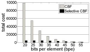
[image:9.612.55.207.59.146.2](c) Total cost ofN queries in the CBF and the Selective CBF as a function of the number of bits per element (bpe). The cost of a false positive is 1, and the cost of a false negative isα= 5. For smaller values of bpe, the false positive rate of the CBF is larger. The probability that its positive indication is correct is lower, and the improvement of the Selective CBF is more significant.
Fig. 6. Trace-Driven Simulations
cost is approximately reduced by an order of magnitude. Figure 6(c) compares the total cost of queries of the CBF and the Selective CBF in the simulation above, as a function of the number of bits per element (bpe). For each value of bpe, the optimal number of hash functions of the CBF is used (in both schemes) and the results are presented for α= 5. If less bits per element are used, the false positive rate of the CBF is larger. The probability that its positive indication is correct is lower, and the improvement of the Selective CBF is more significant. Likewise, the tradeoff in the Selective CBF is improved using more bits per element, and thus also its total cost. In all cases, the Selective CBF achieves a lower total cost than the CBF. For instance, if bpe=20, the cost of the CBF is reduced from98561by 94.80% to5122. Ifbpe= 50, the costs are 2690and 1876, respectively. In this case, since the false positive rate of the CBF is smaller, the relative improvement drops to 30.26%.
VIII. CONCLUSION
In this paper, we introduced theBloom paradoxand showed that in some cases, it is better to return a negative answer to a query of an element, even if the Bloom filter or the CBF indicate its membership. We developed lower bounds on the a prioriset-membership probability of an element that is required for the relevancy of the Bloom filter in its queries. We also showed that the exact values of the CBF counters can be easily used to calculate the set-membership probability. Last, we showed that our schemes significantly improve the average query cost.
IX. ACKNOWLEDGMENT
This work was partly supported by the European Research Council Starting Grant No. 210389, by the Jacobs-Qualcomm fellowship, by an Intel graduate fellowship, by a Gutwirth Memorial fellowship, by an Intel research grant on Hetero-geneous Computing, and by the Hasso Plattner Center for Scalable Computing.
REFERENCES
[1] B. Bloom, “Space/time tradeoffs in hash coding with allowable errors,” Communications of the ACM, vol. 13, no. 7, 1970.
[2] L. Fan, P. Cao, J. M. Almeida, and A. Z. Broder, “Summary cache: a scalable wide-area web cache sharing protocol,” IEEE/ACM Trans. on Networking, vol. 8, no. 3, 2000.
[3] F. Bonomi, M. Mitzenmacher, R. Panigrahy, S. Singh, and G. Varghese, “An improved construction for counting Bloom filters,” inESA, 2006. [4] H. Song, F. Hao, M. S. Kodialam, and T. V. Lakshman, “IPv6 lookups
using distributed and load balanced Bloom filters for 100gbps core router line cards,” inIEEE Infocom, 2009.
[5] O. Rottenstreich, Y. Kanizo, and I. Keslassy, “The variable-increment counting Bloom filter,” inIEEE Infocom, 2012.
[6] B. Donnet, B. Baynat, and T. Friedman, “Retouched Bloom filters: allowing networked applications to trade off selected false positives against false negatives,” inACM CoNEXT, 2006.
[7] R. P. Laufer, P. B. Velloso, and O. C. M. B. Duarte, “A generalized Bloom filter to secure distributed network applications,” Computer Networks, vol. 55, no. 8, 2011.
[8] W. Thompson and E. Shumann, “Interpretation of statistical evidence in criminal trials: The prosecutor’s fallacy and the defense attorney’s fallacy,”Law and Human Behavior, vol. 1, no. 3, 1987.
[9] H. L. Vacher, “Quantitative literacy - drug testing, cancer screening, and the identification of igneous rocks,”Journal of Geoscience Education, 2003.
[10] P. Beauchemin, G. Brassard, C. Crepeau, and C. Goutier, “Two obser-vations on probabilistic primality testing,” inCrypto’, 1986.
[11] O. Rottenstreich and I. Keslassy, “The Bloom paradox: When not to use a Bloom filter?” Comnet, Technion, Israel, Tech. Rep. TR11-06, 2011. [Online]. Available: http://webee.technion.ac.il/∼isaac/papers.html [12] L. Carter, R. W. Floyd, J. Gill, G. Markowsky, and M. N. Wegman,
“Exact and approximate membership testers,” inACM STOC, 1978. [13] R. Pagh and F. F. Rodler, “Lossy dictionaries,” inESA, 2001. [14] C. Shannon, E. Aben, K. Claffy, and D. E. Andersen, “CAIDA
anonymized 2008 Internet trace equinix-chicago 2008-03-19 19:00-20:00 UTC (DITL) (collection),” http://imdc.datcat.org/collection/. [15] T. Wang, “Integer hash function,” http://www.concentric.net/∼Ttwang/
tech/inthash.htm.
[16] S. Iyer, R. R. Kompella, and N. McKeown, “Designing packet buffers for router linecards,” IEEE/ACM Trans. on Networking, vol. 16, no. 3, pp. 705–717, 2008.
[image:9.612.406.557.60.147.2]