Fourth Order Variational Multiplicative Noise Removal Model

(1)

Fourth Order Variational Multiplicative Noise

Removal Model

Noor Badshah

Mushtaq Ahmad Khan

Asmat Ullah

Abstract - Multiplicative noise removal based on total variation (TV) regularization has been widely re-searched in image science. In multiplicative noise problems, original image is multiplied by a noise rather than added to the original image. Usually, the logarithmic amplification transforms the multiplicative noise model into the classical additive noise problem. This additive noise problem is then solved by ROF [23] model. In this paper we propose a model for multiplicative noise based on Euler’s Elastica model for additive noise [8]. Numerical examples demonstrate that the proposed algorithm is able to preserve small image details while the noise in the homogeneous regions is removed sufficiently. As a consequence, our method yields better denoised results than those of the current state of the art methods with respect to the SNR values.

Keywords - Speckle, Synthetic Aperture Radar (SAR), Total Variation (TV), Additive Operating Splitting (AOS)

I. INTRODUCTION

The standard statistical models of coherent imaging systems, such as synthetic aperture radar/sonar (SAR/SAS), ultrasound imaging, and laser imaging, are supported on multiplicative noise mechanisms. Speckle is a phenomenon whose configuration is random and it yields random fluctuation of the complex reflectivity. The statistical properties of speckle have been widely studied and there is a large body of literature [10, 16]. Assuming no strong specular reflectors and a large number of randomly distributed scatterers in each resolution cell (relative to the carrier wavelength), the squared amplitude (intensity) of the complex reflectivity is exponentially distributed [16]. The term multiplicative noise is clear from the following observation: an exponential random variable can be written as the product of its mean value (parameter of interest) by an exponential variable of unit mean (noise). The scenario just described, known as fully developed speckle, leads to observed intensity images with a characteristic granular appearance due to the very low signal to noise ratio (SNR). Notice that the SNR, defined as the ratio between the squared intensity mean and the intensity variance, is equal to one.

Image denoising is an inverse problem widely studied in signal and image processing fields. The problem includes additive noise removal and multiplicative noise removal. In this paper, we will mainly discuss the multiplicative noise removal problem. Multiplicative noise removal problem can be modeled in the following way

z(x, y) = g(x, y)v(x, y), (1)

where z is the observed image, g is the original image and v is the noise which follows a Gamma law with mean one.

II. PREVIOUS

WORK

In many papers, multiplicative noise models have been discussed. One of the method is local linear minimum mean square approaches [13, 12], anisotropic diffusion methods [15, 24], These models are based on statistical information of images and noise, so we will not discuss these models in detail as in this paper our main focus is on variational models.

In recent years, variational methods have got great success in reducing the multiplicative noise owing to the use of total variation (TV) and nonlocal total variation (NLTV) regularizations. The TV based variational models for multiplicative noise removal have been proposed in many literatures like Rudin et al.[17], Aubert and Aujol [1], Shi and Osher [19], Huang et al. [11], Steidle and Teuber [20], Li et al. [14], etc. The variational based NLTV models [10] have also been widely applied in image restoration [25], [20]. Steidl and Teuber [20] employed the NLTV as a regularizer to recover the multiplicative noisy images. Since the NLTV norm uses the relevant image patches,that’swhy it gives very good qualitative results.

The elastica model [8] minimizing the Euler elastica energy for image inpainting problem is the following











2

/ min ( )

(2) 2

p u u

D

J u a b dxdy

u z dxdx

 



  

 



where a and b are arbitrary positive constants, λ >0 is a penalty parameter, p = 2 is usually chosen, u = u(x, y) is the true image to be restored and . u

u



  

 is the

curvature.

The virtue of equation (2) is that the regularization using the Euler elastic energy penalizes the integral of the square of the curvature along edges instead of only penalizing the length of edges as the TV model (if taking b = 0) does [7]. Motivated from the performance of Euler elastica model in image inpainting and denoising, in this paper we would use this idea towards image multiplicative denoising.

III. LI-LI

HUANG

MODEL

(M1)

(2)

ˆ _{arg min ( )}_E _J_{( )} _{log( )} z _dx_, ₍₃₎ 

   



 

   _  _



 



where

1 2

( ) D (4)

J



D dxdy



dxdy



 

 



 



the regularization term in which the first term is Based on TV and the second term is Weberized TV which is given by



log( )



D

TV dxdy



  





Thus they consider the following minimization problem

1 2

ˆ _{arg min ( )}

log( ) (5)

E

z dx



  



 





     

 

 _   _



 



Here z > 0 in L∞(Ω) is the given data in the model.The first two terms are the regularization terms, while the third one is the nonconvex data fidelity term following the MAP estimator for multiplicative Gamma noise, μ1, μ2 are regularization parameters.

Minimization of the functional (5) leads to the following Euler-Lagrange equation

1 2

2 2

. z 0



 

         

_ _{ } _ __ 

 

  __   __

in



0

n

_ 

on the. (6)

Since ϕ > 0, so the Euler Lagrange equation of the

minimization can be written as





2 2

1 2

( ) 0

z



 

  

 

_   

       

 

in



0 n









on the



. (7)

Define

 



1 2



1 ,

    

    

  _{then equation (7) can be} written as





2

( ) . 0

E z



 



 

   _ _    

   

 

 _in_Ω.

(8) with Newmann boundary conditions. Fixed point iterations are used to solve this equation (8)

 

L

   



z

(9)

Where L(φ) is the linear operator whose action on the function q is given as

 

₂ ( )

L q div q



 



 

   _ _  

   

 

 ₍₁₀₎

The finite difference method is communally used for

accurate finite difference method as follow [21],

 





 





1, , , 1 ,

2 2

, , , ,

2 2

, , , ,

,

( ; (

x i j i j y i j i j

x i j x i j y i j y i j

y i j y i j x i j x i j

D D

D D m D D



 

  

   

  _  _   _  _

 

    _   _ 

 

    _   _ 

Where m[a, b] = (sign(a) + sign(b))/2.min(|a|, |b|). Here we take the space step size by h = 1,ξ > 0.

These schemes yields approximate f o r m (10)

( )

(

x

) (

(

y

)

( )

x y

y y

D q

L

q

D

q

D u

 

 

 

 



  



₍₁₁₎

Where L is the matrix operator, wh i c h are symmetric, positive definite and sparse

IV. CHEN

SHENG

MODEL

(M2)

Let us consider equation (1), by applying the logarithmic amplification, the equation (1) will transform into classical additive noise form [18]:

log(z(x, y)) = log((g(x, y)) + log((v(x, y)). (12)

The above expression can be rewritten

f(x, y) =φ(x, y) +η(x, y), (13)

where f (x, y) is given noisy image having additive gaussian type noiseη(x, y) and φ(x, y) is the noise free image, where (x, y)²R2. The minimization of the above equation (13) by ROF [23] is given as

 

1





2

min ( ) ,

2

E R f dxdy

 

    



 



  (14)

with R( ) dxdy 

 



 is the regularizer term.

Minimization o f the above functional gives the following EulerLagrange’s equation [23]





2

. z 0



 



 

_ _    

   

 

in



0 n



_





on the



. (15)





2

( ) . 0

E z



 



 

   _ _    

   

 

inΩ. (16)

with Newmann boundary condition on the domain of the image. The corresponding time marching equation from (15) is





2 2 2 2 0

y x

x y x y

z

t x y

 _   _ 

_  _ __  _ __{   } _

   

  _ _{  } _  _ _{  } _

   

(17)

Numerical solution of the differential equation given in (16) can be found in similar lines as done in [23], for given u(x, y, 0), t > 0, x,

y



R

and also

n





= 0 on

(3)

( ,

ih jh

)





have been chosen initially. In this case ϕ has mean 0 and L2 norm one. The numerical approximation for (17) is given as





















1 2 2 2 2 0 ( ( ), ( ( ), , ( , ) k x ij k k

ij ij x

k k k

x ij y ij y ij

k y ij y

k k k

y ij x ij x ij k K ij D t D h

D m D D

D D

D m D D

tc ih jh

                   _        _ _ _ _ _ _  _ _               _ _ _ _   _     

for i,j = 1, 2, 3 …. M with boundary conditions

  

₀_j ₁_j

,

1

,

0 1

Mj Mj i iM iM

  

    

where as



1



x i j ij

D



    

_ and

D

_y

    



_ij_₁ _ij



.

V. THE

PROPOSED

MODEL

(M3)

As form the minimization approach (14) we have the regularizer term



2



( )

,

R

a b



D dxdy



 

_





Which is the curvature based regularization instead of TV norm. Where a and b are the parameters and

 

x y, .

    

 is the curvature, so (14) becomes









2

ˆ _{arg min ( )}

(18) 2

E a b dxdy

f dxdy               



Minimization of the above functional leads to the following Euler Lagrange’s equation [9]

  

.V f



0 (19)

      

Where



2







3 2

. b

V a b  

 _                   

With boundary conditions 0

x

_

 and



2



0 a b v      .

Where



is the normal vector and

 

 is the corresponding tangent vector i.e.



,



,



,



n    x y t      y x

Numerical solution of the differential equation given in (19) can be found in similar lines as done in [6]. We discretize (19) as follow.

1 2

.V V V .

x y

 

  

 

1 1 2 2

1 1 1 1

, , , ,

2 2 2 2

, .

i j i j i j i j i j

V V V V

V h h                         

Here we approximate 1₁ , 2 i j V  and 1 1 , 2 i j V  .

Curvature term. These are approximated by min-mode

of two adjacent whole pixels.









1 1, ,

, 2

1 , 1,

, 2

min mode ,

i j i j i j

i j i j i j              

Where min-mode



_,

 

sgn sgn



_min



_,



2

m n

m n  _  _ m n

 

.

Partial derivatives in x . By the central difference of

two adjacent whole

















1 1, , 1 , 1,

, ,

2 2

1, 1, 1, , ,

2

1 1

,

1

,

i j i j i j i j

i j i j

i j i j i j i j i j x x h h x h                 _ _     _ _                











 



1_, , _, 1, _1,

2

2 2 ₂

1, 1, , 1 , 1

, 1 . 1 4 2

i j _{i j} i j _i _j i j

i j i j i j i j i j x h h  _                         

Where



0

.

Partial derivatives in y. By min-mode of ∂y, s at two

adjacent whole points,









1 1, 1 1, 1

, 2

, 1 , 1

1

m in m o d e ,

2

1 2

i j i j i j

i j i j

y h h          _      _      _       _ 









1 , 1 , 1

, 2

1, 1 1, 1 1

minmode ,

2

1 2

i j i j i j

i j i j

y h h          _    _ _ _           _ 

















1 , 2

, 1 _, ₁ , 1 _, ₁

1, 1 _1, ₁ 1, 1 _1, ₁ min mode , with 1

2 1 2

y _i _j

i j _{i j} i j _{i j}

i j _i _j i j _i _j

m n m n   _  _   _ _   _ _                  Also, 2 2

1 ₁ ₁

, _, _,

2 ₂ ₂

i j x _i_ _j y _{i j}_ 

               _ _   _ _   _ _  _ _     2 2

1 ₁ ₁

, _, _,

2 ₂ ₂

i j x _i_ _j y _{i j}_ 

(4)

By similar way we can find the approximations

for 2 ₁

, 2

i j

V

 and

2 1 ,

2

i j

V

 with Neumann boundary

conditions

,0 ,1, , 1 , , 0, 1, , 1, , .

i i i n i n j j m j m j

           

VI. EXPERIMENTAL

RESULTS

Here we take some experimentionl results on different images by the proposed model M3 and models M1 and M2 which show that proposed model M3 is more accurate and efficient than that of models M1 and M2.

The following are some noisy images for the compression of the models M1 and M2 and the proposed model M3.

Fig.1. The noisy images: (a) Noisy“Lena”image with L= 1.5, (b) Noisy“Camera man” image with L= 1.7, (c) Artificial synthetic image with L= 1.9, (d) Artificial synthetic image with L= 2.5

(a) Denoised image by M1

(b) Denoised image by M2

(c) Denoised image by M3 Fig.2. The restored “lena” images: (a) Denoised image by model M1, (b) Denoised image by model M2, (c) Denoise Image by proposed model M3

(a) Restored image using M1

(b) Restored image using M2

(c) Restored image using M3 Fig.3. The restored “Cameraman” images: (a) Denoised image by model M1, (b) De- noised image by model M2, (c) Denoise Image by proposed model M3

(a) Restored image using M1

(b) Restored image using M2

(c) Restored image using M3 Fig.4. Restoration of an artificial synthetic image: (a) Denoised image by model M1, (b) Denoised image by model M2, (c) Denoise Image by proposed model M3

(a) Denoised image by M1

(b) Denoised image by M2

(c) Denoised image by M3 Fig.5. Restoration of an artificial synthetic image: (a) Denoised image by model M1, (b) Denoised image by model M2, (c) Denoise Image by proposed model M3

In Fig. 2, M1, M2 and M2 are applied on a real Lena image, it can be seen that the results from M3 are of better quality than M1 and M2. In Fig. 2(a), results obtained by applying M1 and in Fig 2(b) results obtained by applying M2 and Fig 2(c) our model M3 is applied. Parameters used are µ1 = 0.05, µ2 = 7 andλ= 8 and a = 0.005, b = 1e−5,λ= 5 respectively . In Fig. 3 M1, M2 and M3 are tested on a real cameraman image. Fig. 3(a) results with M1 is given and in Fig. 3(b) restoration o f image using M2 is presented with µ1 = 2,

µ2 = 3, andλ = 6.5. In this case performance of our

model M3 is justified as well with parameters a = 0.005, b = 1e−3,λ= 7 respectively.

In Fig. 4 all the three methods are implemented on an artificial image and can be seen that our method M3 performed very well than M1 and M2. In Fig. 4(a) a noisy synthetic image which is denoised by M1, in Fig. 4(b) also denoised by M2 and in Fig. 4(c) also denoised by our proposed method wi th parameters µ1 = 0.05,

µ2 = 7,andλ = 6.5 and a = .05, b = 1e−5,λ = 8. In

Fig. 5 all the three methods are tested on another artificial image with the following parameters µ1 = 0.7, µ2 = 1 and = 5.8 and a = 0.01, b = 1e−3,λ= 8.

VII. PEAK

SIGNAL TO

NOISE

RATIO

(PSNR)

We also measure the quality of restoration of the restored Image by peak signal -to-noise ratio (PSNR) of the three models as follow;

2

max{ *}

10 log

M

N

u

PSNR



_





(5)

size of the image, respectively.

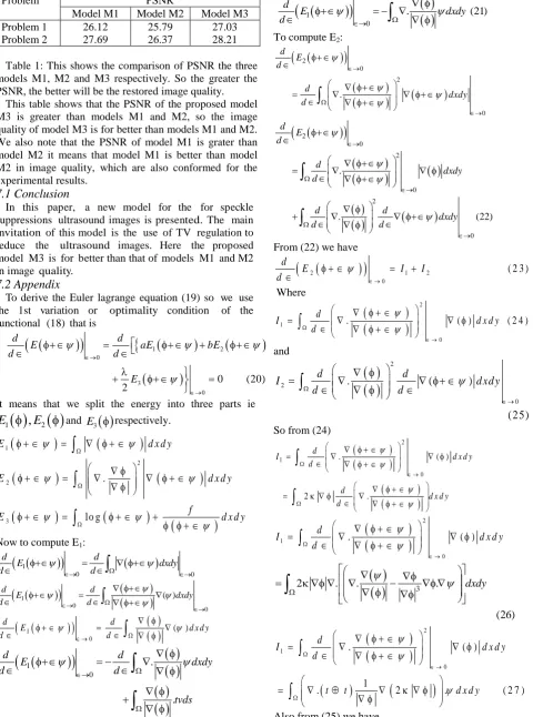
Problem PSNR

Model M1 Model M2 Model M3 Problem 1 Problem 2 26.12 27.69 25.79 26.37 27.03 28.21 Table 1: This shows the comparison of PSNR the three models M1, M2 and M3 respectively. So the greater the PSNR, the better will be the restored image quality.

This table shows that the PSNR of the proposed model M3 is greater than models M1 and M2, so the image quality of model M3 is for better than models M1 and M2. We also note that the PSNR of model M1 is grater than model M2 it means that model M1 is better than model M2 in image quality, which are also conformed for the experimental results.

7.1 Conclusion

In this paper, a new model for the for speckle suppressions ultrasound images is presented. The main invitation of this model is the use of TV regulation to reduce the ultrasound images. Here the proposed model M3 is for better than that of models M1 and M2 in image quality.

7.2 Appendix

To derive the Euler lagrange equation (19) so we use the 1st variation or optimality condition of the functional (18) that is























1 2 0 3 0 0 (20) 2 d d

E aE bE

d d E           _               

It means that we split the energy into three parts ie

   

1

,

2

E



E



and

 

3

E  respectively.

























_

_

1

2

3 lo g

E d x d y

f

E d x d y



             _{ }      _  _                    



Now to compute E1:







1







0 0

d d

E dxdy

d  _ d



  _







1





_



_

0 0 ( ) d d E dxdy d d       _         



  







1



 

_{ }

0

( )

d d

E d x d y

d  _{ } d  

        



 









 

_{ }

 

1 0 . . d d E dxdy d d tvds                     



But at the  .

v



0

. So above equation can be written as







1



 

_{ }

0

. (21)

d

E dxdy

d  _  

 

   





 

To compute E2:





















2 0 2 0 . d E d d dxdy d            _{  }           



_    _

















 





2 0 2 0 2 0 . . (22) d E d d dxdy d d d dxdy d d              _{  }     _ _   _    _  _{ }     _ _    _   _ 



From (22) we have







2



1 2

0

( 2 3 )

d

E I I

d     _{ }  

Where









2 1 0

. ( ) ( 2 4 )

d

I d x d y

d       _{   }   _ _   _     _



and

 

2 2 0 . ( )

( 2 5)

d d

I d xd y

d d



   _{ }   _ _    _   _ 



So from (24)

















2 1 0 . ( ) 2 . d

I d x d y

d

d x d y d          _{   }          _     _  _{   }        _ _ _     _











2 1 0 . ( ) d

I d x d y

d       _{   }   _ _    _     _



 

3

2 . . .

(26) dxdy     _ _              _    _  



















2 1 0 . ( ) 1

. 2 . ( 2 7 )

d

I d x d y

d

t t d x d y



     _{   }   _ _   _     _    _  _{ }     _  



(6)

 





2 2

0 .

. ( 2 8 )

d d

I d x d y

d d

d x d y





  



   

      

 

_   _ 

 

  

 



 





2 2

0

2 2

.

. .

d d

I d x d y

d d

d x d y v d s





 

  

 _{ } 

 _ _    

_   _ 

 _{ }  _{ }

    _ _{ } _   _{ }

 



But as on the

 

v

0

. So (28) becomes

(29)

 





2 2

2

. 0

d d

I d x d y

d d

d x d y





   

        

 

_   _ 

        _ _{ } _

 



Now put equations (27) and (29) in (23) we get













2

0

2

1 .{

}

2 .

.

(30)

d

E

d

t

dxdy







 









_





  

_













  



_

_



_







To compute E3:

























2 3

0 3

0

2 (31)

d d

E f dxdy

d d

d

E f dxdy

d



 

     

 

    





From (20), (21), (30) and (31) we have



2



1









. { } 2 0

(32)

a b  b t t f

            

 

Since

n

    



_x

,

_y



,

t

     





_y

,

_x



. So (32) becomes

















2

3 2 .

0

. 0 (33)

b

a b

f

V f

 



        

 

    

     

is the required Euler Lagrange equation. Where



2







3

2 .

b

V



a b

 









   



































2

1 3

2

2 3

2

x

y x

x y y

y

y x

x y x

b

V

a

b

k

b

V

a

b

k

 

_



 



_

   

  

 

_{ }



   

 

_

  

 





 



_

   

  

 



   

 

_

  

REFERENCES

[1] G. Aubert, J.-F. Aujol, “A variational approach to removing multiplicative noise”, SIAM J. Appl. Math. 68(4), 925–946 (2008).

[2] G.Aubert and P.Kornprorbst.”Mathematical Problems in Image processing”. Applied mathematical series, Springer, Berlin Germany, 2002.

[3] T.F.Chan,S.Osher and J.Shen. “The digital TVfilter and nonlinear denoising”. IEEE Transaction on image processing, vol.10, no.2, pp.227-238, 1996.

[4] Carlos Brito-Loeza and Ke Chen.“Multigrid Algorithm for High Oredr Denoising”. 2002.

[5] Carlos Brito-Loeza and Ke Chen.“On High Oredr Denoising Models and Fast Algorthms for Vector-Valued Images”. 2002. [6] Carlos Brito-Loeza and Ke Chen.“Fast Numerical Algorithms

for Euler’s Elastica inpainting Model”. SIAM. J. Appl.Math.6320020, pp.564-592.

[7] C. Brito-Loeza and K. Chen,“Multigrid method for a modified curvature driven diffusion model for image inpainting”, J. Comput. Math. 26 (2008), 856875.

[8] Tonet F.Chan, Sung. Ha.Kang and Jianhong Shen. “Euler’s Elastica and Curvatre Based Inpaintings”.UCLA Los Angeles CA 90095 2009.

[9] Rv. Curtis and Eo. Mary, “Fast, robust total variation-based reconstraction of noisy,blurred images”. IEEE Transaction on image processing, 7(6), pp.813-824, 1998. Gilboa 2007 G. Gilboa, S. Osher,“Nonlocal operators with applications to image processing”, SIAM J. Multi. Model. Simul. 7(3), 1005-1028 (2007).

[10] J. Goodman, “Some fundamental properties ofspeckle” Jour. Opt. Soc. Amer., vol 66, pp. 1145–1150, 1976.

[11] Y. M. Huang, M. K. Ng, Y. W. Wen,“A new total variation method for multiplicative noise removal,”SIAM J. Imaging Sci. 2(1), 20–40 (2009).

[12] D. T. Kuan, A. A. Sawchuk, T. C. Strand, and P. Chavel, “Adaptive noise smoothing filter for images with signal dependent noise,” IEEE Transactionson Pattern Analysis and Machine Intelligence, vol. 7, no. 2, pp. 165–177, 1985. [13] J. S. Lee“Digital image enhancement and noise filtering by use

of local statistics,” IEEE Transactionson Pattern Analysis and Machine Intelligence, vol. 2, no. 2, pp. 165–168, 1980. [14] F. Li, M. K. Ng, C. Shen,“Multiplicative noise removal with

spatially varying regularization parameters,” SIAM J. Imaging Sci. 3(1), 1–20 (2010).

[15] G. Liu, X. Zeng, F. Tian, Z. Li, and K. Chaibou, “Speckle reduction by adaptive window anisotropic diffusion”, Signal Processing, vol. 89, no. 11, pp. 2233–2243, 2009.

[16] C. Oliver and S. Quegan, Understanding synthetic aperture radar images, Artech House, 1998.

[17] L. Rudin, P. Lions, S. Osher, “Multiplicative denoising and deblurring: Theory and algorithms, Geometric Level Sets in Imaging, Vision, and Graphics, pp. 103-119, Springer (2003)” [18] Chen Sheng, Yang Xin,Yao Liping and Sun Kun. “Total

Variation -Based Speckle Reduction Using Multigrid Algorithm for Ultrasound images”.ICIAP 2005, LNES 3617, pp. 245-252, 2005.

(7)

[20] G. Steidl, T. Teuber, “Removing multiplicative noise by Douglas-Rachford splitting methods,”J. Math. Imaging Vis. 36, 168–184 (2010).

[21] Li-Li Haung, Liang Xiao and Zhi-Huiwei.“Multiplicative Noise Removal via a Novel VariationalModel”. 2010.

[22] Jianhong Shen. “Weber’s law and Weberized TV Restoration”.

[23] Leonid. I. Rudin, Stanley Osher and Emad Fatemi. “Nonlinear total variation based noise removal algorithms”. physica D, vol.60, no.1-4, pp.259-268, 1992.

[24] Y. Yu and S. T. Acton, “Speckle reducing anisotropic diffusion,” IEEE Transactions on Image Processing, vol. 11, no. 11, pp. 12601270, 2002.

[25] X. Zhang, M. Burger, X. Bresson, S. Osher,“Bregmanized nonlocal regularization for deconvolution and sparse reconstruction,”UCLA CAM Report 09–03, 2009.

AUTHOR

’

S

PROFILE

Noor Badshah:

E-mail id: [email protected], Ph.D University of Liverpool, UK,

Assistant Professor, Department of Basic Sciences, UET Peshawar, Pakistan.

Mushtaq Ahmad Khan:

E-mail id: [email protected], Lecturer, Department of Basic Sciences, UET Peshawar, Pakistan.

Asmat Ullah