Links Between Multiplicity Automata, Observable Operator
Models and Predictive State Representations — a Unified
Learning Framework
Michael Thon [email protected]
Herbert Jaeger [email protected]
Jacobs University Bremen 28759 Bremen, Germany
Editor:Joelle Pineau
Abstract
Stochastic multiplicity automata (SMA) are weighted finite automata that generalize prob-abilistic automata. They have been used in the context of probprob-abilistic grammatical infer-ence. Observable operator models (OOMs) are a generalization of hidden Markov models, which in turn are models for discrete-valued stochastic processes and are used ubiquitously in the context of speech recognition and bio-sequence modeling. Predictive state represen-tations (PSRs) extend OOMs to stochastic input-output systems and are employed in the context of agent modeling and planning.
We present SMA, OOMs, and PSRs under the common framework of sequential sys-tems, which are an algebraic characterization of multiplicity automata, and examine the precise relationships between them. Furthermore, we establish a unified approach to learn-ing such models from data. Many of the learnlearn-ing algorithms that have been proposed can be understood as variations of this basic learning scheme, and several turn out to be closely related to each other, or even equivalent.
Keywords: multiplicity automata, hidden Markov models, observable operator models, predictive state representations, spectral learning algorithms
1. Introduction
mod-els for stochastic input-output systems developed by Littman, Sutton, and Singh (2001) and inspired by OOMs. PSRs generalize partially observable Markov decision processes (POMDPs) (Kaelbling et al., 1998) and have been used in the context of agent modeling and planning (James et al., 2004; James and Singh, 2005; Wolfe and Singh, 2006; Boots et al., 2010). As it turns out, all of these models are instances of MA and thereby closely related, though this is not widely perceived, due in part to the disjoint scientific communi-ties.
All of SMA, OOMs and PSRs model some form of probability distribution. A central task common to all cases is therefore to estimate a model from a given sample. This may also be referred to as learning, system identification or model induction depending on the context.
In this paper we present SMA, OOMs, and PSRs under a common framework and exam-ine the precise relationships between them. Furthermore, we establish a unified approach to learning such models from data. Many of the learning algorithms that have been proposed can be understood as variations of this basic learning theme, and several turn out to be closely related or even equivalent.
In Section 2 we cover the essential theory for sequential systems (SSs) — a term coined by Carlyle and Paz (1971) for a purely algebraic characterization of MA. Though not new, we present this theory in a way that can be readily turned into algorithms, and with full proofs, because they give much insight and pave the way to the presented learning approach. The first result concerns the relationship between SSs and the objects that they describe, namely formal series f : Σ∗ → K for K = R or K = C (see Section 1.1 for details). Any such function can be associated with a linear function space F, and has a SS representation if and only if the space F is finite dimensional. In fact, a SS can be seen as a representation of f w.r.t. some basis of F, and a change of basis will correspond to an equivalence transformation of SSs, where equivalence of two SSs means that they represent the same function. The remaining theory will be concerned with such transformations of SSs. It is shown how to transform any SS to an equivalent minimal SS, how to decide equivalence, how to normalize SSs and how to convert SSs into a so-called “interpretable” form.
In Section 3 we mention the relationship between MA and the more general class of weighted finite automata (WFA) and their extension to input-output systems called weighted finite-state transducers (WFST). We then present SMA, OOMs and PSRs as instances of SSs with specific additional constraints that model probabilistic languages, stochastic processes and controlled processes, respectively, via the formal seriesf that they describe. We only sketch the basic concepts and give pointers to relevant literature. The main emphasis is on exploring the relations among the various model classes. We show that SMA are related to OOMs in the same way that probabilistic finite automata are related to HMMs, and show how to trivially convert any HMM into an OOM. OOMs and PSRs share the notion of a “predictive state” for the modeled process, which can be either implicit (as in the case of OOMs) or explicit (as for PSRs). Any PSR is essentially an input-output (IO)-OOM, while any OOM can be converted to a PSR by making the state “interpretable”. Finally, PSRs generalize POMDPs in the same way that OOMs generalize HMMs.
only difference for the model classes concerns the way that estimates are obtained from the sample data. To turn the learning framework into a concrete algorithm, several design choices need to be made. Depending on these, many algorithms that have been proposed in the literature are recovered. This unified viewpoint has several advantages. First of all, modifications and improvements made for a specific model class can be generalized to other learning algorithms. Additionally, the general learning framework allows us to identify the key points responsible for statistical efficiency and thereby indicates a clear path for improvements. In this section, we present generalized and simplified versions of two key OOM learning algorithms — error controlling (EC) and efficiency sharpening (ES) — and show that these are in fact closely related to spectral learning algorithms.
1.1 Notation
Let Σ∗ be the set of words over a finite alphabet Σ, including the empty wordε. Symbols
from the alphabet Σ will be denoted by normal variables as in x, y ∈ Σ, while words will be denoted by variables with a bar over them, e.g.,x, y∈Σ∗. Forxand y in Σ∗, let xy be the concatenation of words, and |x|denote the length of the word x. Furthermore, let Σk
denote the subset of words of lengthk. Let{xi|i∈N}= Σ∗ be an enumeration of Σ∗ such that x0 =ε. We will be interested in characterizing functions f : Σ∗ → K for K =R or
K =C, since these can be used to describe probabilistic languages, stochastic processes and controlled processes (cf. Definitions 18, 20, and 28). These form a K-vector space which we denote by KhhΣii. For a given function f : Σ∗→K, we define thesystem matrix F as the infinite matrixF = [f(xjyi)]i,j∈N. Note that this is the transpose of what is commonly
known as the Hankel matrix. Furthermore, for a given function f we define the functions fx : Σ∗ → K by setting fx(y) := f(xy) for any sequences x, y ∈ Σ∗. Note that these
functions correspond to the columns of the system matrix F. Let F := span{fx|x ∈Σ∗}
be the linear space spanned by these functions / the columns of F. Clearly,F ⊆ KhhΣii. We define rank(f) := rank(F) = rank(F).
A d-dimensional sequential system (SS) is a structureM= (σ,{τz}, ωε), which consists
of an initial state vector ωε ∈ Kd, a matrix τz ∈ Kd×d for each z ∈ Σ and an evaluation
function σ :Kd→K. For x=x1· · ·xn∈Σ∗ let τx =τxn· · ·τx1, and letωx=τxωε, which
we call a state of the SSM. LetτΣ = P
z∈Στz.
If the function σis linear, we call the sequential system linear. In this paper, we will be dealing only with the linear case, so σ will just be a row vector, i.e.,σ>∈Kd.
For a given SS M, we define its (external) function to be
fM : Σ∗→K, fM(x) =στxωε (1)
Finally, we define the rank of a SS Mto be rank(M) := rank(fM).
2. Basic Properties of Sequential Systems
We begin with a technical result that lies at the heart of the whole theory.
Proposition 1 Let f : Σ∗ → K be given. If rank(f) = d < ∞, then there exist linear
operators τ˜z : F → F for each z ∈ Σ and a linear functional σ˜ : F → K that satisfy
˜
τz(fx) = fxz and σ˜(fx) = f(x) for all x ∈ Σ∗. Furthermore, σ˜(˜τx(fε)) = f(x) for all
x∈Σ∗, where τ˜
x= ˜τxn◦ · · · ◦τ˜x1.
Proof LetJ ⊂Nbe an index set denoting a maximal set of linearly independent columns of the matrixF. Then clearly, B={fxj|j∈J}is a basis for F. Define linear operators ˜τz
and a linear functional ˜σ by their action on these basis elements:
• τ˜z(fxj) :=fxjz for allz∈Σ,
• σ˜(fxj) :=fxj(ε) =f(xj).
We will show that then ˜τz(fx) =fxz and ˜σ(fx) =f(x) for all x∈Σ∗. For this, let x∈Σ∗.
Then fx = Pj∈Jλjfxj for suitable coordinates λj, and fxz = Pj∈Jλjfxjz, since for any
y∈Σ∗, we havefxz(y) =fx(zy) =Pj∈Jλjfxj(zy) =
P
j∈Jλjfxjz(y). Therefore, ˜τz(fx) =
˜ τz(
P
j∈Jλjfxj) =
P
j∈Jλjfxjz = fxz, and ˜σ(fx) = ˜σ(
P
j∈Jλjfxj) =
P
j∈Jλjfxj(ε) =
fx(ε) =f(x).
Finally, ˜σ(˜τx(fε)) = ˜σ(fx) =f(x) for all x∈Σ∗.
The above proposition establishes a crucial property that makes this theory appealing, as it means that the functions f = fε, fx = ˜τx(f), the linear operators ˜τz and the linear
functional ˜σ have coordinate representations as vectors and matrices with respect to some basis B for F. Note that this remains true even if rank(f) =∞, but the coordinate rep-resentations will then be infinite and of little practical use. The propertyf(x) = ˜σ(˜τx(fε))
(cf. Equation 1) means that the function f is fully described by the data (˜σ,{τ˜z}, fε). If
these are given in some coordinate representation, then we have a SS representation:
Proposition 2 Let f : Σ∗ → K be given. If rank(f) = d < ∞, then there exists a
d-dimensional SS Msuch that f =fM.
Proof LetBbe a basis forF, and let M= (σ,{τz}, ωε) be the coordinate representations
of (˜σ,{τ˜z}, fε) with respect to B, where we are using the definitions for ˜σ and ˜τz from the
above Proposition 1. Then for anyx∈Σ∗, we have f(x) = ˜σ(˜τ
x(fε)) =στxωε=fM(x).
Note that for the SSMconstructed in Proposition 2 as a coordinate representation with respect to some basis B of F, the states ωx =τxωε will be the coordinate representations
of the functionsfx = ˜τx(f) with respect to the basisB. Also note that due to Equation (1)
we may evaluate f(x) using the SS Mwithout knowledge of the basisB.
The above proposition suggests that two SS might describe the same function f if and only if they are representations forf with respect to different bases forF. However, this is only correct for so-calledminimal SS, as will be detailed out in the following.
Definition 3 Two SSs Mand M0 are equivalent, denoted byM ∼=M0, if they define the
We now introduce concepts needed to characterize the equivalence on SS. We give such a characterization forminimal SS in Proposition 12. For this, we introduce the concept of minimal SS, give a criteria for minimality in Corollary 8 and a procedure in Algorithm 2 to construct an equivalent minimal SS.
Definition 4 For a given SS M we call the linear spaces W = span{τxωε|x ∈ Σ∗} the
state space and W˜ = span{(στx)>|x∈Σ∗} the co-state space of M.
Definition 5 We call a d-dimensional SS M trimmed if it has full state and co-state spaces, i.e., if W = ˜W = Kd. We call a SS minimal if no equivalent model of lower dimension exists.
It will turn out in Corollary 8 that a SS is minimal if and only if it is trimmed. But first, we show how to construct bases for the state (and co-state) space of a given SS.
Proposition 6 The following procedure constructs a basis B for the state space W of a given d-dimensional SS in time O(max{d,|Σ|}d3) (the construction of a basis B˜ for the co-state space W˜ is analogous):
Algorithm 1:Compute a basis B for the state spaceW of a given SS
B ← {}, C ← {ωε}
while |C|>0 do
ω←some element ofC, C ← C \ {ω} if ω is linearly independent of B then
B ← B ∪ {ω}
C ← C ∪ {τzω|z∈Σ}
Proof At any time during the run of the algorithm, B is a set of linearly independent vectors. Furthermore the setC of “candidate vectors” increases by|Σ|elements each time a new vector is added to the set B, but decreases by one element each run through the main loop. Therefore, the algorithm terminates after at most d|Σ|+ 1 runs through the main loop, since there are at most dlinearly independent vectors that can be added to B. Next we examine the runtime of the algorithm. Checking ω for linear independence from Bcan be done by checking PBω = ω in time O(d2) if the orthogonal projection matrix PB onto
span(B) is known. This check is performed at mostd|Σ|+ 1 times, yielding a complexity of
O(d3|Σ|). Clearly, the matrixPB must be updated every time a vector is added toB, which
is aO(d3) operation that needs to performed at mostdtimes, giving a total complexity of
O(d4). Finally, every time a vector ω is added to B, the set C is increased by|Σ|vectors, each of which requires time O(d2) to be computed from ω, for a total time complexity of
O(d3|Σ|). Adding these together gives the claimed time complexity.
Finally, we show that the returned set B is indeed a basis of the state-space W. Ob-serve that for all ω ∈ B and for all z ∈Σ, the vectors τzω have been added as “candidate
vectors” to the set C at some point during the run of the algorithm — namely whenω was added to B. Each of these vectors is checked in turn and is at that point either linearly dependent on B, or added to B. Therefore, these vectors τzω are all linearly dependent on
τz(span(B))⊆span(B) for allz∈Σ. So span(B) containsωε and is closed under the action
of τz for all z∈Σ, which implies that{τxωε|x∈Σ∗} ⊆span(B). ButB ⊂ {τxωε|x∈Σ∗}
by construction ofB. Together, this implies span(B) = span({τxωε|x∈Σ∗}) =W.
The above is a polynomial time algorithm for which we have explicitly stated the runtime complexity, since it is the workhorse for the operations of this section and dominates their runtimes. Note further that the computed bases are by construction of the form B =
{τxjωε|j ∈ J} and ˜B = {(στxi)>|i ∈ I} for suitable index sets I, J and corresponding
words xi and xj of length at most d, where dis the dimension of the SS. Also, the above
procedure allows us to check whether a given SS is trimmed.
The following proposition is the core technical result needed to establish the connection between a SS being trimmed, having full rank, and being minimal.
Proposition 7 For a d-dimensional SS M, let {τxjωε|j ∈ J} and {(στxi)>|i ∈ I} be
bases for W and W˜ respectively, and define FI,J = [fM(xjxi)](i,j)∈I×J, then rank(M) =
rank(FI,J) ≤ min{|I|,|J|} ≤ d. Furthermore, if |I| = d or |J| = d then rank(M) = min{|I|,|J|}.
Proof Define Π = ((στxk)
>)>
k∈Nand Φ = (τxkωε)k∈N, as well as ΠI = ((στxi)>)>i∈I ∈K
|I|×d
and ΦJ = (τxjωε)j∈J ∈Kd×|J|. The rows of ΠI are a basis for the row space of Π and the
columns of ΦJ are a basis for the column space of Φ. Now F = ΠΦ and FI,J = ΠIΦJ.
Therefore rank(M) := rank(F) = rank(ΠΦ) = rank(ΠIΦ) = rank(ΠIΦJ) = rank(FI,J).
Moreover, rank(ΠI) =|I| and rank(ΦJ) =|J|imply that rank(ΠIΦJ)≤ min{|I|,|J|} ≤d
as well as rank(ΠIΦJ) =|J|if|I|=dand rank(ΠIΦJ) =|I|if|J|=d.
From this, we obtain the following result, which allows us to check a d-dimensional SS for minimality by checking whether the SS is trimmed, i.e., by constructing bases for the state and co-state space and checking if these have dimensiond.
Corollary 8 Let Mbe a d-dimensional SS. The following are equivalent:
(i) Mis trimmed
(ii) rank(M) =d
(iii) Mis minimal
Proof If M has full rank, i.e., rank(M) = d, then M must be minimal, as any lower-dimensional SS must have a lower rank and therefore cannot be equivalent. Conversely, if M is minimal, then we must have rank(M) = d, since by Proposition 2 there exists a rank(M)-dimensional equivalent SS. By Proposition 7 — and using the notation from the proposition — we see that rank(M) =d⇔ |I|=|J|=d, i.e., if and only ifMis trimmed.
Definition 9 For a d-dimensional SS M= (σ,{τz}, ωε) and any matrices ρ∈ Kn×d and
ρ0 ∈Kd×n, we define the n-dimensional SS ρMρ0 := (σρ0,{ρτzρ0}, ρωε).
If ρ is non-singular, and ρ0 = ρ−1, then this transformation will yield an equivalent conjugated SS. If the SS is minimal, then this corresponds to a change of basis for the underlying function spaceF.
Lemma 10 Let M= (σ,{τz}, ωε) be a d-dimensional SS, and ρ ∈ Rd×d be non-singular. Then M ∼=ρMρ−1. We will call ρMρ−1 a conjugateof M.
Proof ∀x∈Σ∗:fρMρ−1(x) = (σρ−1)(ρτxnρ−1)· · ·(ρτx1ρ−1)(ρωε) =στxωε=fM(x).
We already know how to check for minimality. We now show how to convert a given SS to an equivalent minimal SS using the introduced transformations on SSs.
Proposition 11 For a given SS M, the following procedure constructs an equivalent min-imal SS M00:
Algorithm 2:Minimization of a SS M
1 Construct a basis {τxjωε|j∈J} for the state space W of M
Set Φ = (τxjωε)j∈J.
Set M0 = Φ†MΦ, where Φ† denotes the Moore-Penrose pseudoinverse of Φ.
2 Construct a basis {(σ0τxi0 )>|i∈I0} for the co-state space W˜0 of M0.
Set Π0= ((σ0τxi0 )>)>i∈I0. Set M00= Π0M0Π0†.
Proof Note that by construction the columns of Φ and Π0> form bases for the spacesW and ˜W0 respectively. Therefore, Φ†Φ =id and ΦΦ†|W =id, as well as (Π0>)†Π0> =id and
Π0>(Π0>)†|
˜
W0 =id. We can simply check equivalence, i.e., that for any x∈Σ∗,
fM00(x) =σ00τxn00 · · ·τx100 ω00ε
=σ0Π0†Π0τxn0 Π0†· · ·Π0τx10 Π0†Π0ωε0
=ω0>ε Π0>(Π0>)†τx10>Π0>· · ·(Π0>)†τxn0>Π0>(Π0>)†σ0> =σ0τxn0 · · ·τx10 ωε0
=σΦΦ†τxnΦ· · ·Φ†τx1ΦΦ†ωε
=στxωε=fM(x).
Next, consider (τxj0 ωε0)j∈J = (Φ†τxjωε)j∈J = Φ†Φ =id. This implies that M0 has full state
space W0 and that {τxj0 ωε0 |j ∈J} is a basis for W0, since the dimensiond0 of M0 is|J|by
construction. By Proposition 7, |J|=d0 implies rank(M0) = min(|I0|,|J|) = |I0|. By
con-struction|I0|=d00 where d00 is the dimension ofM00. Furthermore, rank(M0) = rank(M00)
sinceM0∼=M00 so by Corollary 8 M00 is minimal.
Proposition 12 Let M= (σ,{τz}, ωε) and M0 = (σ0,{τz0}, ωε0) be minimal d-dimensional
SS. The following are equivalent:
(i) M ∼=M0
(ii) M0=ρMρ−1 for some non-singular ρ∈Kd×d
(iii) ΠΦ = Π0Φ0,Πωε= Π0ωε0, σΦ =σ0Φ0 and∀z∈Σ : ΠτzΦ = Π0τz0Φ0, where {τxjωε|j∈
J} and {(στxi)>|i∈I} are bases for the state and co-state spaces W and W˜ of M
respectively, and Π = ((στxi)>)>i∈I, Φ = (τxjωε)j∈J, Π
0 = ((σ0τ0
xi)>)>i∈I, and Φ
0 =
(τxj0 ωε0)j∈J.
Proof Lemma 10 establishes (ii)⇒(i). For (i) ⇒(iii) note thatfM =fM0 implies that Πτz¯Φ = [f(xjzx¯ i)]i,j∈I×J = Π0τz¯0Φ0 for all ¯z∈Σ∗, as well as Πωε = (f(xi))>i∈I = Π
0ω0
ε and
σΦ = (f(xj))j∈J = σ0Φ0. Finally, to see (iii) ⇒ (ii), note that Π and Φ have full rank,
sinceM is minimal, so Π0 and Φ0 must also have full rank. Let ρ = Π0−1Π = Φ0Φ−1, then
ρ−1 = ΦΦ0−1. We can now easily check that M0=ρMρ−1.
Note that this allows us to decide equivalence for any given SS M and M0 by first
converting them to equivalent minimal SS ˜M and ˜M0 respectively using Algorithm 2, and
then checking for equivalence by criteria (iii) from the above Proposition 12. The required bases for the state and co-state spaces of ˜Mand ˜M0 can be computed by Algorithm 1.
The following proposition shows that any SS can be transformed into an equivalent SS whereσ and ωε can be essentially any desired vectors. This implies that it is no restriction
to assume some fixed form forσ, as is sometimes done. For instance, in the case of OOMs oftenσ = (1, . . . ,1) is used, while for MA oftenσ = (1,0, . . . ,0) is assumed.
Proposition 13 Let M= (σ,{τz}, ωε) be a d-dimensional SS, and let σ0>, ωε0 ∈Kd such
that σ0ωε0 = σωε. Then there exists a non-singular linear map ρ such that ρMρ−1 =
(σ0,{τz0}, ω0ε).
Proof Extend {σ>} to an orthogonal basis {σ>, v2, . . . , vd} of Kd, and {σ0>} to an
or-thogonal basis{σ0>, v02, . . . , vd0}of Kd. We distinguish two cases:
If c := σωε = σ0ωε0 6= 0, then ρ1 = (ωε, v2, . . . , vd)−1 and ρ2 = (ωε0, v20, . . . , vd0) are
non-singular. Let ρ=ρ2ρ1. We can easily see thatρ2ρ1ωε=ρ2e1 =ω0ε and σρ−1 =σρ−11ρ
−1 2 =
c·e>1ρ−21 =σ0, sinceσ0ρ2 =c·e>1.
Ifσωε =σ0ωε0 = 0, then (perhaps after reordering vi andvi0) ρ1 = (σ >
σσ>, ωε, v3, . . . , vd)−1
and ρ2 = ( σ 0>
σ0σ0>, ωε0, v30, . . . , vd0) are non-singular. Let ρ = ρ2ρ1. We can again check that
ρ2ρ1ωε=ρ2e2 =ωε0 and σρ−1 =σρ−11ρ
−1
2 =e1ρ−21=σ0, sinceσ0ρ2=e1.
true for the the very early learning algorithms. Here we give a definition of interpretability that works for all models, and we will defer the discussion of the different uses to the later sections.
Definition 14 Ad-dimensional SSMis said to be interpretable w.r.t. the setsY1, . . . , Yd⊂
Σ∗ if the states ω
x take the form ωx = [fM(xY1), . . . , fM(xYd)]> for all x ∈ Σ∗, where
fM(xY) =Py∈Y fM(xy).
The following proposition and algorithm show how to make a SS interpretable, i.e., how to convert any given SS into an equivalent interpretable form.
Proposition 15 Let M= (σ,{τz}, ωε) be a d-dimensional minimal SS, and Y1, . . . , Yd ⊂
Σ∗. If ρ = [(στY1)>, . . . ,(στYd)>]> is non-singular, where τY =
P
y∈Y τy, then M0 :=
ρMρ−1 ∼=M and M0 is interpretable w.r.t. Y1, . . . , Yd.
Proof ∀x∈Σ∗: ω0
x =ρωx= [στY1τxωε, . . . , στYdτxωε]>= [fM(xY1), . . . , fM(xYd)]>.
Corollary 16 For a SSM, the following algorithm returns an equivalent interpretable SS. Algorithm 3:Make a SS Mof rankdinterpretable
1 Minimize M, i.e., find an equivalent minimal SS M0 using Algorithm 2.
2 Construct a basis {(σ0τxi0 )>|i∈I} of the co-state space W˜0 of M0 using Algorithm 1
Select sets Yk={xik} where {i1, . . . , id}=I.
Set ρ= [(σ0τY10 )>, . . . ,(σ0τYd0 )>]>.
3 Return ρM0ρ−1.
Proof The above algorithm indeed returns an equivalent SS that is interpretable w.r.t. the selected setsYk, sinceM0 is minimal and thereforeρ is non-singular by construction.
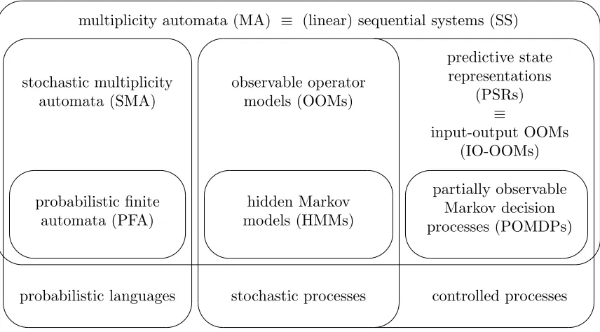
3. Versions of Sequential Systems
stochastic multiplicity automata (SMA)
predictive state representations
(PSRs)
≡
input-output OOMs (IO-OOMs) observable operator
models (OOMs)
probabilistic finite automata (PFA)
hidden Markov models (HMMs)
partially observable Markov decision processes (POMDPs)
stochastic processes controlled processes probabilistic languages
multiplicity automata (MA) ≡ (linear) sequential systems (SS)
Figure 1: SMA, OOMs and PSRs are versions of SSs that model probabilistic languages, stochastic processes and controlled processes respectively, and strictly generalize PFA, HMMs and POMDPs respectively.
3.1 Multiplicity Automata and Weighted Automata
The above definition of linear finite dimensional SS is an equivalent algebraic way of looking at a type of automata that were introduced by Sch¨utzenberger (1961) and are most com-monly known asmultiplicity automata(Salomaa and Soittola, 1978; Berstel and Reutenauer, 1988). We will give a very brief introduction.
Definition 17 A K-multiplicity automaton (MA) is a structure hΣ, Q, ϕ, ι, τi, where Σ is an alphabet, Q is a finite set of states, ϕ : Q×Σ×Q → K is the state transition function, ι : Q → K is the initialization function, and τ : Q → K is the termination function. The state transition function is extended to words by setting ∀x ∈ Σ∗, z ∈ Σ : ϕ(q, xz, q0) = P
s∈Qϕ(q, x, s)ϕ(s, z, q
0), and ϕ(q, ε, q0) = 1 if q = q0 and 0 otherwise. A
multiplicity automaton Mthen defines a function
fM: Σ∗ →K, fM(x) =
X
q,q0∈Q
ι(q)ϕ(q, x, q0)τ(q0).
The formal equivalence of MA to linear finite-dimensional SS is easily seen by rewriting the definition of MA in terms of matrix multiplication: Setωε= [ι(qi)]i, τz = [ϕ(qj, z, qi)]i,j,
and σ= [τ(qj)]>j . Then we haveτxz = [ϕ(qj, xz, qi)]i,j = [Pqk∈Qϕ(qj, x, qk)ϕ(qk, z, qi)]i,j =
[ϕ(qk, z, qi)]i,k[ϕ(qj, x, qk)]k,j = τzτx and similarly fM(x) = στxωε. However, the above
automata (NFA) to WFA that add weights to the initial and terminal states as well as the state transitions. The weight of a path from an initial state to a termination state is then given by the product of the corresponding weights (hence the namemultiplicity automata), while the valuefM(x) is computed by summing the weights of all paths compatible withx.
At this point we should mention that MA as defined here are merely a special case of WFA. The difference is that for MA we consider weights from a field K (here K = R or
K =C), while for WFA the weights are only required to come from an algebraic structureK called a semiring. There exists a large body of theory for WFA that generalizes the theory of SS that we have presented in Section 2, which can be found in the recent textbook by Droste et al. (2009). Note that while MA and WFA are formally closely related, there is a difference in the way they are viewed and used. For instance, WFA are often considered over the semiringR+ with weights given the interpretation of transition probabilities, which are then called probabilistic finite automata (PFA). Such PFA are graphical models, and the states Qare latent states. ForR-MA, however, the weights are allowed to be negative, and the weights as well as the states Q become abstract notions. In other words, PFA (and WFA in general) are typically used when the states and transition structure carry some meaning, while MA are typically used as an abstract tool to characterize functions f : Σ∗→K. This difference in perspective is reflected in the relationship of PFA to SMA, HMM to OOM and POMDP to PSR described in the remainder of this Section 3. Note that PFA are a special case of MA, asR+⊂R. In fact, there exist functionsf : Σ∗→ R+ that can be described by a MA, but not by a PFA, i.e., MA are strictly more general than PFA. This sequence of increasing generalization starting with finite automata (FA) can be summarized as follows:
FA ⊂ NFA ⊂ PFA ⊂ MA≡SS ⊂ WFA.
Furthermore, there exists a natural extension of WFA to input-output systems that are called weighted finite-state transducers (WFST). Here, the alphabet Σ is split as Σ = ΣI×ΣO, where ΣI is regarded as input alphabet and ΣO as output alphabet. The function
fM : Σ∗I×Σ∗O → K is then viewed as describing a relation between ΣI and ΣO. Again,
K is in general only required to be a semiring, but a typical choice is K = R+ with the interpretation of state transition probabilities, yielding a latent variable model called probabilistic finite-state transducers (PFST). WFST are a flexible class of models that have been shown to unify several common approaches used in the the context of language and speech processing; a survey is given by Mohri et al. (2002). Furthermore, IO-OOMs and thereby PSRs (cf. Section 3.2 and Section 3.3) are in fact WFST with weights in K = R, although they are not usually viewed this way, as WFST are typically seen as latent variable models, while IO-OOMs and PSRs are not. However, since PFST are MA, as long as the desired application merely requires the characterization of the functionfM: Σ∗I×Σ∗O→R+, the SS learning algorithms described in Section 4 can be applied to the case of WFST as well, as has been done recently by Balle et al. (2011).
Note that in the context of MA one is usually interested in characterizing functions f : Σ∗ → K, which are also called formal series in general and recognizable series if they
for some threshold parameterκ ≥0. The class of languages recognizable by MA is known to be strictly more general than the class of regular languages (Cortes and Mohri, 2000).
MA have received a lot of attention in the context of learning theory following the discovery of efficient learning algorithms (Bergadano and Varricchio, 1994; Ohnishi et al., 1994) in an extended version of the exact learning model of Angluin (1987). This led to further results on the learnability of several classes of DNF formulae (Bergadano et al., 1996), the class of polynomials over finite fields, decision trees and others (Beimel et al., 1996, 2000).
3.1.1 Stochastic Multiplicity Automata and Stochastic Languages
Additionally, MA have been applied in the context of probabilistic grammatical infer-ence (Denis et al., 2006; Bailly et al., 2009), which is of particular interest to us because of the close relationship of these approaches to OOMs and PSRs — as we shall see.
Definition 18 A function f : Σ∗ →Rthat satisfies 0≤f ≤1 and f(Σ∗) =Px∈Σ∗f(x) = 1is called a stochastic language,probabilistic languageor just distributionover Σ∗. A
dis-tributionfM onΣ∗ that is defined by some MAMis called a rational stochastic language,
and a MA that defines such a distribution is called a stochastic MA (SMA).
Denis and Esposito (2008) give a comprehensive overview of rational stochastic languages over various fields K, their relationships and relations to subclasses such as the important class of probabilistic regular languages.
Definition 19 A probabilistic (finite) automaton (PFA) is a SMA with the following re-strictions: (i)ι, τ, ϕhave values in[0,1], and (ii) ι(Q) = 1and∀q ∈Q:τ(q) +ϕ(q,Σ, Q) = 1, where ι(Q) = P
q∈Qι(q) and ϕ(q,Σ, Q) =
P
x∈Σ P
q0∈Qϕ(q, x, q0). The stochastic lan-guages that can be represented by PFA are called probabilistic regular languages.
PFA are closely related to hidden Markov models (HMMs), and the relationship has been detailed out by Dupont et al. (2005). It is however less well known that SMA are closely related to observable operator models — a class of models for stochastic processes that generalize HMM in a similar way that SMA generalize PFA.
We point out two results that are relevant in the context of modeling probabilistic lan-guages by MA. First of all, it is known that it is an NP-hard problem to compute the maximum likelihood estimate of parameters of a PFA with known structure from a given training set of words (Abe and Warmuth, 1992). In practice, algorithms based on expec-tation maximization (EM) (Dempster et al., 1977) are used which compute locally optimal models instead. In contrast to this, the algebraic theory for SSs allows for powerful learning algorithms (see Section 4) that often outperform EM-trained PFA or HMMs (Rosencrantz et al., 2004; Jaeger et al., 2006a). However, these learning algorithms may return MA that are arbitrarily close to SMA but fail to represent stochastic languages. It is in fact undecidable whether a MA represents a stochastic language (Denis and Esposito, 2004).
3.2 Observable Operator Models and Stochastic Processes
models are closely related to other algebraic characterizations of stochastic processes (Heller, 1965; Ito, 1992; Upper, 1997) that were studied in the context of deciding the equivalence for HMMs (Gilbert, 1959), which came to a successful conclusion by framing HMMs in the more general class oflinearly dependent processes by Ito et al. (1992).
Definition 20 A (discrete-valued) stochastic process is a function f : Σ∗ → [0,1] that
satisfies (i)f(ε) = 1 and (ii) ∀x∈Σ∗ : f(x) =P
x∈Σf(xx). Such a functionf defines the probabilities of initial observation sequences. An observable operator model (OOM) is a linear SS Msuch thatfM is a stochastic process. A stochastic process that can be modeled
by a finite dimensional OOM is called a linearly dependent process.
One of the interesting features of OOMs is their notion of “state” of a (stochastic) process. The idea that goes back to Zadeh (1969) is that a system state is really nothing more than the information that is required to predict the future. In the case of OOMs, the states ωx not only carry enough information to predict the future, they are (in a certain
sense) just future predictions.
To see this, recall that the states ωx of a SS are coordinate representations of the
functions fx w.r.t. some unknown basis B of the function space F. In the case of OOMs,
these functions take on the meaning that fx(y) = P(xy), i.e., they give the probability of
observing the sequencexfollowed byy. These functions are therefore calledfuture prediction functions in the context of OOMs. The operators {τz} are then state update operators
that update a state ωx (corresponding to the future prediction function fx after an initial
observation of x) according to the new observation z to the new stateωxz (corresponding
to the future prediction function fxz after an initial observation of xz) — hence the name
“observable operators” (Jaeger, 1998).
For convenience, these functions fx, as well as the corresponding states ωx, are often
normalized to fx/f(x) and ωx/σωx respectively, since fx(y)/f(x) = στyωx/σωx =P(y|x),
the probability of observingy given thatx has been observed. Therefore, an OOM started in the normalized state ωx/σωx represents a stochastic process started after an initial
ob-servation of x. This corresponds to the notion of a residual automaton in the context of SMA, which is obtained by starting a SMA in the (normalized) stateωx/
P
z∈Σ∗στzωx and then represents aresidual language (Denis and Esposito, 2004).
3.2.1 Relation to Hidden Markov Models
Any HMM can be trivially converted into an OOM. A hidden Markov model (HMM) consists of an unobserved Markov process Xt that takes values in a finite set of states
Q ={s1, . . . , sn}, and is governed by a stochastic state transition matrix T = [P(Xt+1 =
sj|Xt=si)]i,j. At each time step an observationYt from Σ is made according to the
emis-sion vectorEz = [P(Yt=z|Xt=si)]i. Finally, an initial state vector π = [P(X0 =si)]i is
needed to fully specify the distribution of the stochastic process Yt (Rabiner, 1989).
Proposition 21 (Jaeger, 2000b) A given HMM(T,{Ez}z∈Σ, π)withN states is equivalent to the OOM (σ,{τz}, ωε) defined by σ= (1, . . . ,1), τz =T>diag(Ez) and ωε=π. The rank
Moreover, there are examples of OOMs of finite rank that cannot be modeled by any HMM with a finite number of states. A prototypical example is the so-called “probability clock” (Jaeger, 1998). It is an open question how to find a “close” HMM for a given OOM. While OOMs can be seen as a generalization of HMMs, one should keep in mind that there is a fundamental difference in the notion of the state of the process. The state vector in the case of a HMM is a stochastic vector that expresses the belief about the underlying hidden state, while for an OOM it is a coordinate representation of the corresponding future prediction function. However, under certain conditions it is possible to recover HMM-like hidden states from an OOM (Hsu et al., 2009; Anandkumar et al., 2012).
3.2.2 Relationship to Stochastic Multiplicity Automata
The main difference between OOMs and SMA is that OOMs model stochastic processes, while SMA model distributions on words. However, we can use a stochastic process to model a distribution on words if we introduce a termination symbol $.
Definition 22 An OOM Mover the alphabet Σ$ = Σ∪ {$} is terminating iffM(Σ∗$) :=
P
x∈Σ∗στ$τxωε = 1.
Proposition 23 An OOM M = (σ,{τz}, ωε) over the alphabet Σ can be extended to a
terminating OOMM0= (σ,{τ0
z}, ωε)over the alphabetΣ$ = Σ∪{$}by settingτz0 = (1−p)τz
and τ$0 =pτΣ for some fixed termination probability p∈(0,1), where τΣ= P
z∈Στz. Proof We first show that M0 describes a stochastic process. Clearly, f
M0 ≥ 0 and
fM0(ε) = σωε = 1. To show property (ii), take any x ∈ Σ∗
$ and note that by linearity
τx0ωε = Pkλkτxkωε for suitable λk ∈ R and sequences xk ∈ Σ
∗ (this is obtained by
re-placing all occurrences of τ$0 by pP
z∈Στz). Then Pz∈Σ$fM
0(xz) = σ(P
z∈Σ$τ
0
z)τx0ωε =
στΣτx0ωε =PkλkστΣτxkωε =Pkλkστxkωε = στx0ωε =fM0(x). Furthermore, fM0(Σ∗$) = P
x∈Σ∗στ$0τx0ωε =P∞l=0 P
x∈ΣlσpτΣ(1−p)lτxωε=P∞l=0p(1−p)l= 1.
Definition 24 A terminating OOM M over the alphabet Σ∪ {$} and a SMA A over the alphabet Σ are related, if fM(x$) =fA(x) for allx∈Σ∗.
Lemma 25 If A = (σ,{τz}, ωε) is a minimal d-dimensional SMA, then τΣ∗ = P∞
k=0τΣk exists and is equal to (Id−τΣ)−1, where τΣ=Pz∈Στz.
Proof We will show that the spectral radius1 ρ(τ
Σ) satisfies ρ(τΣ) < 1, which implies the lemma. Assume ρ(τΣ) ≥ 1, i.e., there exists some λ ∈ C,|λ| ≥ 1 and v ∈ Cd such that τΣv = λv. As A is minimal, we may find sequences xj, xi ∈ Σ∗ such that
Π = ((στxi)>)>i∈I and Φ = (τxjωε)j∈J with |I| = |J| = d are non-singular using
Algo-rithm 1. Then v = Φa for some a ∈ Cd, and ΠτΣkΦa = λkΠΦa for any k ∈ N. Now the SMA property fA(Σ∗) = P∞k=0στΣkωε = 1 implies that ΠτΣkΦ → 0 as k → ∞, while the right hand sideλkΠΦadoes not (note ΠΦa6= 0), which is a contradiction.
Proposition 26 Let A = (σ,{τz}, ωε) be a minimal d-dimensional SMA. Then M =
(σ0,{τz0}, ω0ε) is a related (d+ 1)-dimensional terminating OOM over the alphabet Σ$ = Σ∪ {$}, if
• σ0 = [σP∞
k=0τΣk,1] = [σ(Id−τΣ)−1,1], • τz0 =τz 0
0 0
, τ$0 = [0 0
σ 1], and • ωε0 = [ωε0 ].
Proof We can simply check that for all z∈Σ∗$
fM(z) =σ0τz0ω
0
ε=
σ(P∞
k=0τΣk)τzωε ifz∈Σ∗,
στxωε ifz=x$. . .$ for some x∈Σ∗,
0 otherwise.
This implies fM ≥ 0, fM(x$) = fA(x) for all x ∈ Σ∗ (M and A are related), as well as fM(Σ∗$) =fA(Σ∗) = 1 (Mis terminating if it is an OOM). Furthermore,σ0ω0ε=fA(Σ∗) =
1 andσ0τΣ0
$ = [σ
P∞
k=0τΣkτΣ+σ,1] =σ0, which imply property (i) and (ii) for a stochastic process respectively.
Proposition 27 Conversely, let M= (σ,{τz}, ωε) be a d-dimensional terminating OOM
over the alphabet Σ∪ {$}. Then A = (στ$,{τz}, ωε) is a related d-dimensional SMA over
the alphabet Σ.
Proof Clearly,fA(x) =fM(x$)≥0 for all x∈Σ∗ and fA(Σ∗) =fM(Σ∗$) = 1.
3.2.3 Historical Remarks
Note that our definition of OOMs given in Definition 20 differs slightly from the definition typically found in the literature.
First of all, the property (ii) for a stochastic process means that an OOM must satisfy στΣωx =σωx for allx ∈Σ∗, which implies (ii)’ στ =σ if the OOM is minimal, but not in
general. The property (ii)’ is however often stated as part of the definition for OOMs. Our above Definition 20 is therefore slightly more relaxed than the standard definition in the case of non-minimal models, but this has no practical consequences.
Furthermore, for purely historical reasons, OOMs are sometimes required to satisfy σ = (1, . . . ,1), which is mainly an issue of normalization (cf. Proposition 13). However, this in turn has led to a more restrictive definition of interpretability for OOMs, since due to property (i) of stochastic processes, an OOM that satisfies σ = (1, . . . ,1) can only be interpretable with respect to sets Yk, if 1 =σωε= (1, . . . ,1)·[fM(Yi)]>i =
P
k
P
y∈YkP(y).
This is typically assured by requiring the sets Yk to partition Σl for somel. One can relax
this restriction on the sets Yk for the definition of interpretability — as we have done in
Nevertheless, even though the normalization requirement σ = (1, . . . ,1) is superfluous, several of the OOM learning algorithms have been designed to yield OOMs normalized such that σ = (1, . . . ,1) — oftentimes unnecessarily complicating the algorithms — and some proofs have made use of this normalization as well. Later in Section 4 we present simplified and generalized versions of the EC and ES learning algorithms by removing this normalization restriction from the algorithms and proofs.
3.3 Predictive State Representations and Controlled Processes
Following the development of OOMs for stochastic processes, extensions to the case of controlled processes — stochastic processes that depend on an external input at each time step — were proposed by Jaeger (1998) asinput-output OOMs, by Littman et al. (2001) as predictive state representationsand as a further variant astransformed PSRsby Rosencrantz et al. (2004). All approaches are (in the linear case) equivalent and can be easily understood in the framework of linear SSs.
Definition 28 A (discrete-valued) controlled (stochastic) process with input from ΣI and
output inΣOis a functionp: Σ∗→[0,1]that satisfies (i)p(ε) = 1and (ii)∀x∈Σ∗, a∈ΣI:
p(x) =P
o∈ΣOp(xao), whereΣ = (ΣI×ΣO)andao= (a, o). We definep(y|x) =p(xy)/p(x)
forp(x)6= 0and zero otherwise. An input-output OOM(IO-OOM) is just a SS that models a controlled process.
Note that the values of p are not probabilities. One may interpret p(a1o1. . . anon) as
P(o1. . . on|a1. . . an), i.e., as the conditional probability of observing the outputs o1. . . on
given the inputs a1. . . an. However, one must take care, as the sequence of inputs may
depend on the observed outputs as well. This is explained in more detail in Section 4.1.
Definition 29 Let p be a controlled process with predictive states ˙ωh defined as ω˙h = [p(q1|h), . . . , p(qd|h)]> ∈Rd for h ∈Σ∗ and some fixed set of sequences qi ∈Σ∗. If ω˙h is a
sufficient statistic for any history h ∈ Σ∗, i.e., for every x ∈ Σ∗ there is a function mx :
Rd → [0,1] such that p(x|h) =mx( ˙ωh) for all h ∈ Σ∗, then the sequences {q1, . . . , qd} are
called core tests, which together with the initial state ˙ωε and projection functionsmx form
a d-dimensional predictive state representation(PSR) forp. If the projection functions are linear functionals (i.e., just row vectors in Rd), then the PSR is called linear.
Note that PSRs share the notion of “state” with OOMs in that the state consists of the information required to predict the future, but PSRs additionally require the entries of the state vectors ˙ωh to be “predictions” p(qi|h) for the core tests qi. Such states are therefore calledpredictive states.
Proposition 30 Let ad-dimensional linear PSR consisting of core testsqi, projection func-tions mx and an initial stateω˙ε for a controlled process p be given. Then an equivalent SS
M= (σ,{τz}, ωε) is obtained by setting
ωε= ˙ωε, τz = [(mzq1)
>, . . . ,(m
zqd)
>]> and σ = X
o∈ΣO
mao for anya∈ΣI.
Furthermore, Mwill be interpretable w.r.t. the sets{qi}.
Proof First note thatσω˙x =Po∈ΣOmaoω˙x =
P
o∈ΣOp(ao|x) = 1 for allx∈Σ
∗ such that
p(x) 6= 0 becausep is a controlled process. Next, we prove that (*)ωx =p(x) ˙ωx and (**)
fM(x) =p(x) by induction on the lengthl ofx:
• Forl= 0 we have ωε=p(ε) ˙ωε and fM(ε) =σωε=σω˙ε= 1 =p(ε).
• Assume (*) and (**) are true for all x ∈ Σl. Let xz ∈ Σl+1. Then (*) ω
xz =
τzωx = τzω˙xp(x) = [p(zqi|x)]>i p(x) = [p(qi|xz)]>i p(z|x)p(x) = ˙ωxzp(xz) and (**)
fM(xz) =σωxz =σω˙xzp(xz) =p(xz).
Note that property (*) says thatωx=p(x) ˙ωx= [p(xq1), . . . , p(xqd)]>for allx, i.e., thatM
is interpretable w.r.t. the sets{qi}.
Proposition 31 Conversely, letM= (σ,{τz}, ωε) be a SS for a controlled processp. Then
an equivalent PSR is obtained by making the SS interpretable with respect to singleton sets {yi} for appropriate sequencesyi∈Σ∗ (e.g., using Algorithm 3). We can then use these as core tests for the PSR, and set mx =στx for allx∈Σ∗.
Proof We assume that the SS has been made interpretable w.r.t. the sequencesy1, . . . , yd. Then the normalized states ˙ωh =ωh/σωh have the form ˙ωh= [p(y1|h), . . . , p(yd|h)]>. Fur-thermore, for allh∈Σ∗: mxω˙h=στxω˙h=στxτhωε/στhωε=p(x|h), as desired.
Corollary 32 A linear PSR can be specified by the parameters ({mao},{Mao}, ω>ε) for
ao∈ΣI×ΣO, where Mao=τao> and mao = (στao)>, and defines a controlled process via
p(a1o1· · ·anon) =ωε>Ma1o1· · ·Man−1on−1manon.
This is the usual way of specifying a PSR.
Note that transformed PSRs (TPSRs) are just PSRs that model controlled processes in the form of Corollary 32 without any further requirements (i.e., without the requirement that the states need to be interpretable). These are readily converted to SSs by setting σ= (P
o∈ΣOmao)
>for anya∈Σ
Iand using the equations from the Corollary 32 otherwise.
3.3.1 Relation to Partially Observable Markov Decision Processes
Finally, we note how to convert POMDPs into SSs (which can then be further converted to PSRs by making the SS interpretable, as described above). A POMDP with d states Q={s1, . . . , sd} for a controlled process with input alphabet ΣI and output alphabet ΣO
consists of an initial belief state b∈Rd whosei-th element is the probability of the model starting in statesi, a state transition matrixTa∈Rd×dfor each actiona∈Asuch that the
i, j-th entry of Ta is the probability of transitioning to statesi from statesj if actiona is
taken, and a vector Oao ∈Rd for each action-observation pair ao∈ (ΣI×ΣO) whose i-th
entry is the probability of observingoafter arriving in statesiby taking actiona(Kaelbling
et al., 1998).
Setting Oao0 = diag (Oao) we can summarize the belief-state update procedure for the
POMDP concisely by stating that a POMDP models a controlled stochastic process p via the equation
p(a1o1· · ·anon) = (1, . . . ,1)(O0anonTan)· · ·(O0a1o1Ta1)b.
Clearly, setting σ = (1, . . . ,1),τao=Oao0 Ta andωε=b yields an equivalent SS.
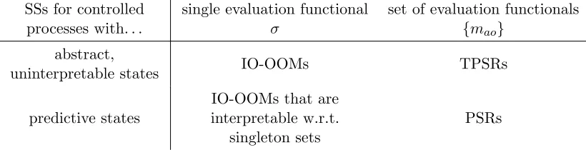
3.3.2 IO-OOMs, Interpretable IO-OOMs, PSRs and TPSRs
We have shown above that IO-OOMs, PSRs and TPSRs are equivalent models in the sense that they model the same class of controlled processes and that they can be readily converted into one another. Furthermore, TPSRs are essentially IO-OOMs (except that the evaluation functionalσ is replaced by the set{mao}of evaluation functionals), while PSRs are TPSRs
(and therefore essentially IO-OOMs) with predictive states, which corresponds to IO-OOMs being interpretable w.r.t. singleton sets (core tests). This is summarized in Table 1.
SSs for controlled processes with. . .
single evaluation functional σ
set of evaluation functionals
{mao}
abstract,
uninterpretable states IO-OOMs TPSRs
predictive states
IO-OOMs that are interpretable w.r.t.
singleton sets
PSRs
Table 1: The differences between IO-OOMs, PSRs and TPSRs
As the original notion of interpretability for IO-OOMs has turned out to be overly restrictive, we propose to employ the notion of interpretability that we have introduced here for SSs as the “correct” notion for IO-OOMs, and consider the original notion as deprecated.
3.3.3 Historical Remarks
The same remarks that we have made above in Section 3.2.3 for OOMs also apply to IO-OOMs. Namely, IO-OOMs were originally required to satisfy (ii)’: ∀a∈ΣI:σPo∈ΣOτao=
σ instead of the the property (ii) for a controlled process. This is equivalent for minimal models, but slightly more restrictive in general. However, as every SS can be minimized, this has no practical consequences.
Furthermore, IO-OOMs were originally typically required to satisfyσ= (1, . . . ,1), which is again merely a matter of normalization. However, an IO-OOM that satisfiesσ= (1, . . . ,1) can only be interpretable with respect to the sets Yk, if 1 =σωε = (1, . . . ,1)·[fM(Yi)]>i =
P
k
P
y∈Ykp(y). It turns out that this can be assured by requiring the setsYk to partition
Σl
O× {a1} × · · · × {al}for someland a fixed sequencea1. . . al of inputs called a
characteri-zation frame. This restriction on the choice of setsYktherefore became part of the original
definition of interpretability for IO-OOMs.
Unfortunately, unlike the case for OOMs, the resulting original notion of interpretability for IO-OOMs has turned out to be a severe limitation (Singh et al., 2004).
However, one may use the more general notion of interpretability given in Definition 14 for IO-OOMs instead, if one is willing to drop the (unnecessary) normalization requirement σ= (1, . . .1).
3.4 Extensions
In this section we have presented SMAs, OOMs and PSRs as versions of linear sequen-tial systems — or more generally weighted finite automata — that model probabilistic languages, stochastic processes and controlled processes respectively, as is summarized in Figure 1. For completeness, we wish to briefly mention some extensions of these basic model types that have been studied, but which are beyond the scope of this paper.
First of all, various non-linear SSs exists. For instance, several versions of quantum finite automata have been studied (Kondacs and Watrous, 1997; Moore and Crutchfield, 2000). One form are SSs (σ,{τx}, ωε ∈ CPd) where the operators τx are unitary and
σ(τxωε) = ||πτxωε||2 for some projection π and the Fubini-Study metric || · || (Moore and
Crutchfield, 2000). A similar type of OOMs exist which are callednorm-OOMs. These are SSs (σ,{τx}, ωε∈Rd) such thatPx∈Στx>τx=I andσ(τxωε) =||τxωε||2. Such norm-OOMs
describe stochastic processes and can always be converted into an equivalent OOM (Zhao and Jaeger, 2010). Recently, quadratic weighted automata have been proposed by Bailly (2011), where a SS M is learnt for √f and a product SS M ⊗ M is constructed that satisfies fM⊗M = fM2 ≈ f. All of these approaches avoid the “negative probabilities
problem”, where the estimated modelfM may violate the requirementfM ≥0. Non-linear
Furthermore, OOMs and PSRs are models for discrete-valued stochastic (controlled) processes. Many real-world processes of interest are, however, continuous-valued. A con-tinuous version of OOMs exists that extends semi-concon-tinuous HMMs (Jaeger, 2000a), and WFST have been similarly extended to allow for continuous inputs (Recasens and Quattoni, 2013). Multivariate continuous inputs and outputs are handled using features of observa-tions by reduced-rank HMMs (Siddiqi et al., 2010). So called predictive linear Gaussian models (PLGs), which are based on PSRs, closely resemble linear dynamical system mod-els (Rudary et al., 2005; Wingate and Singh, 2006a,b; Rudary and Singh, 2006, 2008) and are further generalized by exponential family PSRs (Wingate and Singh, 2008b,a). A gen-eralization of OOMs using Hilbert space embeddings was introduced by Song et al. (2010). This has been further refined and extended to include features and can now be employed — among other things — for controlled processes and to planning in reinforcement learning tasks (Boots and Gordon, 2010; Boots et al., 2010, 2013).
4. Learning
In this section we present a general approach to learning SSs from data. We show how several of the learning algorithms that have been proposed for SMA, OOMs and PSRs can be understood in this framework, and that in fact many of the proposed learning algorithms are closely related.
We begin by establishing a result that lies at the heart of the learning algorithms, which was formulated by Kretzschmar (2001) for the case of OOMs. Assuming a functionfMcan
be described by some minimal SS M, it allows us to reconstruct an equivalent SSM0 from
data given in the form of finitely many function values offM — as long as these are given
exactly and we know the rank dof the underlying modelM. We will therefore refer to the Equations (2) as the learning equations.
Proposition 33 For a minimal d-dimensional SS M = (σ,{τz}, ωε), let {τxjωε|j ∈ J}
and {(στxi>)>|i ∈ I} be finite sets that span the state space W and the co-state space W˜
respectively. Define FI,J = [fM(xjxi)](i,j)∈I×J and FzI,J = [fM(xjzxi)](i,j)∈I×J.
Further-more, define FI,0 = [fM(xi)]i∈I and F0,J = [fM(xj)]>j∈J. Let C ∈Rd×|I| and Q∈ R|J|×d
be rank dmatrices such that CFI,JQ is invertible. Then the SS M0 = (σ0,{τz0}, ωε0) defined as follows is equivalent to M:
σ0 =F0,JQ(CFI,JQ)−1, τz0 =CFzI,JQ(CFI,JQ)−1, ω0ε=CFI,0.
(2)
Furthermore, CFI,J = (ωxj0 )j∈J and CFzI,J = (ω0xjz)j∈J, where ωx0 =τx0ω0ε are states of the
SS M0.
Proof Let Π = ((στxi)>)>i∈I, Φ = (τxjωε)j∈J. ThenFI,J = ΠΦ,FzI,J = ΠτzΦ, FI,0 = Πωε
and F0,J =σΦ. We can then simply calculate τz0 =CΠτzΦQ(CΠΦQ)−1 =CΠτz(CΠ)−1,
as well as ωε0 =CΠωε and σ0 =σΦQ(CΠΦQ)−1 =σ(CΠ)−1. That is, we have shown that
ρΦ = (ρτxjωε)j∈J = (τxj0 ωε0)j∈J, and analogously for CFzI,J.
The matrices C and Q that appear in the learning Equations (2) are indeed arbitrary (provided thatCFI,JQhas the correct dimension dand full rank), as long as the function values fM(x) are given exactly. However, if one only has access to estimates ˆf(x), then
the selection ofC and Qplays a crucial role in obtaining good model estimates, as will be further discussed in Section 4.4.
Furthermore, note that we generally do not know a priori which sets of words to consider such that{τxjωε|j ∈J}and{(στxi>)>|i∈I}span the state and co-state spacesW and ˜W
of M. Proposition 6 guarantees that it suffices to consider all words of length at most d, but the rank dof M is generally unknown as well. Selecting appropriate sets of words xi
and xj and an appropriate model dimensiondare therefore crucial and non-trivial steps in
learning models from data.
We can turn the above Proposition 33 into a generic learning procedure for SSs:
Algorithm 4:General procedure for learning a SS from data
1 Obtain estimates ˆf(x) of the function values f(x) for words x∈Σ∗.
2 Choose finite sets {xj|j∈J},{xi|i∈I} ⊂Σ∗, which we call sets ofindicative and
characteristic words respectively. Then assemble the estimates ˆf(x) into estimates of the matrices ˆFI,J, ˆFzI,J, ˆFI,0 and ˆF0,J.
3 Find a reasonable target dimension dfor the model to be learnt.
4 Choose C ∈Rd×|I| and Q∈R|J|×dcalled the characterizer and indicator, such that CFˆI,JQis invertible.
5 Apply the learning Equations (2) to obtain a model estimate ˆM.
At this point we should clarify what is meant here by learning a model from data. For general MA the goal is often to reconstruct an automaton from as fewmembership queries — obtaining the value f(x) for some x ∈ Σ∗ — and equivalence queries — proposing a
functionh and receiving acounterexample xsuch thath(x)6=f(x) if h6=f — as possible. This is an extended version of the exact learning model of Angluin (1987). However, in the case of SMA, OOMs and PSRs, the external function represents a distribution. Therefore, in these cases it is usual to assume that we observe samples from this distribution and wish to estimate model parameters from the given samples such that the estimated model best describes the underlying distribution — “best” in a sense that depends on the context and the approach taken by a specific learning algorithm.
We should also mention one common problem when learning SMAs, OOMs and PSRs from data. Namely, even if the function fM in question can be described by a SMA, OOM
given SS ˆMsatisfiesfMˆ ≥0, and therefore, whether it is a SMA — a result that carries over to OOMs and PSRs as well (Wiewiora, 2008). In practice, there are three basic ways to deal with this “negative probabilities problem”: First of all, one can resort to alternative models as described in Section 3.4 that preclude the problem by design. For the particular case of quadratic weighted automata the learning procedure presented here still applies (Bailly, 2011), but in general one will need alternative learning algorithms. Secondly, one may attempt to learn a restricted class of SS such as PFA, HMMs or POMDPs by enforcing additional constraints on the parameters of the SS. This can be achieved either by adding a set of convex constraints to a generalized version of the spectral learning method presented in Section 4.4.2 (Balle et al., 2012), or by an additional conversion step (Anandkumar et al., 2012), which however may fail. Finally, one may work with such an “invalid” SS model by employing a simple and effective heuristic as described by Jaeger et al. (2006b, Appendix J) to normalize all model predictions to fall into the desired range.
Finally, we will briefly remark on the runtime characteristics of the above learning procedure. Steps 1 and 2 can be accomplished in time O(N), where N is the size of the training data, for most strategies mentioned in Section 4.2 by employing a suffix tree or similar representation of the training data. For a given target dimension d, Step 4, when solved via the EC (Section 4.4.3) or spectral algorithms (Section 4.4.3), requires the
O(d|I||J|) computation of ad-truncated singular value decomposition (SVD) of ˆFI,J, while the ES algorithm (Section 4.4.4) requires O(d2lmax{|I|,|J|}) operations to compute C, where l is the (generally very small) average length of characteristic and indicative words, andO(d|I||J|) operations to compute Q— per iteration (but one typically uses a constant number of iterations), which therefore amounts to a run-time ofO(d|I||J|) as well. Solving the learning Equations (2) for Step 5 essentially requires the computation of the operators ˆ
τz, which costs O(d|I||J||Σ|) operations. So for a known target dimension d, the above
learning procedure typically requires O(N +d|I||J||Σ|) operations. Step 3 can be solved by computing a dmax-truncated SVD of ˆFI,J for some upper bound dmax < min{|I|,|J|} on the target dimension, which incurs a runtime costs of O(dmax|I||J|), or by using cross-validation, which requires repeatedly performing, for various choices of d, Steps 4 and 5 as well as evaluations on test data of size T, which we assume to be constant, incurring a runtime cost of O(dlog(d)|I||J||Σ|), where dis the finally selected model dimension.
In the following, we will discuss the steps of the learning procedure in more detail.
4.1 Obtaining Estimates fˆ(x)
This step clearly depends on the context we are dealing with. Recall that in the context of SMA, the functions we are considering are distributions on words, while in the context of OOMs and PSRs they represent stochastic processes and controlled processes respec-tively. The following Remarks 34 to 36 summarize how to obtain these estimates in the different scenarios of probabilistic languages, stochastic processes and controlled processes, respectively.
Remark 34 Let f : Σ∗ → [0,1] be a distribution on Σ∗, and let S = (s1, s2, . . . , sN) be
In the case of stochastic processes, one typically observes few (or even just one) long initial realization of the process. In this case it is still possible to obtain the desired estimates if the stochastic process is stationary and ergodic2 by invoking the ergodic theorem and using time-averages as estimates. The same idea is commonly used in the case of controlled processes as well and calledsuffix-history method in the PSR community.
Remark 35 Let f : Σ∗ → [0,1] be a stationary and ergodic stochastic process, and let ¯
s=s1s2. . . sN be a finite initial realization of length N from this process. Then
ˆ
f(x) = #(x) N− |x|+ 1,
where #(x) denotes the number of occurrences of x in the sequence ¯s is a consistent esti-mator forf(x).
In the case of controlled processes the situation is more complicated. It is important to have a good understanding of the meaning of the value f(x) when f is a controlled process andx=a1o1. . . anon∈(ΣI×ΣO)n is some input-output sequence. Intuitively, this
is the probability of the system output o1. . . on conditioned on the system input a1. . . an.
This is sometimes written as f(a1o1. . . anon) = P(o1. . . on|a1. . . an) even though this
notation is misleading, as it suggests that P(o1. . . on|a1. . . an) = PP(a1(a1o1...anonΣ )
O...anΣO), which is
false (Bowling et al., 2006). To clarify this, consider the stochastic process that is specified by the controlled process f together with some system input specification. This stochastic process is governed by probabilities of the form
P(a1o1. . . anon) = n
Y
k=1
P(ok|a1o1. . . ak)· n
Y
k=1
P(ak|a1o1. . . ak−1ok−1).
The second factor in the equation models the system input and is sometimes called the input policy π, while the first factor models the system output and is just the controlled processf. Therefore, forx=a1o1. . . anon,
f(x) =P(o1. . . on|a1. . . an) = n
Y
k=1
P(ok|a1o1. . . ak) =
P(x)
π(x). (3)
Note that for the special case of a blind input policy π — one that does not depend on the observed output, i.e., that satisfiesP(ak|a1o1. . . ak−1ok−1) =P(ak|a1. . . ak−1) for all
x — we in fact do have π(x) =P(a1ΣO. . . anΣO).
From the above Equation (3), the following estimates are derived (Bowling et al., 2006):
Remark 36 Letf : Σ∗ →[0,1]be a controlled process, and lets¯=a1o1. . . aNoN be a finite
initial sample from f according to some input policy π, such that the resulting stochastic process is stationary and ergodic. Then
ˆ f(x) =
n
Y
k=1
#(a1o1. . . akok)
#(a1o1. . . ak)
is a consistent estimator for f(x). If the input policy π is known, then
ˆ
f(x) = #(x) N − |x|+ 1·
1 π(x)
is also a consistent estimator which may be used instead. Again, #(x) denotes the number of occurrences ofx in the sequences¯.
None of the above estimates exploits the rich structure of the matrix F. If required, some of the convex constraints that the matrix F must satisfy can be ensured by applying an additional normalization step to the estimated matrix ˆF, as done by McCracken and Bowling (2006). These convex constraints — including a convex relaxation of the rank constraint — may also be used to infer missing values if some entries ˆf(x) cannot be obtained directly, which becomes relevant in the context of learning more general (e.g., non-stochastic) weighted automata (Balle and Mohri, 2012), or to infer sequence alignment when learning WFST from unaligned input-output sequences (Bailly et al., 2013).
4.2 Choosing Indicative and Characteristic Words
Choosing indicative and characteristic words {xj|j ∈ J},{xi|i ∈ I} ⊂ Σ∗ is equivalent
to selecting which columns J and rows I of the system matrix F to estimate. Clearly, it is only possible to obtain a correct estimate for f if I and J are selected such that rank(F) = d = rank(FI,J). It is however unclear how to satisfy this if the true rank is unknown or even impossible if rank(F) = ∞ — as may often be the case for real-world examples. Determining an appropriate rank for the model will be discussed in the following section.
One approach is, however, to attempt to select minimal sets of indicative and charac-teristic words such that rank(F) = rank(FI,J). Such minimal sets are called sets of core histories and core tests in the context of PSRs, and their selection is called the discovery problem. This problem is easily solved by Algorithm 1 once a (minimal) SS model for f is known. For the case where only function values off are available, an iterative procedure has been proposed (James and Singh, 2004) that, starting with the empty words, adds in each iteration all length-one extensions of previously found core histories and tests, but retains only a minimal set needed to span ˆFI,J. Since any noisy matrix is typically non-singular, some notion of numerical linear independence is used to decide which words to retain in each step. It is important to note that there exist simple examples of finite rank where this iterative procedure fails to deliver sets of core histories and tests (James and Singh, 2004), i.e., it does not in general solve the discovery problem. A similar algorithm called DEES has been proposed in the context of learning SMA (Denis et al., 2006). The algorithms for learning MA in the exact learning framework also work by finding a minimal set of indica-tive and characteristic words, but there it is assumed that the function f may be queried exactly, and furthermore equivalence queries are employed to find additional core tests and histories (Ohnishi et al., 1994; Bergadano and Varricchio, 1994; Beimel et al., 2000).
training data will enter the model estimation, i.e., the available data will be under-exploited. It is therefore desirable to use (much) larger sets of indicative and characteristic words than strictly needed.
An approach which is in some sense complementary is to use all sequences of a given length l. By Proposition 6 one can ensure rank(FI,J) = d by choosing l ≥ d. However, this is highly impractical, since the size of ˆFI,J grows exponentially with l. Also, many of the estimates in ˆFI,J will be based on very few — if any — occurrences in the available training data. Nevertheless, choosing a length l dand utilizing as indicative as well as characteristic words all words of lengthlthat occur at least once in the training data often gives good results (Zhao et al., 2009a).
A further approach is to select as indicative and characteristic words all those that actually occur in the data and therefore allow data-based estimates (Bailly et al., 2009). However, it is reasonable to disallow indicative (resp. characteristic) words that are suffixes (resp. prefixes) of some other indicative (resp. characteristic) word if they always occur at the same positions in the training data, as these would just lead to identical columns (resp. rows) in the estimated matrices that are based on the same parts of the training data (Jaeger et al., 2006b). Moreover, one may select only the words that occur most frequently in the data (Balle et al., 2014). These approaches yield a choice of indicative and characteristic words that is matched to the available training data and can be computed in time O(N) where N is the size of the training data by using a suffix tree or similar representation of the training data.
Finally, it is also possible to group words into sets of words (as is also done in Defini-tion 14) that we callevents, and to use indicative and characteristic events in place of words. This corresponds to adding the respective columns and rows in the matrices ˆFI,J,FˆI,J
z , etc.
and can be formally accomplished by a special selection of the indicator and character-izer matrices Qand C. Finding good indicative and characteristic events was the strategy adopted by early OOM learning algorithms (Jaeger, 2000b). A further generalization of this idea of considering events in place of words is proposed by Wingate et al. (2007). Using such events may carry an additional advantage if the estimation of ˆf(Y) from the available data can be performed more efficiently or accurately than computing ˆf(Y) =P
x∈Y fˆ(x).
4.3 Determining the Model Rank