Optimal Learning Rates for Localized SVMs
Mona Meister [email protected]
Corporate Research Robert Bosch GmbH 70465 Stuttgart, Germany
Ingo Steinwart [email protected]
Institute for Stochastics and Applications University of Stuttgart
70569 Stuttgart, Germany
Editor:Sara van de Geer
Abstract
One of the limiting factors of using support vector machines (SVMs) in large scale ap-plications are their super-linear computational requirements in terms of the number of training samples. To address this issue, several approaches that train SVMs on many small chunks separately have been proposed in the literature. With the exception of random chunks, which is also known as divide-and-conquer kernel ridge regression, however, these approaches have only been empirically investigated. In this work we investigate a spa-tially oriented method to generate the chunks. For the resulting localized SVM that uses Gaussian kernels and the least squares loss we derive an oracle inequality, which in turn is used to deduce learning rates that are essentially minimax optimal under some standard smoothness assumptions on the regression function. In addition, we derive local learning rates that are based on the local smoothness of the regression function. We further intro-duce a data-dependent parameter selection method for our local SVM approach and show that this method achieves the same almost optimal learning rates. Finally, we present a few larger scale experiments for our localized SVM showing that it achieves essentially the same test error as a global SVM for a fraction of the computational requirements. In addition, it turns out that the computational requirements for the local SVMs are similar to those of a vanilla random chunk approach, while the achieved test errors are significantly better.
Keywords: least squares regression, support vector machines, localization
1. Introduction
Based on a training set D := ((x1, y1), . . . ,(xn, yn)) of i.i.d. input/output observations drawn from an unknown distribution P on X×Y, where X ⊂Rd and Y ⊂R, the goal of
non-parametric least squares regression is to find a function fD : X → R that is a good
estimate of the unknown conditional mean f∗(x) := E(Y|x), x ∈ X. For this classical
estimation problem various methods have been proposed and studied in the literature, see e.g., (Simonoff, 1996) and the book (Gy¨orfi et al., 2002) for detailed accounts.
In this paper, we consider kernel-based regularized empirical risk minimizers, also known as support vector machines (SVMs), which solve the regularized problem
fD,λ∈arg min f∈Hλkfk
2
Here, λ > 0 is a fixed real number and H is a reproducing kernel Hilbert space (RKHS) over X with reproducing kernel k : X×X → R, see e.g., (Aronszajn, 1950; Berlinet and
Thomas-Agnan, 2004; Steinwart and Christmann, 2008). The function L: X×Y ×R →
[0,∞) is a loss function, where in the following we either consider the least squares loss
LLS : Y ×R → [0,∞) defined by (y, t) 7→ (y−t)2, or variants of it that may depend on
x∈X. Besides, RL,D(f) denotes the empirical risk of a functionf :X →R, that is
RL,D(f) =
1
n
n X
i=1
L(xi, yi, f(xi)) ,
where D is the empirical measure associated to the data Ddefined by D := n1Pn
i=1δ(xi,yi)
with Dirac measure δ(xi,yi) at (xi, yi). Recall that the empirical SVM solution fD,λ exists
and is unique (cf. Steinwart and Christmann, 2008, Theorem 5.5) whenever the loss L is convex in its last argument, which is true for the least squares loss and its variants that will be considered later on. Moreover, an SVM isL-risk consistent under a few assumptions on the RKHS H and the regularization parameter λ, see (Steinwart and Christmann, 2008, Section 6.4) for more details.
An essential theoretical task, which has attracted many considerations, is the inves-tigation of learning rates for SVMs. For example, such rates for SVMs using the least squares loss and generic kernels can be found in (Cucker and Smale, 2002; De Vito et al., 2005; Smale and Zhou, 2007; Caponnetto and De Vito, 2007; Mendelson and Neeman, 2010; Steinwart et al., 2009) and the references mentioned therein. At this point, we do not want to take a closer look at these results, instead we relegate to (Eberts and Steinwart, 2013), where a detailed discussion can be found. More important for our purposes is the fact that Eberts and Steinwart (2011, 2013) establish (essentially) asymptotically optimal learning rates for least squares SVMs (LS-SVMs) using Gaussian RBF kernels. More precisely, for a domain X ⊂B`d
2, Y := [−M, M] with M >0, a distribution P onX×Y such that PX
has a bounded Lebesgue density onX, and forf∗ contained in the Sobolev spaceW2α(PX),
α∈N, or in the Besov-like spaceB2α,∞(PX), α≥1, respectively, the LS-SVM using
Gaus-sian kernels learns for allξ >0 with raten−2α2α+d+ξ with a high probability. In other words,
it learns at least with a rate that is arbitrarily close to the optimal learning rate.
Although these rates are essentially asymptotically optimal, they depend on the order of smoothness of the regression function on the entire input space X. That is, if the regression function f∗ is on some area of X smoother than on another area, the learning rate is determined by the part of X, where the regression function f∗ is least smooth. In contrast to this, it would be desirable to achieve a learning rate on every region of X that corresponds with the order of smoothness of f∗ on this region. Therefore, one of our goals of this paper is to modify the standard SVM approach such that we achieve local learning rates that are asymptotically optimal.
Here the basic idea of most other local approaches is to a) split the training data and just consider a few examples near a testing sample, b) train on this small subset of the training data, and c) use the solution for a prediction w.r.t. the test sample. Here, many up-to-date investigations use SVMs to train on the local data set but, yet there are different ways to split the whole training data set into smaller, local sets. For example, Chang et al. (2010); Wu et al. (1999); Bennett and Blue (1998) use decision trees while in (Hable, 2013; Segata and Blanzieri, 2010, 2008; Blanzieri and Melgani, 2008; Blanzieri and Bryl, 2007a,b; Zhang et al., 2006) local subsets are built considering k nearest neighbors. The latter approaches further vary, for example, Zhang et al. (2006); Blanzieri and Bryl (2007a); Hable (2013) consider different metrics w.r.t. the input space whereas Segata and Blanzieri (2008); Blanzieri and Melgani (2008); Blanzieri and Bryl (2007b) consider metrics w.r.t. the feature space. Nonetheless, the basic idea of all these articles is that an SVM problem based on k training samples is solved for each test sample. Another approach using k
nearest neighbors is investigated in (Segata and Blanzieri, 2010). Here, k-neighborhoods consisting of training samples and collectively covering the training data set are constructed and an SVM is calculated on each neighborhood. The prediction for a test sample is then made according to the nearest training sample that is a center of ak-neighborhood. As for the other nearest neighbor approaches, however, the results are mainly experimental. An exception to this rule is (Hable, 2013), where universal consistency for localized versions of SVMs, or more precisely, a large class of regularized kernel methods, is proven. Another article presenting theoretical results for localized versions of learning methods is (Zakai and Ritov, 2009). Here, the authors show that a consistent learning method behaves locally, i.e., the prediction is essentially influenced by close by samples. However, this result is based on a localization technique considering only training samples contained in a neighborhood with a fixed radius and center x when an estimate in x is sought. Probably closest to our approach is the one examined in (Cheng et al., 2010) and (Cheng et al., 2007), where the training data is split into clusters and then an SVM is trained on each cluster. However, the presented results are again only of experimental character.
Unlike in the papers mentioned above, our main goal is to theoretically investigate local SVMs based on local splitting. Namely, we establish both global and local learning rates for our local splitting approach (VP-SVM) that do match the best existing and essentially optimal rates for global SVMs derived by Eberts and Steinwart (2013). In addition, we show that these rates can be obtained without knowing characteristics of P by a simple and well-known hold-out technique. Furthermore, we empirically compare our VP-SVM to another data splitting approach known as random chunking (RC-SVM) or divide-and-conquer kernel ridge regression for which learning rates, at least for generic kernels, have been recently established by Zhang et al. (2015); Lin et al. (2016). In these experiments it turns out that for splittings that lead to comparable training times, our VP-SVM has a significantly smaller test error than RC-SVMs.
imply f∗ ∈C∞, which is usually considered to be too restrictive. For a similar reason the results by Rudi et al. (2015) for the popular Nystr¨om method require too restrictive assump-tions when applied to SVMs with Gaussian kernels. On a side note, we like to mention that this difference between generic kernels on the one hand and Gaussian kernels on the other hand already appears for the standard global SVMs. Indeed, in the generic case, one usually addresses the approximation error by assuming the conditional mean to be contained in the image of a fractional integral operator, which can in turn be identified as an interpolation space of the real method, see (Steinwart and Scovel, 2012). For certain kernels, the classical theory of interpolation spaces then identifies the considered interpolation spaces as Besov spaces, so that the approximation error assumption has a clear intuitive meaning. On the other hand, for Gaussian kernels with fixed width it has been shown by Smale and Zhou (2003) that their interpolation spaces consist of C∞-functions, so that the generic theory would again lead to a too restrictive approximation error assumption. To address this issue, one considers widths that change with the sample size. However, to make this approach successful, one requires both a manual estimation of the approximation error, see (Eberts and Steinwart, 2011), and eigenvalue/entropy number bounds that do depend on the kernel width. For these reasons, learning rates for SVMs with Gaussian kernels under realistic assumptions are, in general, harder to obtain. Nonetheless, they are important, since in practice, Gaussian kernels are by far the most often used kernels.
The rest of this paper is organized as follows: In Section 2 we describe our splitting approach in detail. Section 3 then presents some theoretical results on RKHSs that enable the analysis of our method. After that, Section 4 contains the main results, namely an oracle inequality and learning rates for our localized SVM method. Moreover, a data-dependent parameter selection method is studied that induces the same rates. Section 5 then presents some experimental results w.r.t. the localized SVM technique. Finally, Section 6 collects the proofs for the results of the earlier sections as well as some necessary and important ancillary findings.
2. Description of the Localized SVM Approach
In this section, we introduce some general notations and assumptions. Based on the latter we modify the standard SVM approach. Let us start with the probability measure P on
X×Y, whereX ⊂Rdis non-empty,Y := [−M, M] for someM >0, and P
X is the marginal distribution of X. Depending on the learning target one chooses a loss function L, i.e., a function L : X×Y ×R → [0,∞) that is measurable. Then, for a measurable function
f :X →R, theL-risk is defined by
RL,P(f) =
Z
X×Y
L(x, y, f(x))dP(x, y)
and the optimalL-risk, called the Bayes risk with respect to P and L, is given by
R∗L,P:= inf{RL,P(f) |f :X →Rmeasurable} .
A measurable function fL,∗P : X → R with RL,P(fL,∗P) = R∗
L,P is called a Bayes decision
In this case, it seems obvious to consider estimators with values in [−M, M] onX. To this end, we introduce the concept of clipping the decision function. LetÛt be the clipped value
of some t∈Rat±M defined by
Û
t:=
−M ift <−M
t ift∈[−M, M]
M ift > M .
Then, a loss is called clippable at M >0 if, for all (x, y, t)∈X×Y ×R, we have
L(x, y,Ût)≤L(x, y, t).
Obviously, the latter implies RL,P(fÛ) ≤ RL,P(f) for all f : X → R. In other words,
restricting the decision function to the interval [−M, M] containing our labels cannot worsen the risk, in fact, clipping this function typically reduces the risk. Hence, we consider the clipped version fÛD of the decision function as well as the riskRL,P(fÛD) instead of the risk RL,P(fD) of the unclipped decision function. Note that this clipping idea does not change
the required solver since it is performedafter the training phase.
To modify the standard SVM approach (1), we assume that (Aj)j=1,...,m is a partition ofX such that all its cells have non-empty interior, that is ˚Aj 6=∅for every j∈ {1, . . . , m}. Now, the basic idea of our approach is to consider for each cell of the partition an individual SVM. To describe this approach in a mathematically rigorous way, we have to introduce some more definitions and notations. Let us begin with the index set
Ij :=
i∈ {1, . . . , n}:xi ∈Aj , j= 1, . . . , m ,
indicating the samples ofD contained inAj, as well as the corresponding data set
Dj :={(xi, yi)∈D:i∈Ij}, j= 1, . . . , m .
Moreover, for every j∈ {1, . . . , m}, we define a (local) lossLj :X×Y ×R→[0,∞) by
Lj(x, y, t) :=1Aj(x)L(x, y, t),
whereL:X×Y ×R→[0,∞) is the loss that corresponds to our learning problem at hand. We further assume thatHj is an RKHS over Aj with kernelkj :Aj×Aj →R. Here, every
functionf ∈Hj is only defined onAj even though a functionfD :X →Ris finally sought.
To this end, for f ∈Hj, we define the zero-extension ˆf :X →Rby
ˆ
f(x) := (
f(x), x∈Aj, 0, x /∈Aj.
Then, the space ˆHj :={fˆ:f ∈Hj} equipped with the norm
is an RKHS on X (cf. Lemma 2), which is isometrically isomorphic to Hj. With these preparations we can now formulate our local SVM approach. To this end, for every j ∈ {1, . . . , m}, we consider the local SVM optimization problem
fDj,λj = arg min ˆ
f∈Hˆjλj kfˆk2
ˆ
Hj+
1
n
n X
i=1
Lj(xi, yi,fˆ(xi)), (2)
where λj > 0 for everyj ∈ {1, . . . , m}. Based on these empirical SVM solutions, we then define the decision functionfD,λ:X→Rby
fD,λ(x) :=
m X
j=1
fDj,λj(x) =
m X
j=1
1Aj(x)fDj,λj(x), (3)
where λ := (λ1, . . . , λm). Since all fDj,λj in (2) are usual empirical SVM solutions the
common properties hold. Moreover, for arbitrary j ∈ {1, . . . , m},fDj,λj(xi) = 0 if xi ∈/ Aj
for alli∈ {1, . . . , n}. Furthermore, note that the SVM optimization problem (2) equals the SVM optimization problem (1) usingHj,Dj, and the regularization parameter ˜λj := |Inj|λj.
That is, fDj,λj as in (2) and hDj,λ˜j := arg minf∈Hj
˜
λjkfk2Hj +RL,Dj(f) coincide on Aj.
Besides, it is easy to show that, whenever a Bayes decision function fL,∗P w.r.t. P and L
exists, it additionally is a Bayes decision function w.r.t. P andLj.
Let us now briefly discuss the required computing time of our modified SVM. To this end, recall that the costs for solving an usual SVM problem areO(nq) where q∈[2,3]. For the new approach we consider m working sets of size n1, . . . , nm where for simplicity we assume ni ≈ mn for all i∈ {1, . . . , m}. Then for each working set an usual SVM problem has to be solved such that, altogether, the modified SVM induces a computational cost of
O m mnq
. Therefore, if m ≈nβ for some β > 0, then our approach is computationally cheaper than a traditional SVM. Note that our strategy using a partition of the input space is a typical way to speed-up SVMs. Other techniques that possess similar properties are, e.g., applied in the articles cited in the introduction. Besides, we refer to (Tsang et al., 2007) and (Tsang et al., 2005) using enclosing ball problems to solve an SVM, to (Graf et al., 2005) presenting an model of multiple filtering SVMs and to (Collobert et al., 2001) investigating a mixture of SVMs based on several subsets of the training set.
To describe the above SVM approach (Aj)j=1,...,m only has to be some partition of X. However, for the theoretical investigations concerning learning rates of our new approach, we have to further specify the partition. To this end, we denote the closed unit ball of the
d-dimensional Euclidean space`d2 by B`d
2 and we define balls B1, . . . , Bm with radiusr >0
and mutually distinct centersz1, . . . , zm∈B`d 2 by
Bj :=Br(zj) :={x∈Rd:kx−zjk2≤r}, j∈ {1, . . . , m}, (4)
wherek · k2 is the Euclidean norm inRd. Moreover, we chooser and z1, . . . , zm such that
B`d 2 ⊂
m [
j=1
i.e., such that the ballsB1, . . . , Bm coverB`d
2 and, simultaneously, any non-empty set X⊂
B`d
2 (cf. Figure 1). The following well-known lemma relates the radius of such a cover with
the number of centers.
Lemma 1 For all c >0 and r∈ (0, c], there exist balls (Br(zj))j=1,...,m with radius r and centers z1, . . . , zm∈cB`d
2 such that
Sm
j=1Br(zj) covers cB`d
2 and r ≤3cm
−1 d.
For simplicity of notation, we assume in the following that X ⊂ B`d
2. Thus, according to
Lemma 1, there exists a cover (Bj)j=1,...,m of X with
r ≤3m−1d. (5)
Let us finally specify the partition (Aj)j=1,...,m of X by the following assumption.
(A) Letr ∈(0,1] and (A0j)j=1,...,me be a partition ofB`d2 such that ˚A
0
j 6=∅as well as ˚A0j =A0j for everyj∈ {1, . . . ,me}and such that there exist ballsBj :=Br(zj)⊃A0j with radius
r and mutually distinct centers z1, . . . , zme ∈ B`d2 satisfying (5). In addition, assume that X is a non-empty, closed subset of B`d
2 satisfying ˚X =X. W.l.o.g. we assume
that, for some m ≤ me, A0j ∩X˚ 6= ∅ for all j ∈ {1, . . . , m} and A0j ∩X˚ = ∅ for all
j∈ {m+ 1, . . . ,me}. Then we define A00j :=A0j ∩X˚ for allj ∈ {1, . . . , m} and assume that (Aj)j=1,...,m is a partition ofX satisfying A00j ⊂Aj ⊂A00j.
Note that the partition (Aj)j=1,...,m of X in Assumption (A) satisfies, for every j ∈
{1, . . . , m},Aj ⊂Bj forBj as in (A)and ˚Aj 6=∅, where the latter is shown in Lemma 8 in the Appendix. Obviously, for the partition (Aj)j=1,...,m,r andm fulfill (5).
In Assumption (A) (A0j)j=1,...,me is a partition of B`d2 from which we build a partition (Aj)j=1,...,mof X⊂B`d
2. However, for the construction of our local SVM approach and the
proofs of the belonging learning rates, it will be negligible whether we first consider a par-tition (A0j)j=1,...,em ofB`d
2 or only a partition (Aj)j=1,...,m ofX, since the cellsA
0
m+1, . . . A0me, which are removed, have zero mass w.r.t. the marginal distribution PX ofX ifPX(∂X) = 0. In the remaining sections we will frequently refer to Assumption (A). Thus, let us illustrate by the following example that (A)is indeed a natural assumption.
Example 1 For somer∈(0,1], let us consider anr-netz1, . . . , zm ofB`d
2, wherez1, . . . , zm
are mutually distinct. Moreover, we assume that X ⊂B`d
2 satisfies
˚
X =X. Based on the
r-net z1, . . . , zm, a Voronoi partition (Aj)j=1,...,m of X is defined by
Aj :=
x∈X: min arg min k∈{1,...,m}
kx−zkk2=j
, (6)
cf. Figure 2. That is,Aj contains all x∈X such that the center zj is the nearest center to
x, and in the case of ties the center with the smallest index is taken. Obviously, (Aj)j=1,...,m
is a partition ofX withA˚j 6=∅andAj ⊂Br(zj)for allj∈ {1, . . . , m}, and hence it satisfies
r z
j
Bj X
Figure 1: Cover (Bj)j=1,...,m of X, where
B1, . . . , Bmare balls with radiusr and centerszj (j = 1, . . . , m).
X
zj
Aj
Figure 2: Voronoi partition (Aj)j=1,...,mofX defined by (6), whereAj ⊂Bj for every j∈ {1, . . . , m}.
Motivated by Example 1, we call the learning method producing fD,λ given by (3) a
Voronoi partition support vector machine, in short VP-SVM. Despite this name, however,
we just take a partition (Aj)j=1,...,m satisfying (A) as basis here instead of requesting (Aj)j=1,...,m to be a Voronoi partition.
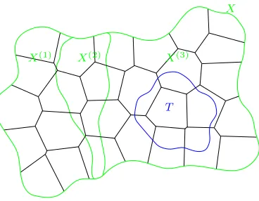
Recall that our goal is to derive not only global but also local learning rates for this VP-SVM approach. To this end, we additionally consider aT ⊂X with PX(T)>0. Then we examine the learning rate of the VP-SVM on this subsetT ofX. To formalize this, it is necessary to introduce some basic notations related toT. Let us define the index set JT by
JT :={j∈ {1, . . . , m}:Aj∩T 6=∅} (7)
specifying every set Aj that has at least one common point with T. Note that, for every non-empty set T ⊂X, the index set JT is also non-empty, i.e., |JT| ≥1. Besides, deriving local rates on T requires us to investigate the excess risk of the VP-SVM with respect to the distribution P and the lossLT :X×Y ×R→[0,∞) defined by
LT(x, y, t) :=1T(x)L(x, y, t). (8)
However, to manage the analysis we additionally need the lossLJT :X×Y ×R→[0,∞)
given by
LJT(x, y, t) :=1Sj∈JTAj(x)L(x, y, t), (9)
which may only be nonzero, if x is contained in some set Aj with j ∈JT. Note that the risks RLT,P(f) and RL
JT,P(f) quantify the quality of some functionf just onT and
AT := [
j∈JT
Aj ⊃T ,
respectively. Hence, examining the excess risks
RLT,P(fÛD,λ)− R∗L
T,P≤ RLJT,P(fÛD,λ)− R
∗
T
X
X(1) X(2) X(3)
Figure 3: The input spaceX with the corresponding partition (Aj)j=1,...,mand the subsetT, where the local learning rate should be examined.
leads to learning rates on AT and implicitly on T. Recapitulatory, let us declare a set of notations that will be frequently used in the remainder of the paper.
(T) For T ⊂X, we define an index set JT by (7), loss functionsLT, LJT :X×Y ×R→
[0,∞) by (8) and (9), and the set AT := S
j∈JTAj.
3. Building Weighted Global Kernels
In this section, we first focus on RKHSs and direct sums of RKHSs. Then, we show that a VP-SVM solution is also the solution of an usual SVM.
Let us begin with some basic notations. For q ∈[1,∞] and a measure ν, we denote by
Lq(ν) the Lebesgue spaces of order q w.r.t. ν and for the Lebesgue measureµ on X ⊂Rd we writeLq(X) := Lq(µ). In addition, for a measurable space X, the set of all real-valued measurable functions on X is given by L0(X) := {f :X → R|f measurable}. Moreover,
for a measure ν on X and measurable Xe ⊂X, we define the trace measure ν| e
X of ν inXe by ν|
e
X(A) =ν(A∩Xe) for everyA⊂X.
Our first goal is to show that fD,λ in (3) is actually an ordinary SVM solution. To
this end, we consider an RKHS on some A (X and extend it to an RKHS on X by the
following lemma, where we omit the obvious proof.
Lemma 2 Let A ⊂ X and HA be an RKHS on A with corresponding kernel kA. Denote
by fˆthe zero-extension of f ∈HA toX defined by
ˆ
f(x) := (
f(x), for x∈A ,
0, for x∈X\A .
Then, the space HˆA:={fˆ:f ∈HA} equipped with the norm kfˆkHˆ
A :=kfkHA is an RKHS
onX and its reproducing kernel is given by
ˆ
kA(x, x0) := (
kA(x, x0), if x, x0∈A ,
Based on this lemma, we are now able to construct an RKHS by a direct sum of RKHSs ˆ
HA and ˆHB with A, B ⊂X and A∩B =∅. Here, we skip the proof once more, since the assertion follows immediately using, for example, orthonormal bases of ˆHA and ˆHB.
Lemma 3 For A, B⊂X such thatA∩B =∅ and A∪B⊂X, let HA andHB be RKHSs
of the kernels kA and kB over A and B, respectively. Furthermore, letHˆA and HˆB be the
RKHSs of all functions of HA and HB extended to X in the sense of Lemma 2 and let kˆA
and ˆkB given by (10) be the associated reproducing kernels. Then, HˆA∩HˆB = {0} and
hence the direct sum
H := ˆHA⊕HˆB (11)
exists. For λA, λB>0 andf ∈H, let fˆA∈HˆA and fˆB ∈HˆB be the unique functions such
thatf = ˆfA+ ˆfB. Then, we define the norm k · kH by
kfk2
H :=λAkfˆAk2Hˆ A+λB
kfˆBk2Hˆ
B (12)
and H equipped with the norm k · kH is again an RKHS for which
k(x, x0) :=λ−A1kˆA(x, x0) +λ−B1kˆB(x, x0), x, x0 ∈X , is the reproducing kernel.
To relate Lemmas 2 and 3 with (3), we have to introduce some more notations. For pairwise disjoint sets A1, . . . , Am⊂X, let Hj be an RKHS onAj for every j∈ {1, . . . , m}. Then, based on RKHSs ˆH1, . . . ,Hˆm on X defined by Lemma 2, a joined RKHS can be designed analogously to Lemma 3. That is, for an arbitrary index set J ⊂ {1, . . . , m} and a vector λ= (λj)j∈J ∈(0,∞)|J|, the direct sum
HJ := M
j∈J ˆ
Hj =
f =X j∈J
fj :fj ∈Hˆj for all j∈J
(13)
is again an RKHS equipped with the norm
kfk2
HJ =
X
j∈J
λjkfjk2Hˆj. (14)
IfJ ={1, . . . , m}, we simply writeH:=HJ. Note thatH contains inter aliafD,λgiven by
(3).
Let us briefly investigate the regularized empirical risk offD,λ=
Pm
j=11AjfDj,λj, where
fDj,λj,j= 1, . . . , m, are defined by (2). For an arbitraryf ∈H, we have
kfD,λk2H +RL,D(fÛD,λ) =
m X
j=1
λj
fDj,λj
2 ˆ
Hj+RLj,D( Û
fD,λ)
≤
m X
j=1
λj
1Ajf
2 ˆ
Hj +RLj,D(f)
=kfk2H +RL,D(f), (15) where we usedRL,D(f) =Pjm=1RLj,D(f), which immediately follows by Lemma 9 given in
the appendix. That is, fD,λ is the decision function of an SVM using H and L as well as
the regularization parameter ˜λ= 1. In other words, the latter SVM equals the VP-SVM given by (3). This will be a key insight used in our analysis.
Subsequently, we only consider RKHSs of Gaussian RBF kernels. For this purpose, we summarize some assumptions for the Gaussian case of joined RKHSs in the following assumption set.
(G) For pairwise disjoint subsets A1, . . . , Am of X, letHj :=Hγj(Aj),j∈ {1, . . . , m}, be
the RKHS of the Gaussian kernel kγj with width γj ∈(0, r] over Aj. Consequently,
forλ:= (λ1, . . . , λm)∈(0,∞)m, we define the joined RKHSH :=Lmj=1Hˆγj(Aj) and
equip it with the norm (14).
In the following we do not consider SVMs with a fixed kernel, thus, we use a more detailed notation than (2) and (3) specifying the kernel widthγj of the RKHS Hγj(Aj) at
hand. Namely, for allj∈ {1, . . . , m} andγ := (γ1, . . . , γm), we write
fDj,λj,γj = arg min
f∈Hˆγj(Aj)
λjkfk2Hˆ
γj(Aj)+
1
n
n X
i=1
Lj(xi, yi, f(xi)),
and
fD,λ,γ :=
m X
j=1
fDj,λj,γj
instead offDj,λj andfD,λin the remainder of this work.
4. Learning Rates for Least Squares VP-SVMs
In this section, the non-parametric least squares regression problem is considered using the least squares loss L:Y ×R→[0,∞) defined byL(y, t) := (y−t)2. It is well known that,
in this case, the Bayes decision function fL,∗P :Rd→ R is given by fL,∗P(x) = EP(Y|x) for
PX-almost all x ∈Rd. Moreover, this function is unique up to zero-sets. Besides, for the
least squares loss the equality
RL,P(f)− R∗L,P=f−fL,∗P
2
L2(PX)
4.1 Basic Oracle Inequalities for LS-VP-SVMs
To formulate oracle inequalities and derive rates for VP-SVMs using the least squares loss, the target functionfL,∗Pis assumed to satisfy certain smoothness conditions. To this end, we initially recall the modulus of smoothness, a device to measure the smoothness of functions, see e.g., DeVore and Lorentz, 1993, p. 44; DeVore and Popov, 1988, p. 398; as well as Berens and DeVore, 1978, p. 360. Denote byk · k2 the Euclidean norm and let Ω⊂Rd be a subset
with non-empty interior, ν be an arbitrary measure on Ω, p ∈ (0,∞], and f : Ω → R be contained inLp(ν). Then, fors∈N, thes-th modulus of smoothness off is defined by
ωs,Lp(ν)(f, t) = sup
khk2≤t
k4sh(f, ·)kLp(ν) , t≥0 ,
where4s
h(f, ·) denotes thes-th difference off given by
4sh(f, x) = (Ps
j=0
s j
(−1)s−jf(x+jh) ifx∈Ωs,h
0 ifx /∈Ωs,h
for h = (h1, . . . , hd) ∈ Rd and Ωs,h := {x∈Ω :x+th∈Ω f.a. t∈[0, s]}. Based on the modulus of smoothness, we introduce Besov-like spaces, i.e., function spaces that provide a finer scale of smoothness than the commonly used Sobolev spaces and that will thus be assumed to contain the target function later on. To this end, let α >0, s:= bαc+ 1, and
ν be an arbitrary measure. Then, the Besov-like spaceB2α,∞(ν) is defined by
Bα2,∞(ν) :=
n
f ∈L2(ν) :|f|Bα
2,∞(ν)<∞ o
,
where the semi-norm | · |Bα
2,∞(ν) is given by
|f|Bα
2,∞(ν):= sup t>0
t−αωs,L2(ν)(f, t)
and the norm by kfkBα
2,∞(ν) := kfkL2(ν) +|f|B2α,∞(ν). Here, note that we defined Besov-like spaces for arbitrary measures ν on Ω⊂Rd whereas in the literature Besov spaces are usually defined for the Lebesgue measure. Nevertheless, our definition of Besov-like spaces is well-defined. Moreover, for the proofs it is important to notice that, if Ω =Rdand ν is a
distribution on Ω with suppν (Ω, then Ωs,h still equals Rd, i.e., Ωs,h= Ω. Also note that for the Lebesgue measure on Ω, where Ω =Rdor Ω is a bounded Lipschitz domain inRd, our
definition of Besov-like spaces actually coincides, up to equivalent norms, to the definition of the classical Besov spaces in the literature, see e.g., (Adams and Fournier, 2003, Section 7), (Triebel, 2006, Section 1), (Triebel, 1992, Section 1), and (Triebel, 2010, Sections 2 and 3), where this classical type of Besov spaces is also defined for 1 ≤ p, q ≤ ∞ and α > 0. For more details on the equivalences of our definition of Besov-like spaces and the classical definitions, we refer to (Eberts, 2015, Section 3.1). If ν is the Lebesgue measure on Ω, we writeB2α,∞(Ω) :=Bα2,∞(ν). Additionally, let us briefly consider a few embedding properties for Besov-like spacesB2α,∞(ν) where the corresponding proofs can be found in (Eberts, 2015, Section 3.1). To this end, let ν be a finite measure onRd such that suppν =: Ω⊂Rd has
on Ω, then B2α,∞(ν) ⊂ B2α,∞(Ω) for α > 0. Alternatively, for g ∈ L∞(Ω) and α > 0,
we have Bα2,∞(Rd) ⊂ Bα2,∞(ν) and B2α,∞(Ω+δ)∩L∞(Rd) ⊂ B2α,∞(ν), where δ > 0 and
Ω+δ := {x ∈Rd : ∃x0 ∈ Ω such thatkx−x0k
2 ≤δ}. For the sake of completeness, recall
from, e.g., (Adams and Fournier, 2003, Section 3) and (Triebel, 2010, Sections 2 and 3) the scale of Sobolev spaces W2α(ν) defined by
W2α(ν) := n
f ∈Lp(ν) :∂(β)f ∈L2(ν) exists for all β∈Nd0 with |β| ≤α
o ,
where α∈N0,ν is an arbitrary measure, and ∂(β) is the β-th weak derivative for a multi-indexβ = (β1, . . . , βd)∈Nd0 with|β|=
Pd
i=1βi. That is,W2α(ν) is the space of all functions
inL2(ν) whose weak derivatives up to orderαexist and are contained inL2(ν). Moreover,
the Sobolev space is equipped with the Sobolev norm
kfkpWα 2(ν):=
X
|β|≤α ∂
(β)f
2
L2(ν)
,
(cf. Adams and Fournier, 2003, p. 60). We write W20(ν) = L2(ν) and, for the Lebesgue
measure µ on Ω ⊂Rd, we define Wα
2(Ω) := W2α(µ). It is well-known, see e.g., (Edmunds
and Triebel, 1996, p. 25 and p. 44), that the Sobolev spaces W2α(Rd) fall into the scale
of Besov spaces, e.g., W2α(Rd) ⊂ B2α,∞(Rd) for α ∈ N. Furthermore, note that functions f : Ω→ Rd can be extended to functions ˆf :
Rd →R such that ˆf inherits the smoothness
properties of f, whenever Ω ⊂Rd is a bounded Lipschitz domain. More precisely, in this case Stein’s Extension Theorem (cf. Stein, 1970, p. 181) guarantees the existence of a linear extension operator E mapping functions f : Ω → R to functions Ef : Rd → R such that
Ef|Ω =f and such thatE continuously maps W2m(Ω) into W2m(Rd) for all integersm ≥0
andB2α,∞(Ω) intoB2α,∞(Rd) for allα≥0 simultaneously. For more details, we refer to Stein
(1970, p. 181), Triebel (2006, Section 1.11.5), and Adams and Fournier (2003, Chapter 5). In this case, Eberts (2015, Corollary 3.4) shows, for a finite measure ν on Rd such that
suppν =: Ωe ⊃ Ω and such that ν has a Lebesgue density g on Ω withe g ∈ L∞(Ω), thate f ∈B2α,∞(Ω) impliesEf ∈B2α,∞(ν).
Based on the least squares loss and RKHSs using Gaussian kernels over the partition setsAj, the subsequent theorem presents an oracle inequality for VP-SVMs.
Theorem 4 Let Y := [−M, M] for M >0, L:Y ×R→ [0,∞) be the least squares loss,
andPbe a distribution onRd×Y. We denote the marginal distribution ofP ontoRdbyPX,
writeX := supp PX, and assume PX(∂X) = 0. Furthermore, let(A)and(G) be satisfied.
In addition, for an arbitrary subsetT ⊂X, we assume(T). Moreover, letfL,∗P:Rd→Rbe
a Bayes decision function such thatfL,∗P∈L2(Rd)∩L∞(Rd)as well asfL,∗P∈B2α,∞(PX|AT)
for some α ≥ 1. Then, for all p ∈ (0,1), n ≥ 1, τ ≥ 1, γ = (γ1, . . . , γm) ∈ (0, r]m, and
λ= (λ1, . . . , λm)>0, the VP-SVM given by (3) usingHˆγ1(A1), . . . ,Hˆγm(Am), and the loss
LJT satisfies
m X
j=1
λjkfDj,λj,γjk 2
ˆ
Hγj(Aj)+RLJT,P(fÛD,λ,γ)− R
∗
≤CM,α,p
X
j∈JT
λjγ−jd+
maxj∈JTγj
minj∈JT γj
d max j∈JT
γj2α+r2p
m X
j=1
λ−j1γ−
d+2p p
j PX(Aj)
p
n−1+τ n−1
with probabilityPnnot less than 1−e−τ, whereCM,α,p>0 is a constant only depending on
M, α, p, d,kfL,∗PkL
2(Rd), kf ∗
L,PkL∞(Rd), and kf ∗
L,PkBα
2,∞(PX|AT).
We like to emphasize that in the theorem above X := supp PX only serves as a nota-tion. Indeed, the partition (A0j)j=1,...,
e
m of (A)can be found without knowing supp PX, and whether we actually remove the cells that do not intersect the interior of supp PX is irrele-vant since these cells will neither contain samples nor will they contribute to the overall risk of our decision function fÛD,λ,γ as we assumed PX(∂X) = 0. Despite from this, the proofs
anyway do not require that X exactly corresponds to the support of the distribution PX. Instead we can as well assume supp PX ⊂X ⊂B`d
2. Moreover, note for the proofs that the
considered Besov-like spaceB2α,∞(PX|AT) is defined w.r.t. Ω =R
d.
Theorem 4 only focuses on the least squares loss, however, a similar version can be shown under more general assumptions for generic losses and RKHSs, where we refer the interested reader to (Eberts, 2015, Theorem 4.4). Moreover, considering a trivial partition consisting of only one set A1 the oracle inequalities for VP-SVMs are comparable to the
already known ones, see (Eberts, 2015, p. 81) for more details.
Using the oracle inequality of Theorem 4, we derive learning rates w.r.t. the loss LJT
for the learning method described by (2) and (3) in the following theorem.
Theorem 5 Let τ ≥1 be fixed andβ ≥ 2α
d + 1. Under the assumptions of Theorem 4 and
with
rn=c1n− 1
βd , (16)
λn,j =c2rdn−1, (17)
γn,j =c3n− 1
2α+d, (18)
for everyj ∈ {1, . . . , mn}, we have, for all n≥1 and ξ >0,
RL
JT,P(fÛD,λn,γn)− R
∗
LJT,P≤C
n−2α2α+d+ξ+τ n−1
with probability Pn not less than 1−e−τ, where λn := (λn,1, . . . , λn,mn) as well as γn :=
(γn,1, . . . , γn,mn) and C, c1, c2, c3 are positive constants with c3 ≤c1.
In the latter theorem the condition β ≥ 2α
d + 1 is required to ensure γn,j ≤ rn, j = 1, . . . , mn, which in turn is a prerequisite arising from Theorem 12 and the used entropy estimate. Let us briefly examine the extreme caseβ = 2dα+1. Usingrn≈n−
1
βd and (5) leads
to covering numbers of the form mn ≈n
d
2α+d and computational costs of O mn n
mn
q =
O n22αqα++dd which is actually less than the computational cost of order nq, q ∈ [2,3], of
an usual SVM. Note that for increasing β the computational costs of an VP-SVM are increasing as well. However, for β > 2dα + 1, rn ≈ n−
1
βd, and m
n ≈ n
1
β, a VP-SVM has
costs of O n
1+(β−1)q
Let us finally take a closer look at the VP-SVM given by (3) and the considerations related to (15), wherefD,λ∈H=Lmj=1Hˆj solves the minimization problem
fD,λ= arg min
f1∈Hˆ1,...,fm∈Hˆm
m X
j=1
λjkfjk2Hˆj+RL,D
Xm
j=1
fj
.
Choosingλ1 =. . .=λm, the VP-SVM problem can be understood as particular`2-multiple
kernel learning (MKL) problem using the RKHSs ˆH1, . . . ,Hˆm. Learning rates for MKL have
been treated, for example, in (Suzuki, 2011) and (Kloft and Blanchard, 2012). Assuming
fL,∗P∈H, the learning rate achieved in (Suzuki, 2011) is mn−1+1s for dense settings, where
sis the so-called spectral decay coefficient. In addition, Kloft and Blanchard (2012) obtain essentially the same rates under these assumptions. Let us therefore briefly investigate the above rate of (Suzuki, 2011). For RKHSs that are continuously embedded in a Sobolev space W2α(X), we haves= 2dα such that the learning rate reduces to mn−2α2α+d. Note that
this learning rate is m times the optimal learning raten−2α2α+d, where the numberm=mn
of kernels may increase with the sample size n. In particular, if mn → ∞ polynomially, then the rates obtained in (Suzuki, 2011) become substantially worse than the optimal rate. In contrast, due to the special choice of the RKHSs, this is not the case for our VP-SVM problem, provided thatmn does not grow faster than n1/β.
Note that the oracle inequalities and learning rates achieved in Theorems 4 and 5 require
fL,∗P∈B2α,∞(PX|S
j∈JTAj). However, for an increasing sample sizen, the setsAj shrink and
the index setJT, indicating every setAj such thatAj∩T =6 ∅andT ⊂Sj∈JTAj, increases.
In particular, this also involves that the set S
j∈JTAj covering T changes in tandem with
n. Since this is very inconvenient and since it would be desirable to assume a certain level of smoothness of the target function on a fixed region for all n∈N, we consider the set T
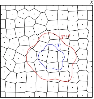
enlarged by anδ-tube. To this end, forδ >0, we defineT+δ by
T+δ:=
x∈X∃t∈T :kx−tk2≤δ ,
which impliesT ⊂T+δ⊂X, cf. Figure 4. Note that, for everyδ >0, there exists annδ ∈N
such that, for everyn≥nδ, the union of all partition setsAj, having at least one common point withT, is contained inT+δ, i.e.
∀δ >0 ∃nδ ∈N ∀n≥nδ : [
j∈JT
Aj ⊂T+δ, (19)
whereJT :={j∈ {1, . . . , mn}:Aj∩T 6=∅}. Collectively, this impliesT ⊂Sj∈JTAj ⊂T +δ for alln≥nδ. Furthermore, since every setAj is contained in a ball with radiusrn=cn−
1 βd
satisfying (5), the lowest sample sizenδ in (19) can be determined by choosing the smallest
nδ∈Nsuch thatδ ≥2rnδ, that is
nδ = &
2c
δ βd'
.
T T+δ
X
Figure 4: An input space X with a Voronoi partition as well as a subset T ⊂ X enlarged by an
δ-tube toT+δ.
Corollary 6 Let Y := [−M, M]for M >0, L:Y ×R→ [0,∞) be the least squares loss,
and P be a distribution on Rd×Y. We denote the marginal distribution of P onto Rd
by PX, write X := supp PX, and assume PX(∂X) = 0. Furthermore, let (A) and (G)
be satisfied. In addition, for an arbitrary subset T ⊂ X, we assume (T) . Moreover, let
fL,∗P:Rd→Rbe a Bayes decision function with fL,∗P∈L2(Rd)∩L∞(Rd) as well as
fL,∗P∈B2α,∞(PX|T+δ)
for α ≥ 1 and some δ > 0. Then, for all p ∈ (0,1), n ≥ nδ, τ ≥ 1, γ = (γ1, . . . , γm) ∈
(0, r]m, and λ= (λ1, . . . , λm)>0, the VP-SVM given by (3)using Hˆγ1(A1), . . . ,Hˆγm(Am),
and the loss LT satisfies
m X
j=1
λjkfDj,λj,γjk 2
ˆ
Hγj(Aj)+RLT,P(fÛD,λ,γ)− R
∗
LT,P
≤CM,α,p
X
j∈JT
λjγ−jd+
maxj∈JTγj
minj∈JTγj
d max j∈JT
γj2α+r2p
m X
j=1
λ−j1γ−
d+2p p
j PX(Aj)
p
n−1+τ n−1
with probability Pn not less than 1−e−τ, where CM,α,p > 0 is the same constant as in
Theorem 4.
Additionally, let β ≥ 2dα+ 1 as well as, for every j ∈ {1, . . . , mn}, rn, λn,j, and γn,j be
as in (16), (17), and (18), respectively, where c1, c2, c3 are user-specified positive constants
with c3≤c1. Then, for alln≥nδ=
l
2c1
δ βdm
and ξ >0, we have
RLT,P(fÛD,λ
n,γn)− R
∗
LT,P≤C
n−2α2α+d+ξ+τ n−1
with probability Pn not less than 1−e−τ, where λn := (λn,1, . . . , λn,mn), γn := (γn,1, . . . ,
Note that the assumption fL,∗P ∈ Bα2,∞(PX|T+δ) made in Corollary 6 is satisfied if,
for example, PX has a bounded Lebesgue density on T+δ, fL,∗P ∈ L∞(T+δ), and either
fL,∗P ∈ Bα2,∞(T+2δ) for α ≥ 1 or fL,∗P ∈ W2α(Te) ⊂ B2α,∞(T+2δ) for α ∈ N and a bounded Lipschitz domain Te ⊂ Rd such that T+2δ ⊂ Te. Moreover, if this density of PX is even bounded away from 0, it is well-known that the minmax rate is n−2α2α+d for α > d/2 and
target functions fL,∗P ∈ W2α(T) as well as for α > d and fL,∗P ∈ B2α,∞(T). Modulo ξ, our rate is therefore asymptotically optimal in a minmax sense on T.
Although the obtained learning rates are arbitrary close to the optimal rates, it is needless to say that the results are not fully satisfying. Indeed, an ideal result would not contain a gap of the form nξ, and a close to ideal result would at least replace the gap
nξ by a logarithmic factor. Unfortunately, even for global SVMs using Gaussian kernels, such results seem to be currently out of reach, see (Eberts and Steinwart, 2013) for the latter case. Let us briefly describe the technical obstacles. One key ingredient for both the local and the global approach are estimates on the entropy numbers ei of the embeddings id :Hγ→L2(PX) or id :Hγ→`∞(X), see Section 6 for a definition. Several such estimates
do exist. For example, Zhou (2002) and K¨uhn (2011) proved (optimal) super-polynomial estimates but unfortunately their bounds have a unfavorable dependence onγ, which makes it impossible to get arbitrarily close to the optimal rates, see e.g., (Xiang and Zhou, 2009) for a similar situation in which this problem occurs. For this reason we followed the path of (Eberts and Steinwart, 2013), in which we employ an entropy estimate of the form
ei id :Hγ→L2(PX)
≤cp,dγ−pi−
p
d, i≥1, γ∈(0,1],
where cp,d ≥ 1 is a constant only depending on p ∈ N and d. Note that this estimate is
clearly sub-optimal in i, but it has a significantly better behavior in γ compared to the above mentioned results. Now, using this entropy estimate, Eberts and Steinwart (2013) obtain an oracle inequality of the form
RL,P(fD,λ,γ)−R∗L,P≤Kp
λγ−d+γ2α+c d/p p,d γ
−d
λ2dpn
+τ
n
,
where the constant Kp is independent of γ, λ, τ, and n, and its dependence on p can be tracked, cf. (Steinwart and Christmann, 2008, p. 267). Note that for the local approach a structurally identical formula is derived implicitly in the proof of Theorem 4. Now, the rates in this paper as well as in (Eberts and Steinwart, 2013) are obtained by optimizing the right hand side with respect to bothλand γ for an arbitrarily large but fixedp. Since the resulting rates become better the larger we pick p it is tempting to considerp =pn →
4.2 Data-Dependent Parameter Selection for VP-SVMs
In the previous theorems the choice of the regularization parameters λn,1, . . . ,
λn,mn and the kernel widthsγn,1, . . . , γn,mn requires us to know the smoothness parameter
α. Unfortunately, in practice, we usually do know neither this value nor its existence. In this subsection, we thus show that a training/validation approach similar to the one examined in (Steinwart and Christmann, 2008, Chapters 6.5, 7.4, 8.2) and (Eberts and Steinwart, 2013) achieves the same rates adaptively, i.e., without knowing α. For this purpose, let Λ := (Λn) and Γ := (Γn) be sequences of finite subsets Λn⊂(0, rdn] and Γn⊂(0, rn]. For a data set D:= ((x1, y1), . . . ,(xn, yn)), we define
D1 := ((x1, y1), . . . ,(xl, yl)),
D2 := ((xl+1, yl+1), . . . ,(xn, yn)), wherel:=bn
2c+ 1 and n≥4. We further split these sets in data sets
D(1)j :={(xi, yi)∈D1:xi∈Aj}, j∈ {1, . . . , mn},
D(2)j :={(xi, yi)∈D2:xi∈Aj}, j∈ {1, . . . , mn},
and define lj := |D(1)j | for all j ∈ {1, . . . , mn} such that Pmj=1n lj = l. For every j ∈
{1, . . . , mn}, we basically useDj(1) as a training set, i.e., based onD1 in combination with
the loss functionLj :=1AjLwe compute SVM decision functions
f
D(1)j ,λj,γj := arg min
f∈Hˆγj(Aj)
λjkfk2Hˆγj(Aj)+RLj,D1(f), (λj, γj)∈Λn×Γn.
Note that f
D(1)j ,λj,γj = 0 if D (1)
j =∅. Next, for each j, we use D2 in tandem with Lj (or essentiallyD(2)j ) to determine a pair (λD2,j, γD2,j)∈Λn×Γn such that
RLj,D2
Û
f
D(1)j ,λD2,j,γD2,j
= min
(λj,γj)∈Λn×Γn RLj,D2
Û
f
D(1)j ,λj,γj
.
Finally, combining the decision functionsfD(1)
j ,λD2,j,γD2,jfor allj∈ {1, . . . , mn}, and defining λD2 := (λD2,1, . . . , λD2,mn) and γD2 := (γD2,1, . . . , γD2,mn), we obtain a function
fD1,λD2,γD2 :=
mn
X
j=1
fD(1)
j ,λD2,j,γD2,j =
mn
X
j=1
1AjfD(1)
j ,λD2,j,γD2,j,
and we call every learning method that produces these resulting decision functions
fD1,λD2,γD2 a training validation Voronoi partition support vector machine (TV-VP-SVM)
w.r.t. Λ×Γ. Moreover, we have, for λ:= (λ1, . . . , λmn) andγ := (γ1, . . . , γmn),
RL,D2
Û
fD1,λD2,γD2
=
mn
X
j=1 RLj,D2
Û
fD(1)
j ,λD2,j,γD2,j
= mn
X
j=1
min
(λj,γj)∈Λn×Γn RLj,D2
Û
f
D(1)j ,λj,γj
= min
(λ,γ)∈(Λn×Γn)mn
mn
X
j=1
RLj,D2
Û
f
D(1)j ,λj,γj
= min
(λ,γ)∈(Λn×Γn)mnRL,D2
Û
fD1,λ,γ
,
where fD1,λ,γ :=
Pmn
j=1fD(1)
j ,λj,γj with (λj, γj) ∈ Λn× Γn for all j ∈ {1, . . . , mn}. In
other words, the function fÛD
1,λD2,γD2 really minimizes the empirical risk RL,D2 w.r.t. the
validation data setD2 and the lossL, where the minimum is taken over all functionsfÛD
1,λ,γ
with (λ,γ)∈(Λn×Γn)mn.
Before we analyze the TV-VP-SVM algorithm, let us briefly discuss the computational complexity of the hyper-parameter selection step. To this end, we first note that the pa-rameter selection on, e.g., thej-th cell iscompletely independent of the parameter selection on all other cells. Maybe the easiest way to visualize this is by thinking of having two cells and candidates Λ = (λ1, . . . , λk), only. Naively, this would give the candidate set Λ×Λ for the overall hyper-parameter selection procedure. However, inspecting the candidates on the first cell, we see the same results for the candidates in Λ× {λ1} and in Λ× {λ2}since
any decision we make on the second cell does not influence our situation on the first cell. Consequently, we only need to consider the candidates Λ× {λ1}, that is the candidates in
Λ, when performing parameter selection on the first cell, and analogously we only need to consider the candidates {λ1} ×Λ for the parameter selection on the second cell. Together
this gives 2|Λ|many candidates, instead of|Λ|2 many candidates of the naive approach.
Generalizing the reasoning above tom cells and Λ×Γ, we easily see that our parameter selection strategy leads to the inspection of m× |Λ| × |Γ| many candidates. Moreover, because of the independence of all cells, we could actually perform parameter selection on the cells in parallel. Clearly such a parallel approach would be easy to implement and would have minimal synchronization and communication overhead.
The following theorem presents learning rates for the above described TV-VP-SVM.
Theorem 7 Let rn := cn
−1
βd with constants c > 0 and β > 1. Under the assumptions
of Theorem 4 we fix sequences Λ := (Λn) and Γ := (Γn) of finite subsets Λn ⊂ (0, rdn]
and Γn ⊂(0, rn] such that Λn is an (rndεn)-net of (0, rdn] and Γn is a δn-net of (0, rn] with
εn≤ n−1 and δn ≤n−
1
2+d. Furthermore, assume that the cardinalities |Λn| and |Γn| grow
polynomially in n. Then, for all ξ >0, τ ≥1, and α < β−21d, the TV-VP-SVM producing
the decision functions fD1,λD2,γD2 satisfies
Pn
RL
JT,P(fÛD1,λD2,γD2)− R
∗
LJT,P≤c
n−2α2α+d+ξ+τ n−1
≥1−e−τ,
where c >0 is a constant independent of n and τ.
Once more, we can replace the assumptionfL,∗P∈B2α,∞(PX|AT) byf
∗
L,P∈B2α,∞(PX|T+δ)
T+δ is fixed for all n ∈ N. Here, recall that fL,∗P ∈ B2α,∞(PX|T+δ) whenever PX has a
bounded Lebesgue density on T+δ, fL,∗P ∈ L∞(T+δ), and either fL,∗P ∈ B2α,∞(T+2δ) for α≥1 or fL,∗P∈W2α(Te)⊂B2α,∞(T+2δ) forα∈Nand a bounded Lipschitz domain Te⊂Rd such that T+2δ ⊂ Te. Moreover, let us assume that Te ⊇ T+δ is a bounded Lipschitz domain in Rd such that Stein’s extension operator E exists and that P is a distribution
on Rd×Y such that PX has a Lebesgue density g on T+δ with g∈ L∞(T+δ). Then, the
assumptions fL,∗P ∈Bα2,∞(Te) and fL,∗P ∈L∞(Te) yield EfL,∗P ∈B2α,∞(PX|T+δ) and EfL,∗P ∈
L2(Rd)∩L∞(Rd), see (Eberts, 2015, Corollary 3.4 and Theorem 3.2) for more details. Thus,
applying R∗L
JT,P=RLJT,P(Ef
∗
L,P) and choosingf0 :=
P
j∈JT1Aj ·(Kj ∗Ef
∗
L,P), we obtain
the same results as in Corollary 6 and Theorem 7 forn≥nδ. Obviously, the same is true, if we assume fL,∗P ∈ W2α(Te) instead of fL,∗P ∈ Bα2,∞(Te). For all these cases, note that, if PX has a Lebesgue density that is bounded away from 0 and ∞ and eitherfL,∗P∈W2α(T)
for α > d/2 or fL,∗P ∈ B2α,∞(T) for α > d, the achieved learning rate n−2α2α+d is again
asymptotically optimal moduloξ on T in a minmax sense. Here, we only derived learning rates when using the least squares loss. However, similar rates are shown by Eberts (2015, Section 9) for quantile regression using the pinball loss.
To derive the above learning rates, we need the condition α < β−21d. However, this condition restricts the set of α-values where we obtain learning rates adaptively. To be more precise, there is a trade-off between α and β. On the one hand, for small values of β
only a small number of possible values forαis covered. On the other hand, for larger values of β the set of α-values where we achieve rates adaptively is increasing but the savings in terms of computing time is decreasing.
Finally, we note that if we have a fixed computational budget in terms of RAM and/or computing time, this trade-off can be approximately resolved in the following way. First, we consider a couple of candidates for β, or the resulting number of cells m. Then, we pick a suitably sized random subset of the entire training set and build Voronoi partitions of this random subset for the different candidates. For each cell of these partitions we then estimate the computational costs and finally we pick the largest candidateβ for which the resulting partition still satisfies our computational budget. This procedure has several benefits: a) it is very cheap compared to the subsequent training and parameter selection phase,b) the choice ofβ, or m, has a clear meaning for the user,c) it approximately leads to widest adaptivity we can afford by our computational budget, and d) our experiments in the next section show that there is no significant risk for the user by focusing on the maximal computational resources.
5. Experimental Results
In this section we report a few experiments for VP-SVMs, which illustrate the influence of the chosen radius and which compare them to standard global SVMs as well as to RC-SVMs in terms of both training time and test error.
In the experiments we report here, we consider the classical covtype data set, which
Algorithm 1 Determine a Voronoi partition of the input data
Require: Input data setDX ={x1, . . . , xn}with sample sizen∈Nand some radiusr >0. Ensure: Working sets indicating a Voronoi partition of DX.
1: Pick an arbitraryz∈DX
2: Cover1 ←z
3: m←1
4: whilemaxx∈DXkx−Coverk2 > rdo
5: z←arg maxx∈DXkx−Coverk2
6: m←m+ 1
7: Coverm←z
8: WorkingSetm← ∅
9: end while
10: fori= 1 ton do
11: k←arg minj∈{1,...,m}kxi−Coverjk2
12: WorkingSetk←WorkingSetk∪ {xi}
13: end for
14: return WorkingSet1, . . . ,WorkingSetm
highly efficient SVM solvers for different loss functions based on the ideas developed by (Steinwart et al., 2011). In particular, it is easy to repeat every experiment by the current version of the code.
In order to prepare the data set for the experiments, we first merged the split raw data sets so that we obtained one data set. In a next step, we scaled the data component-wise such that all samples including labels lie in [−1,1]d+1, where d is the dimension of the input data. Finally, we generated random subsets that were afterwards randomly split into a training and a test data set. In this manner, we obtained training sets consisting of n = 1 000, 2 500, 5 000, 10 000, 25 000, 50 000, 100 000, 250 000, and 500 000 samples. The test data sets associated to the various training sets consist of ntest = 50 000 random
samples, apart from the training sets with ntrain ≤5 000, for which we tookntest = 10 000
test samples. To minimize random effects, we repeated the experiment for each setting several times. Since experiments using large data sets entail long run times, we reran every experiment using a training set of sizen≥50 000 only three times while for training sets of sizen= 10 000, 25 000 we performed ten repetitions and for smaller training sets, namely of size n= 1 000, 2 500, 5 000, even 100 runs.
To train the global SVM for sufficiently large data sets we used a professional compute server equipped with four INTEL XEON E7-4830 (2.13 GHz) 8-core processor, 256 GB RAM. In order to have comparable run times, we ran the experiments for the VP-SVMs and RC-SVMs on this machine, too. In all experiments we used eight cores to pre-compute the kernel matrix and to evaluate the final decision functions on the test set, but only one core for the actual solver.
first traversal algorithm, see (Dasgupta, 2008) and (Gonzalez, 1985) for more details. Note that this procedure induces working sets whose sizes may be considerably varying. In the case of an RC-SVM the working sets form a random partition of the training samples, where their sizes are basically equal and the number of working sets is predefined by the user. Then, for the VP-SVM- as well as for the RC-SVM-algorithm the implemented LS-solver is applied on every working set. For each working set, we randomly split the respective training data set of size ntrain in five folds to apply 5-fold cross-validation in order to deal
with the hyper-parameters λ and γ taken from an 10 by 10 grid geometrically generated in [0.001·n−train1 ,0.1]×[0.5·n−train1/d,10]. Finally, we obtain one decision function for each working set. To further process these decision functions the VP-SVM-algorithms picks exactly one decision function depending on the working set affiliation of the input value. On the contrary, the RC-SVM-algorithm simply takes the average of all the decision functions. Moreover, the computed decision functions are clipped at ±1. Altogether, note that the usual LS-SVM-algorithm can be interpreted as special case of both the VP-SVM- and the RC-SVM-algorithm using one working set.
The results, which are displayed in Figure 5, can be quickly summarized: Not surpris-ingly, smaller radii for the VP-SVM lead to less crowded cells, which in turn reduces the training time significantly. In addition, the VP-SVM is, unlike the global SVM, not af-fected by the amount of available memory, so that runs with more than 100.000 samples, which would require kernel matrix caching for the global SVM, are still very feasible for the VP-SVM. Despite these advantages in terms of required computational resources, however, the test errors of the VP-SVM are only a bit worse than those of the global SVM. More-over, the test errors become slightly better with increasing radii, so that there is a clear trade-off between computational resources and test accuracy as discussed in the previous section. When comparing the RC-SVM with the global SVM, we see, not surprisingly, the same computational advantages, but the test errors become significantly worse. As a consequence, the VP-SVM clearly outperforms the RC-SVM in terms of test errors, when both approaches have about the same training time. In this respect we also like to mention that in terms of test time, the VP-SVM was significantly faster than the RC-SVM, simply because for the VP-SVM each decision function evaluation only requires the support vector of the corresponding cell, whereas the final decision function of the RC-SVM requires all support vectors. See (Eberts and Steinwart, 2014) for details.
6. Proofs
This section is dedicated to prove the results of the previous sections.
We begin by recalling the definition of entropy and covering numbers. To this end, let (T, d) be a metric space. Then, thei-th (dyadic) entropy number of T is
ei(T, d) := inf (
ε >0 :∃s1, . . . , s2i−1 ∈T such that T ⊂ 2i−1
[
j=1
B(sj, ε) )
,
0
200
400
600
sample size
tr
aining time [sec]
1000 2500 5000 10000
nr of ws = 5 nr of ws = 10 nr of ws = 50 nr of ws = 100
(a) Average training time of the various RC-SVMs for ntrain≤10 000
0
20000
40000
60000
sample size
tr
aining time [sec]
5000 25000 100000 500000
(b) Average training time of the various RC-SVMs for ntrain≥5 000
0.2
0.4
0.6
0.8
sample size
test error
1000 5000 25000 500000
(c) Average empirical risk of the various RC-SVMs
0
20
40
60
80
100
120
sample size
tr
aining time [sec]
1000 2500 5000 10000
VP−SVM using radius = 2 radius = 3 radius = 4 radius = 5
(d) Average training time of the various VP-SVMs for ntrain≤10 000
0
5000
15000
25000
35000
sample size
tr
aining time [sec]
5000 25000 100000 500000
(e) Average training time of the various VP-SVMs for ntrain≥5 000
0.2
0.3
0.4
0.5
0.6
0.7
sample size
test error
1000 5000 25000 500000
(f) Average empirical risk of the various VP-SVMs
0
20
40
60
80
100
120
140
sample size
tr
aining time [sec]
1000 2500 5000 10000
LS−SVM VP−SVM (radius = 2) RC−SVM (50 working sets) RC−SVM (100 working sets)
(g) Average training time of LS-, VP-, and RC-SVMs for ntrain≤10 000
0
5000
10000
15000
sample size
tr
aining time [sec]
5000 25000 100000 500000
(h) Average training time of LS-, VP-, and RC-SVMs for ntrain≥5 000
0.2
0.3
0.4
0.5
0.6
0.7
sample size
test error
1000 5000 25000 500000
(i) Average empirical risk of LS-, VP-, and RC-SVMs
Figure 5: Average training time and test error of LS-, VP-, and RC-SVMs for the real-world data
covtypedepending on the training set sizentrain= 1 000, . . . ,500 000. Subfigures (a)–(c)
show the results for RC-SVMs using different numbers of working sets and Subfigures (d)–(f) illustrate the results for VP-SVMs using various radii. At the bottom, Subfigures (g)–(i) contain the average training times and the average test errors of the LS-SVM, one VP-SVM and two RC-SVMs. Here, the VP-SVM is the one which trains fastest for
ntrain = 500 000 and the two RC-SVMs are those which achieve forntrain= 500 000 roughly
the same training time as the chosen VP-SVM. Here, note that, for ntrain = 10 000, the
Similarly, theε-covering number ofT is defined by
N(T, d, ε) := inf (
n≥1 :∃s1, . . . , sn∈T such that T ⊂ n [
i=1
Bd(si, ε) )
,
and again, this definition can be applied to bounded linear operators S : E → F by considering the setSBE. Moreover, every subsetS ⊂T for which for allt∈T there exists an s∈S withd(s, t)≤εis called an ε-net ofT. Consequently,N(T, d, ε) is the size of the smallest ε-net ofT. Recall that entropy and covering numbers are in some sense inverse to each other. To be more precise, for all constants a >0 and q >0, the implication
ei(T, d)≤ai−1/q, i≥1 =⇒ lnN(T, d, ε)≤ln(4)
a
ε q
, ∀ε >0 (20)
holds by (Steinwart and Christmann, 2008, Lemma 6.21). Additionally, (Steinwart and Christmann, 2008, Exercise 6.8) yields the opposite implication, namely
lnN(T, d, ε)<a ε
q
, ε >0 =⇒ ei(T, d)≤31/qai−1/q, ∀ i≥1. (21) With these preparations, we can now prove Lemma 1, which relates the radius r of a coverBr(z1), . . . , Br(zm) ofB`d
2 ⊃Xdefined by (4) with the numbermof centersz1, . . . , zm. Proof [of Lemma 1] It is easy to show that N(cB`d
2, `
d
2, r) = N(B`d 2, `
d
2,rc) holds for all
r, c >0. Moreover, applying Proposition 1.1 of (Temlyakov, 2013) yields
˜
r−d≤ N(B`d 2, `
d
2,r˜)≤
1 +2 ˜
r d
, ˜r∈(0,1].
Consequently, we can find a cover (Br(zj))j=1,...,m of X⊂cB`d
2 with centers zj ∈cB`d2 and
radiusr ≤csuch that
r
c −d
≤m≤
1 +2c
r d
.
Since r≤c, we thus have r ≤(r+ 2c)m−1d ≤3cm− 1 d
Next, we consider a lemma that is part of our construction of the partition (Aj)j of X.
Lemma 8 Let (A0j)j=1,...,m be a partition of B`d
2 such that
˚
A0j 6=∅ as well as A˚0j =A0j for
every j ∈ {1, . . . , m}. Let X be some closed subset of B`d
2 such that
˚
X 6= ∅ and X˚ = X.
Without loss of generality we further assume that there is anm0 ≤m such thatA0j∩X˚6=∅
for all j ∈ {1, . . . , m0} and A0j ∩X˚ = ∅ for all j ∈ {m0+ 1, . . . , m}. Then, we define
A00j :=A0j ∩X˚ for all j ∈ {1, . . . , m0}. Moreover, let (Aj)j=1,...,m0 be a partition ofX with
Proof Let us assume that there is anj∈ {1, . . . , m0}with ˚A00j =∅. By our assumption we then knowA00j =A0j∩X˚=6 ∅, i.e., there exists some x∈A0j∩X˚. Since
∅= ˚A00j = interior(A0j∩X˚) = ˚A0j∩interior ˚X = ˚A0j ∩X ,˚
where we used the notation interiorB := ˚B, it immediately follows thatx∈∂Aj0 ⊂A0j = ˚A0j.
Hence, there exists a sequence (xn)n ⊂ A˚0j such that xn n
→∞
−−−→ x. On the other hand,
x∈A00j ⊂X˚together with the fact that ˚X is open, givesxn∈X˚for all sufficiently large n.
For such an n, we obtain xn ∈A˚0j∩X˚= ˚A00j, which contradicts the assumed ˚A00j =∅. The
second assertion follows from ˚A00j ⊂A˚j.
Next, let us consider a crucial property of the risk of functions contained in a joined RKHS.
Lemma 9 Let P be a distribution on X ×Y and L : X ×Y ×R → [0,∞) be a loss
function. ForA, B⊂X such that A∪B =X andA∩B =∅, define loss functionsLA, LB:
X ×Y ×R → [0,∞) by LA(x, y, t) = 1A(x)L(x, y, t) and LB(x, y, t) = 1B(x)L(x, y, t),
respectively. Furthermore, let fA :X →R as well as fB :X → R be measurable functions
and f :X → R be defined by f(x) =1A(x)fA(x) +1B(x)fB(x) for all x ∈ X. Then, we
have
RL,P(f) =RLA,P(fA) +RLB,P(fB).
as well as
RL,P(f)− R∗L,P= RLA,P(fA)− R
∗
LA,P
+ RLB,P(fB)− R
∗
LB,P
.
Proof Simple transformations usingA∪B =X and A∩B=∅show
RL,P(f) =
Z
X×Y
L(x, y,1A(x)fA(x) +1B(x)fB(x))dP(x, y)
= Z
X×Y
1A(x)L(x, y, fA(x)) +1B(x)L(x, y, fB(x))dP(x, y)
=RLA,P(fA) +RLB,P(fB).
The second assertion follows immediately.
6.1 Some General Estimates on Entropy Numbers