The em Algorithm for Kernel Matrix Completion with Auxiliary Data

The em Algorithm for Kernel Matrix Completion

with Auxiliary Data

Koji Tsuda [email protected]

Max Planck Institute for Biological Cybernetics 72076 T¨ubingen, Germany; and

AIST Computational Biology Research Center Tokyo, 135-0064, Japan

Shotaro Akaho [email protected]

AIST Neuroscience Research Institute Tsukuba, 305-8568, Japan

Kiyoshi Asai [email protected]

Department of Computational Biology Graduate School of Frontier Science University of Tokyo

Kashiwa, 277-8562, Japan; and

AIST Computational Biology Research Center Tokyo, 135-0064, Japan

Editor: Chris Williams

Abstract

In biological data, it is often the case that observed data are available only for a subset of samples. When a kernel matrix is derived from such data, we have to leave the entries for unavailable samples as missing. In this paper, the missing entries are completed by exploiting an auxiliary kernel matrix derived from another information source. The parametric model of kernel matrices is created as a set of spectral variants of the auxiliary kernel matrix, and the missing entries are estimated by fitting this model to the existing entries. For model fitting, we adopt the em algorithm (distinguished from the EM algorithm of Dempster et al., 1977) based on the information geometry of positive definite matrices. We will report promising results on bacteria clustering experiments using two marker sequences: 16S and gyrB.

Keywords: Information geometry, em algorithm, Kernel matrix completion, Bacteria clustering

1. Introduction

In kernel machines such as support vector machines (SVM) (Sch¨olkopf and Smola, 2002), objects are repre-sented as a kernel matrix, where n objects are reprerepre-sented as an n×n positive semidefinite matrix. Essentially

the(i,j)entry of the kernel matrix describes the similarity between i-th and j-th objects. Due to positive semidefiniteness, the objects can be embedded as n points in an Euclidean feature space such that the inner product between two points equals to the corresponding entry of kernel matrix. This property enables us to apply diverse learning methods (for example, SVM or kernel PCA) without explicitly constructing a feature space (Sch ¨olkopf and Smola, 2002).

impossible without additional information. So we make use of a parametric model of admissible matrices, and estimate missing entries by fitting the model to existing entries.

In this scheme, it is important to define a parametric model appropriately. For example, Graepel (2002) used the set of all positive definite matrices as a model. Although this model worked well when only a few entries are missing, this model is too general for our cases where whole columns and rows are missing. Thus we need another information source for constructing a parametric model. Fortunately, in biological data, it is common that one object is described by two or more representations. For example, genes are represented by gene networks and gene expression arrays at the same time (Vert and Kanehisa, 2003). Also a bacterium is represented by several marker sequences (Yamamoto et al., 2000). In this paper, we assume that auxiliary data are available from another information source. From the auxiliary data, a complete kernel matrix called the auxiliary matrix is derived and a parametric model is created by giving perturbations to this matrix. When creating a parametric model of admissible matrices from an auxiliary matrix, one typical way is to define the parametric model as all spectral variants1_{which have the same eigenvectors but different}

eigenvalues (Cristianini et al., 2002). When several auxiliary matrices are available, the weighted sum of these matrices would be a good parametric model as well (Lanckriet et al., 2002).

In order to fit a parametric model, the distance between two matrices has to be determined. A common way is to define the Euclidean distance between matrices (for example, the Frobenius norm) and make use of the Euclidean geometry. Recently Vert and Kanehisa (2003) tackled with the incomplete matrix approxi-mation problem by means of kernel CCA. Also Cristianini et al. (2002) proposed a similarity measure called “alignment”, which is basically the cosine between two matrices. In contrast that their methods are based on the Euclidean geometry, this paper will follow an alternative way: we will define the Kullback-Leibler (KL) divergence between two kernel matrices and make use of the Riemannian information geometry (Ohara et al., 1996). The KL divergence is derived by relating a kernel matrix to a covariance matrix of Gaussian distribution. The primal advantage is that the KL divergence allows us to use the em algorithm (Amari, 1995) to approximate an incomplete kernel matrix. The e and m steps are formulated as convex program-ming problems, and moreover they can be solved analytically when spectral variants are used as a parametric model.

We performed bacteria clustering experiments using two marker sequences: 16S and gyrB (Yamamoto et al., 2000). We derived the incomplete and auxiliary kernel matrices from gyrB and 16S, respectively. As a result, even when 50% of columns/rows are missing, the clustering performance of the completed matrix was better than that of the auxiliary matrix, which illustrates the effectiveness of our approach in real world problems.

This paper is organized as follows: Section 2 introduces the information geometry to the space of positive definite matrices. Based on geometric concepts, the em algorithm for matrix completion is presented in Section 3, where detailed computations are deferred in Section 4. In Section 5, the matrix completion problem is formulated as statistical inference and the equivalence between the em and EM algorithms (Dempster et al., 1977) is shown. Then the bacteria clustering experiment is described in Section 6. After seeking for possible extensions in Section 7, we conclude the paper in Section 8.

2. Information Geometry of Positive Definite Matrices

We first explain how to introduce the information geometry (Amari and Nagaoka, 2001) in the space of positive definite matrices. Let us define the set of all d×d positive definite matrices as

P

. The first step is to relate a d×d positive definite matrix P∈

P

to the Gaussian distribution with mean 0 and covariance matrix

P:

p(x|P) = 1

(2π)d/2_|P|1/2exp(−

1 2x

>_P−1_{x). (1)}

It is well known that the Gaussian distribution belongs to the exponential family. The canonical form of an exponential family distribution is written as

p(x|θ) =exp(θ>r(x)−ψ(θ)),

where r(x)is the vector of sufficient statistics,θis the natural parameter andψ(θ)is the normalization factor. When (1) is rewritten in the canonical form, we have the sufficient statistics as

r(x) =−

1 2x

2 1,...,1

2x

2

d,x1x2,...,xd−1xd

>

,

and the natural parameter as

θ= [P−1]11,...,[P−1]dd,[P−1]12,...,[P−1]d−1,d

>_,

where[M]i j denotes the(i,j)entry of matrix M. The natural parameterθprovides a coordinate system to specify a positive definite matrix P, which is called theθ-coordinate system (or the e-coordinate system). On the other hand, there is an alternative representation for the exponential family. Let us define the mean of

ri(x)asηi: For example, when ri(x) =xsxt,

ηi=

Z

xsxtp(x|θ)dx=Pst.

This new set of parametersηi provides another coordinate system, calledη-coordinate system (or the m-coordinate system):

η= (P11,...,Pdd,P12,...,Pd−1,d)>.

Let us consider the following curveθ(t)connecting two pointsθ1andθ2linearly inθcoordinates:

θ(t) =t(θ2−θ1) +θ1.

When written is the matrix form, this reads

P−1(t) =t(P₂−1−P₁−1) +P₁−1.

This curve is regarded as a straight line from the exponential viewpoint and is called an exponential geodesic or e-geodesic. In particular, each coordinate curveθi=t,θj=cj (j6=i)is an geodesic. When the e-geodesic between any two points in a manifold

S

⊆

P

is included in

S

, the manifold

S

is said to be e-flat. On the other hand, the mixture geodesic or m-geodesic is defined as

η(t) =t(η₂−η1) +η1.

In the matrix form, this reads

P(t) =t(P2−P1) +P1.

When the m-geodesic between any two points in

S

is included in

S

, the manifold

S

is said to be m-flat. In information geometry, the distance between probability distributions is defined as the Kullback-Leibler divergence (Amari and Nagaoka, 2001):

KL(p,q) = Z

p(x)logp(x)

q(x)dx.

By relating a positive definite matrix to the covariance matrix of Gaussian (1), we have the Kullback-Leibler (KL) divergence for two matrices P,Q:

KL(P,Q) =tr(Q−1P) +log det Q−logdet P−d.

With respect to a manifold

S

⊆

P

and a point P∈

P

, the projection from P to

S

is defined as the point in

S

• e-projection: Q∗=argmin_Q∈SKL(Q,P).

• m-projection: Q∗=argmin_Q∈SKL(P,Q).

It is proved that the m-projection to an e-flat submanifold is unique, and e-projection to an m-flat manifold is unique (Amari and Nagaoka, 2001). This uniqueness property means that the corresponding optimization problem is convex and so the global optimal solution is easily obtained by any reasonable method.

3. Completion of an Incomplete Kernel Matrix

In this section, we describe the em algorithm to complete an incomplete kernel matrix. Let x1,...,x_`∈

X

be the set of samples of interest. In supervised learning cases, this set includes both training and test sets, thus we are considering the transductive setting (Vapnik, 1998). Let us assume that the data is available for the first n samples, and unavailable for the remaining m :=`−n samples. Denote by KIan n×n kernel matrix, which is derived from the data for the first n samples. Then, an incomplete kernel matrix is described as

D=

KI Dvh

D>_vh Dhh

, (2)

where Dvh is an n×m matrix and Dhhis an m×m symmetric matrix. Since D has missing entries, it cannot be presented as a point in

P

. Instead, all the possible kernel matrices form a manifold

D

={D|Dvh∈ℜn×m, Dhh∈ℜm×m, Dhh=D>hh, D0},

where D0 means that D is positive definite. We call it the data manifold as in the conventional EM algorithm (Ikeda et al., 1999). It is easy to verify that

D

is an m-flat manifold; hence, the e-projection to

D

is unique.

Next let us define the parametric model to approximate D. Here the model is derived as the spectral variants of KB, which is an`×`auxiliary kernel matrix. Let us defineλi and vi as the i-th eigenvalue and eigenvector of KB, respectively.2Then KBis decomposed as follows:

KB=

`

∑

i=1

λiviv>i .

Define

Mi=viv>i , (3)

then all the spectral variants are represented as3

M

={M|M= `

∑

j=1

βjMj, β∈ℜ`, M0}.

We call it the model manifold (Ikeda et al., 1999). Since the eigenvectors{vi}`_i=1are orthonormal,

M

can be reparametrized as follows:

M

={M|M= ( `

∑

j=1

bjMj)−1, b∈ℜ`, M0}, (4)

where bj=1/βj. It is easily seen that the manifold

M

is e-flat and m-flat at the same time. Such a manifold is called dually-flat.

2. When`is large, the minor eigenvalues of KBmay be extremely small and the numerical computation of eigenvectors could be

instable. For stabilizing eigenvectors, it is effective to add a small positive constant to all the diagonal elements.

e

m

e

e

m

m

D

M

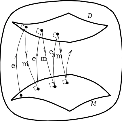
Figure 1: Information geometric picture of the em algorithm. The data manifold

_D

corresponds to the set of all completed matrices, whereas the model manifold

_M

corresponds to the set of all spectral variants of an auxiliary matrix. The nearest points are found by gradually minimizing the KL divergence by repeating e and m projections.

Our approximation problem is formulated as finding the nearest points in two manifolds: Find D∈

D

and

M∈

M

to minimize KL(D,M). In geometric terms, this problem is to find the nearest points between e-flat and m-flat manifolds. It is well known that such a problem is solved by an alternating procedure called the

em algorithm (Amari, 1995). The em algorithm gradually minimizes the KL divergence by repeating e-step

and m-step alternately (Figure 1).

In the e-step, the following optimization problem is solved with fixing M: Find D∈

D

that minimizes

KL(D,M). This is rewritten as follows: Find Dvhand Dhhthat minimize

Le=tr(DM−1)−log det D, (5)

subject to the constraint that D0. As indicated by information geometry, this is a convex problem, which can readily be solved by any reasonable optimizer. Moreover the solution is obtained in a closed form: Let us partition M−1as

M−1=

Svv Svh

S>_vh Shh

. (6)

The solution of (5) is described as

Dvh = −KISvhS−1hh, (7)

Dhh = S−1_hh +S_hh−1SvhKISvhS−1_hh. (8)

The derivation of (7) and (8) will be described in Section 4.1.

In the m-step, the following optimization problem is solved with fixing D: Find M∈

M

that minimizes

KL(D,M). This is rewritten as follows: Find b∈ℜ`that minimizes

Lm=

`

∑

j=1

bjtr(MjD)−log det(

`

∑

j=1

subject to the constraint that M0. When{Mj}`j=1are defined as (3), the closed form solution of (9) is

obtained as

bi=1/tr(MiD), i=1,...,`. (10)

The derivation of (10) will be described in Section 4.2.

4. Computing Projections

This section presents the derivation of e and m-projections in detail.

4.1 e-projection

In the following, we will derive the e-projection of M as (7) and (8). The optimization problem (5) is firstly solved without regarding the constraint D0, and then the solution is verified to satisfy the constraint. It is well known that the log determinant of a partitioned matrix is described as

log det D=log det KI+log det(Dhh−D>vhKI−1Dvh).

Thus, Lein (5) is rewritten as follows:

Le = tr(DM−1)−log det D

= tr(DM−1)−log det KI−log det(Dhh−D>vhKI−1Dvh). When we partition M−1as (6), it turns out that

Le=tr(KISvv) +2 tr(DvhSvh) +tr(DhhShh)−log det KI−log det(Dhh−D>vhKI−1Dvh). (11)

The saddle point equation with respect to Dhhis obtained as

∂Le

∂Dhh =

Shh−(Dhh−Dvh>KI−1Dvh)−1, (12)

because_∂∂_Clog detC=C−1for any symmetric matrix C. Solving (12) with respect to Dhh, we have

Dhh=S−1_hh +D>vhKI−1Dvh. (13)

Substituting (13) into (11), we have

Le=tr(KISvv) +2 tr(DvhSvh) +tr(I+ShhD>vhKI−1Dvh)−log det KI−log det Shh.

Now the saddle point equation with respect to Dvhis obtained as

∂Le

∂Dvh =

2Svh+2KI−1DvhShh=0.

Solving this equation, we have the solution (7) for Dvh. By substituting (7) into (13), we have the solution (8) for Dhh.

Next, let us verify that the solution D is positive definite (D0), that is,

c>Dc>0, (14)

for any c∈ℜ`, c6=0. The left hand side of (14) is written as

c>Dc=

c1

c2

_>

KI Dvh

D>_vh Dhh

c1

c2

.

By using the relation (13), we have the following:

c>Dc=kK_I1/2c1−KI−1/2Dvhc2k2+c2S−1hhc2. (15)

4.2 m-projection

Here we will show the derivation of the m-projection (10). Firstly let us derive the solution b to minimize

Lm=

`

∑

j=1

bjtr(MjD)−log det(

`

∑

j=1

bjMj).

without the constraint M0. Since∂log det Q−1/∂Q=Q, the saddle point equations are described as

tr(Mi(

`

∑

j=1

bjMj)−1) =tr(MiD), i=1,...,`. (16)

Remembering that Mj=vjv>j, we have

(

∑

` j=1

bjMj)−1=

`

∑

j=1

1

bj

vjv>j.

The left hand side of (16) is rewritten as

tr(Mi(

`

∑

j=1

bjMj)−1) =tr(viv>i

`

∑

j=1

1

bj

vjv>j).

Since v>_i vj=0(i6=j), we have the following:

tr(Mi(

`

∑

j=1

bjMj)−1) =tr( 1

bi

viv>i ) = 1

bi.

Therefore, the solution of (16) is analytically obtained as

bi=1/tr(MiD) =

v>_i Dvi

−1

, i=1,...,`.

When D is positive definite, we have v>_i Dvi>0 and thus bi>0. Since{b−1i }`i=1correspond to the eigenvalues

of M, M is proven to be positive definite.

We have shown that the m-projection is obtained analytically when the model manifold corresponds to spectral variants of a matrix. However, it is not always the case. For example, consider we have c auxiliary matrices N1,...,Ncand the model manifold is constructed as the harmonic mixture of them:

M

={M|M= (

c

∑

j=1

bjNj)−1, b∈ℜc, M0}. (17)

This is an e-flat manifold, so the optimization problem is convex, but the analytical solvability depends on geometric properties of auxiliary matrices{Ni}ci=1(Ohara, 1999). We will briefly discuss this issue in the

Appendix.

5. Relation to the EM algorithm

distributions. Nevertheless it would be meaningful to rewrite our method in terms of statistical concepts for establishing connections to other methods such as the probabilistic PCA (Tipping and Bishop, 1999), the Gaussian processes (Williams, 1999, Csat´o and Opper, 2002) and the Bayesian covariance kernel (Seeger, 2002).

Let v and h be the n and m dimensional visible and hidden variables. From observed data,4the covariance matrix of v is known as

Eo[vv>] =KI,

where Eodenotes the expectation with respect to observed data. However, we do not know the covariances

Dvh=Eo[vh>]and Dhh=Eo[hh>]. Our purpose is to obtain the maximum likelihood estimate of parameter

b of the following Gaussian model:

p(v,h|b) = 1

(2π)d/2|_M|1/2exp −

1 2

v h

_>

M−1

v h

! ,

where M is described as (4).

In the course of maximum likelihood estimation, we have to estimate the observed covariances Dvhand

Dhhin an appropriate way. The EM algorithm consists of the following two steps.

• E-Step: Fix b and update Dvhand Dhhby conditional expectation. • M-Step: Fix D and update b by maximum likelihood estimation.

It is shown that the likelihood of observed data increases monotonically by repeating these two steps (Demp-ster et al., 1977).

The M-step maximizes the likelihood, which is easily seen to be equivalent to minimizing the KL diver-gence (Amari, 1995). So the M-step is equivalent to the m-step (9). However, the equivalence between E-step and e-step is not obvious, because the former is based on conditional expectation and the latter minimizes the KL divergence. In the E-step, the covariance matrices are computed from the conditional distribution described as

p(h|v,b) = 1

(2π)m/2_|S−1 hh|1/2

exp

−1

2(h+S

−1

hhSvh>v)>Shh(h+S−1hhS>vhv)

,

where S matrices are derived as (6). Taking expectation with this distribution, we have

Eb[vh>|v] = −vv>SvhS_hh−1,

Eb[hh>|v] = S_hh−1+S−1_hhS>vhvv>SvhS−1_hh.

Then the covariance matrices are estimated as

Dvh=EoEb[vh>|v] = −KISvhShh−1,

Dhh=EoEb[hh>|v] = Shh−1+S−1hhS>vhKISvhS−1hh.

Since these solutions are equivalent to (7) and (8), respectively, the E-step is shown to be equivalent to the

e-step in this case. It is well known that the conditional expectation leads to the minimization of the KL

divergence in most cases (Csisz´ar and Tusnady, 1984, Neal and Hinton, 1999). However, there are special cases that the EM and em algorithms are different (Amari, 1995).

6. Bacteria Classification Experiment

In this section, we perform unsupervised classification experiments for bacteria based on two marker se-quences: 16S and gyrB. Basically we would like to identify the genus of a bacterium by means of extracted entities from the cell. It is known that several specific proteins and RNAs can be used for genus identifi-cation (Kasai et al., 1998). Among them, we especially focus on 16S rRNA and gyrase subunit B (gyrB) protein. 16S rRNA is an essential constituent in all living organisms, and the existence of many conserved regions in the rRNA genes allows the alignment of their sequences derived from distantly related organisms, while their variable regions are useful for the distinction of closely related organisms. GyrB is a type II DNA topoisomerase which is an enzyme that controls and modifies the topological states of DNA supercoils. This protein is known to be well preserved over evolutional history among bacterial organisms thus is supposed to be a better identifier than the traditional 16S rRNA (Kasai et al., 1998). Notice that 16S is represented as a nucleotide sequence with 4 symbols, and gyrB is an amino acid sequence with 20 symbols. Since gyrB has been found to be useful more recently than 16S (Yamamoto et al., 2000), gyrB sequences are available only for a limited number of bacteria. Thus, it is considered that gyrB is more “expensive” than 16S.

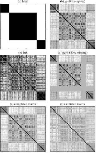
Our dataset has 52 bacteria of three genera (Corynebacterium: 10, Mycobacterium: 31, Rhodococcus: 11), each of which has both 16S and gyrB sequences. For simplicity, let us call these genera as class 1-3, respectively. For 16S and gyrB, we computed the second order count kernel, which is the dot product of bimer counts (Tsuda et al., 2002). Each kernel matrix is normalized such that the norm of each sample in the feature space becomes one. The kernel matrices of gyrB and 16S can be seen in Figure 2 (b) and (c), respectively. For reference, we show an ideal matrix as Figure 2 (a), which indicates the true classes. In our scenario, for a considerable number of bacteria, gyrB sequences are not available as in Figure 2 (d). We will complete the missing entries by the em algorithm with the spectral variants of the 16S matrix. When the em algorithm converges, we end up with two matrices: the completed matrix on data manifold

_D

and the

estimated matrix on model manifold

_M

. The completed and estimated matrices are shown in Figure 2 (e)

and (f), respectively. These two matrices are in general not the same, because the two manifolds may not have intersection.

In order to evaluate the quality of completed and estimated matrices, K-means clustering is performed in the feature space of each kernel. Clustering is repeated 20 times with different initial centers selected ran-domly from the samples. We have chosen the clustering result with the smallest squared error. In evaluation, we use the mutual information score between the obtained clusters and the true classes (Vaithyanathan and Dom, 1999).5Let U1,...,Ucbe the obtained clusters and T1,...,Tcbe the true classes. Let pi jbe the fraction of the samples which belong to both Uiand Tj. Also let pi.and p.j be the fractions of the samples in Uiand

Tj, respectively. The mutual information is defined as

c

∑

i=1 c

∑

j=1

pi jlog

pi j

pi.pj..

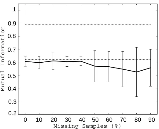
The clustering experiment is performed by randomly removing samples from the gyrB data. The ratio of missing samples is changed from 0% to 90%. The mutual information scores of completed and estimated matrices averaged over 20 trials are shown in Figures 3 and 4, respectively. Comparing the two matrices, the estimated matrix performed significantly worse than the complete matrix. It is because the completed matrix maintains existing entries unchanged, and so the class information in the gyrB matrix is well preserved. We especially focus on the comparison between the completed matrix and the 16S matrix, because there is no point in performing the em algorithm when the 16S matrix works better than the completed matrix. According to the plot, the mutual information score of the completed matrix was larger than that of the 16S matrix up to 50% missing ratio. It implies that the matrix completion is meaningful even in quite hard situations—50% sample loss implies 75% loss in entries. This result encourages us (and hopefully readers) to apply the em algorithm to other data such as gene networks (Vert and Kanehisa, 2003).

(a) Ideal (b) gyrB (complete)

(c) 16S (d) gyrB (20% missing)

(e) completed matrix (f) estimated matrix

0.2 0.3 0.4 0.5 0.6 0.7 0.8 0.9 1

Mutual Information

0 10 20 30 40 50 60 70 80 90

Missing Samples (%)

Figure 3: Clustering performance of the completed matrix. The solid curve shows the averaged mutual information score of the completed matrix, and the error bar describes the standard deviation. The upper and lower flat lines show the mutual information scores of the complete gyrB and 16S kernel matrices, respectively.

0.2 0.3 0.4 0.5 0.6 0.7 0.8 0.9 1

Mutual Information

0 10 20 30 40 50 60 70 80 90

Missing Samples (%)

7. Possible Extension

As we related the em algorithm to maximum likelihood inference in Section 5, it is straightforward to gener-alize it to the maximum a posteriori (MAP) inference or more generally the Bayes inference (Robert, 1994). For example, we are going to modify the em algorithm to obtain the MAP estimate. The MAP estimation amounts to minimizing the KL divergence penalized by a prior,

KL(D,M)−logπ(M), D∈

D,

M∈

_M

,

whereπ(M)is a prior distribution for M. Since the additional term−logπ(M)depends only M, only the

m-step is changed so as to minimize the above objective function with respect to M.

Let us give a simple example of the MAP estimation in the spectral variants case. In Bayesian infer-ence, it is common to take a conjugate prior, so that the posterior distribution remains as a member of the exponential family. Since the model parameter b is related to a covariance matrix, we choose the Gamma distribution, which works as a conjugate prior for the variance of Gaussian distribution (Robert, 1994). The prior distribution is defined independently for each bjas

π(bj;νj,αj) = 1

Γ(νj)αν_jj exp

−bj

αj+ (

νj−1)log bj

,

whereνjandαjdenote hyperparameters, by which the mean and the variance are specified by E(bj) =αjνj and V(bj) =α2jνj, respectively. The m step for the MAP estimation is to minimize

LMAP_m =Lm−

`

∑

j=1

logπ(bj;νj,αj),

which leads to the equation

tr(Mi(

`

∑

j=1

bjMj)−1) +

νi−1

bi =

tr(MiD) + 1

αi,

i=1,...,`.

In the spectral variants case, the left hand side is reduced to νi/bi, thus we obtain the MAP solution in a closed form as

bi=

νi tr(MiD) +1/αi,

i=1,...,`.

When we construct the spectral variants model, the eigenvaluesλj of the auxiliary matrix KBare dis-carded. It may cause the undesirable solution, whenλjcarries significant information. To solve the problem, we can use the MAP estimation by constraining the parameter values around the corresponding eigenvalues. A typical choice is thatνjis set to a certain constantν0andαjis determined so that the mean valueαjνjis

λj, i.e.αj=λj/ν0.

8. Conclusion

In Section 5, we related matrix completion to statistical inference. In future works, it would be interesting to involve advanced methods in statistical inference, such as generalized EM (Dempster et al., 1977) and variational Bayes (Attias, 1999). Also we are looking forward to apply our method to diverse kinds of real data which are not limited to bioinformatics.

Acknowledgments

The authors gratefully acknowledge that the bacterial gyrB amino acid sequences are offered by courtesy of Identification and Classification of Bacteria (ICB) database team of Marine Biotechnology Institute, Ka-maishi, Japan. The authors would like to thank T. Kin, Y. Nishimori, T. Tsuchiya and J.-P. Vert for fruitful discussions. Many thanks to the anonymous reviewers for their helpful comments.

Appendix A. Analytical Solvability of the m-step

In this appendix, we discuss the solvability of the m-step. The left hand side of (16) is the m-coordinate of the submanifold

M

, while bjdenote the e-coordinate of

M

. The e-coordinate and m-coordinate are connected by the Legendre transform (Amari and Nagaoka, 2001). In the mother manifold

P

, the Legendre transform is easily obtained as the inverse of the matrix. In the submanifold

M

of

P

, however, it is difficult to obtain the Legendre transform in general. The difficulty is caused by the difference of geodesics defined in

M

and

P

. When the geodesic defined by a coordinate system of a submanifold

S

⊆

P

coincides with the geodesic defined by the corresponding global coordinate system of

P

, the submanifold is called autoparallel. In our case,

M

is autoparallel for the e-coordinate, but it is not always autoparallel for the m-coordinate. When the submanifold is autoparallel for the both coordinate systems, the submanifold is called doubly autoparallel.

Let us consider when a submanifold becomes doubly autoparallel. To begin with, let us define the product

∗between two d×d symmetric matrices X,Y∈Sym(d),

X∗Y =1

2(XY+Y X). (18)

The algebra equipped with the usual matrix sum and the product (18) is called the Jordan algebra of the vector space of Sym(d). The following theorem provides the necessary and sufficient condition for a submanifold to be doubly autoparallel (Ohara, 1999).

Theorem 1 Assume the identity matrix I is an element of the submanifold

M

. Then

M

is doubly autoparallel if and only if the tangent space of

M

is a Jordan subalgebra of Sym(d).

Ohara (1999) has also shown that, if

M

is doubly autoparallel, the m-projection can be solved analytically, that is, the optimal solution is obtained by one Newton step.

For example, let us consider a submanifold

M

⊆

P

is determined as (17), the m-coordinate on

M

is defined by

ηi=tr(Ni( c

∑

j=1

bjNj)−1).

Although the m-projection onto

M

from D is explicitly given byηi=tr(NiD), the Legendre transform fromηi to the e-coordinate bjis not obtained in a closed form in general. However, if Niforms the Jordan subalgebra, that is, the following holds for all i,j:

Ni∗Nj∈span({N1,...,Nc}),

then M is doubly autoparallel and the Legendre transform can be obtained in a closed form. In the spectral variants case that we have considered, Ni=viv>i and

Ni∗Nj=0∈span({N1,...,Nc}).

References

S. Amari. Information geometry of the EM and em algorithms for neural networks. Neural Networks, 8(9): 1379–1408, 1995.

S. Amari and H. Nagaoka. Methods of Information Geometry, volume 191 of Translations of Mathematical

Monographs. American Mathematical Society, 2001.

H. Attias. Inferring parameters and structure of latent variable models by variational Bayes. In Uncertainty in

Artificial Intelligence: Proceedings of the Fifteenth Conference (UAI-1999), pages 21–30, San Francisco,

CA, 1999. Morgan Kaufmann Publishers.

O. Bousquet and D.J.L. Herrmann. On the complexity of learning the kernel matrix. In S. Becker, S. Thrun, and K. Obermayer, editors, Advances in Neural Information Processing Systems 15. MIT Press, 2003. to appear.

T.A. Brown. Genomes. Wiley, 2nd edition, 2002.

N. Cristianini, J. Shawe-Taylor, J. Kandola, and A. Elisseeff. On kernel-target alignment. In T.G. Dietterich, S. Becker, and Z. Ghahramani, editors, Advances in Neural Information Processing Systems 14, pages 367–373. MIT Press, 2002.

L. Csat´o and M. Opper. Sparse online gaussian processes. Neural Computation, 14(3):641–668, 2002.

I. Csisz´ar and G. Tusnady. Information geometry and alternating minimization procedures. Statistics and

Decisions, 1:205–237, 1984.

A.P. Dempster, N.M. Laird, and D.B. Rubin. Maximum likelihood from incomplete data via the em algorithm.

J. Roy. Stat. Soc. B, 39:1–38, 1977.

T. Graepel. Kernel matrix completion by semidefinite programming. In J.R. Dorronsoro, editor, Artificial

Neural Networks – ICANN 2002, pages 687–693. Springer Verlag, 2002.

L. Hubert and P. Arabie. Comparing partitions. J. Classif., pages 193–218, 1985.

S. Ikeda, S. Amari, and H. Nakahara. Convergence of the wake-sleep algorithm. In M.S. Kearns, S.A. Solla, and D.A. Cohn, editors, Advances in Neural Information Processing Systems 11, pages 239–245. MIT Press, 1999.

H. Kasai, A. Bairoch, K. Watanabe, K. Isono, S. Harayama, E. Gasteiger, and S. Yamamoto. Construction of the gyrB database for the identification and classification of bacteria. In Genome Informatics 1998, pages 13–21. Universal Academic Press, 1998.

G. Lanckriet, N. Cristianini, P. Bartlett, L. El Ghaoui, and M.I. Jordan. Learning the kernel matrix with semi-definite programming. In C. Sammut and A.G. Hoffmann, editors, Proceedings of the 19th International

Conference on Machine Learning, pages 323–330. Morgan Kaufmann, 2002.

R.M. Neal and G.E. Hinton. A new view of the EM algorithm that justifies incremental and other variants. In M.I. Jordan, editor, Learning in Graphical Models, pages 355–368. MIT Press, 1999.

A. Ohara. Information geometric analysis of an interior point method for semidefinite programming. In O.E. Barndorff-Nielsen and E.B. Vedel Jensen, editors, Geometry in Present Day Science, pages 49–74. World Scientific, 1999.

A. Ohara, N. Suda, and S. Amari. Dualistic differential geometry of positive definite matrices and its appli-cations to related problems. Linear Algebra and Its Appliappli-cations, 247:31–53, 1996.

B. Sch¨olkopf and A. J. Smola. Learning with Kernels. MIT Press, Cambridge, MA, 2002.

M. Seeger. Covariance kernels from Bayesian generative models. In T. G. Dietterich, S. Becker, and Z. Ghahramani, editors, Advances in Neural Information Processing Systems 14, pages 905–912, Cam-bridge, MA, 2002. MIT Press.

M.E. Tipping and C.M. Bishop. Probabilistic principal component analysis. Journal of the Royal Statistical

Society, Series B, 61(3):611–622, 1999.

K. Tsuda, T. Kin, and K. Asai. Marginalized kernels for biological sequences. Bioinformatics, 18(Suppl. 1): S268–S275, 2002.

S. Vaithyanathan and B. Dom. Model selection in unsupervised learning with applications to document clustering. In I. Bratko and S. Dzeroski, editors, Proceedings of 16th International Conference on Machine

Learning (ICML), pages 433–443. Morgan Kaufmann, 1999.

V.N. Vapnik. Statistical Learning Theory. Wiley, New York, 1998.

J.-P. Vert and M. Kanehisa. Graph-driven features extraction from microarray data using diffusion kernels and kernel CCA. In S. Becker, S. Thrun, and K. Obermayer, editors, Advances in Neural Information

Processing Systems 15. MIT Press, 2003. to appear.

C.K.I. Williams. Prediction with gaussian processes: From linear regression to linear prediction and beyond. In M.I. Jordan, editor, Learning in Graphical Models, pages 599–621. MIT Press, 1999.

S. Yamamoto, H. Kasai, D.L. Arnold, R.W. Jackson, A. Vivian, and S. Harayama. Phylogeny of the genus Pseudomonas: intrageneric structure reconstructed from the nucleotide sequences of gyrB and rpoD genes.

Microbiology, 146:2385–2394, 2000.

K.Y. Yeung and W.L. Ruzzo. Principal component analysis for clustering gene expression data.