The DFS Fused Lasso: Linear-Time Denoising over General
Graphs
Oscar Hernan Madrid Padilla [email protected]
Department of Statistics University of California Berkeley, CA 94720, USA
James Sharpnack [email protected]
Department of Statistics University of California Davis, CA 95616, USA
James G. Scott [email protected]
Department of Information, Risk, and Operations Management;
Department of Statistics and Data Sciences University of Texas
Austin, TX 78712, USA
Ryan J. Tibshirani [email protected]
Machine Learning Department; Department of Statistics Carnegie Mellon University
Pittsburgh, PA 15213, USA
Editor:Massimiliano Pontil
Abstract
The fused lasso, also known as (anisotropic) total variation denoising, is widely used for piecewise constant signal estimation with respect to a given undirected graph. The fused lasso estimate is highly nontrivial to compute when the underlying graph is large and has an arbitrary structure. But for a special graph structure, namely, the chain graph, the fused lasso—or simply, 1d fused lasso—can be computed in linear time. In this paper, we revisit a result recently established in the online classification literature (Herbster et al., 2009; Cesa-Bianchi et al., 2013) and show that it has important implications for signal denoising on graphs. The result can be translated to our setting as follows. Given a general graph, if we run the standard depth-first search (DFS) traversal algorithm, then the total variation of any signal over the chain graph induced by DFS is no more than twice its total variation over the original graph.
This result leads to several interesting theoretical and computational conclusions. Let-tingmandndenote the number of edges and nodes, respectively, of the graph in consid-eration, it implies that for an underlying signal with total variation t over the graph, the fused lasso (properly tuned) achieves a mean squared error rate oft2/3n−2/3. Moreover, precisely the same mean squared error rate is achieved by running the 1d fused lasso on the DFS-induced chain graph. Importantly, the latter estimator is simple and computationally cheap, requiringO(m) operations to construct the DFS-induced chain andO(n) operations to compute the 1d fused lasso solution over this chain. Further, for trees that have bounded maximum degree, the error rate oft2/3n−2/3cannot be improved, in the sense that it is the
c
minimax rate for signals that have total variation t over the tree. Finally, several related results also hold—for example, the analogous result holds for a roughness measure defined by the`0norm of differences across edges in place of the total variation metric.
Keywords: fused lasso, total variation denoising, graph denoising, depth-first search
1. Introduction
We study the graph denoising problem, i.e., estimation of a signalθ0 ∈Rnfrom noisy data
yi =θ0,i+i, i= 1, . . . , n, (1)
when the components of θ0 are associated with the vertices of an undirected, connected
graphG= (V, E). Without a loss of generality, we denote V ={1, . . . , n}. Versions of this problem arise in diverse areas of science and engineering, such as gene expression analysis, protein mass spectrometry, and image denoising. The problem is also archetypal of nu-merous internet-scale machine learning tasks that involve propagating labels or information across edges in a network (e.g., a network of users, web pages, or YouTube videos).
Methods for graph denoising have been studied extensively in machine learning and sig-nal processing. In machine learning, graph kernels have been proposed for classification and regression, in both supervised and semi-supervised data settings (e.g., Belkin and Niyogi (2002); Smola and Kondor (2003); Zhu et al. (2003); Zhou et al. (2005)). In signal process-ing, a considerable focus has been placed on the construction of wavelets over graphs (e.g., Crovella and Kolaczyk (2003); Coifman and Maggioni (2006); Gavish et al. (2010); Ham-mond et al. (2011); Sharpnack et al. (2013); Shuman et al. (2013)). We will focus our study
on the fused lasso over graphs, also known as (anisotropic) total variation denoising over
graphs. Proposed by Rudin et al. (1992) in the signal processing literature, and Tibshirani et al. (2005) in the statistics literature, the fused lasso estimate is defined by the solution of a convex optimization problem,
ˆ
θG= argmin
θ∈Rn
1
2ky−θk
2
2+λk∇Gθk1, (2)
wherey = (y1, . . . , yn)∈Rn the vector of observed data, λ≥0 is a tuning parameter, and
∇G ∈ Rm×n is the edge incidence matrix of the graph G. Note that the subscript on the
incidence matrix ∇G and the fused lasso solution ˆθGin (2) emphasize that these quantities
are defined with respect to the graph G. The edge incidence matrix∇G can be defined as
follows, using some notation and terminology from algebraic graph theory (e.g., Godsil and Royle (2001)). First, we assign an arbitrary orientation to edges in the graph, i.e., for each
edgee∈E, we arbitrarily select one of the two joined vertices to be the head, denotede+,
and the other to be the tail, denotede−. Then, we define a row (∇G)eof∇G, corresponding
to the edgee, by
(∇G)e,e+ = 1, (∇G)e,e− =−1, (∇G)e,v = 0 for allv6=e+, e−,
for each e∈E. Hence, for an arbitraryθ∈Rn, we have
k∇Gθk1 =X
e∈E
|θe+ −θe−|.
We can see that the particular choice of orientation does not affect the valuek∇Gθk1, which
1.1 Summary of results
We will wait until Section 1.3 to give a detailed review of literature, both computational and theoretical, on the fused lasso. Here we simply highlight a key computational aspect of the fused lasso to motivate the main results in our paper. The fused lasso solution in (2), for a
graphGof arbitrary structure, is highly nontrivial to compute. For a chain graph, however,
the fused lasso solution can be computed in linear time (e.g., using dynamic programming or specialized taut-string methods).
The question we address is: how can we use this fact to our advantage, when seeking
to solve (2) over an arbitrary graph? Given a generic graph structure G that has m edges
and nnodes, it is obvious that we can define a chain graph based on the ordering of nodes
produced by depth-first search (DFS). Far less obvious is that for any signal, its total variation along the DFS-induced chain graph never exceeds twice its total variation over the original graph. This fact follows closely from a similar result found in the online graph-structured classification literature (Herbster et al., 2009; Cesa-Bianchi et al., 2013), and for our purposes, it has three notable consequences, described below.
1. No matter the structure of G, we can denoise any signal defined over this graph in
O(m+n) operations: O(m) operations for DFS andO(n) operations for the 1d fused
lasso on the induced chain. We call the corresponding estimator—the 1d fused lasso
run on the DFS-induced chain—the DFS fused lasso.
2. For an underlying signalθ0 that generates the data, as in (1), such thatθ0 ∈BVG(t),
where BVG(t) is the class of signals with total variation at mostt, defined in (4), the
DFS fused lasso estimator has mean squared error (MSE) on the order oft2/3n−2/3.
3. For an underlying signal θ0 ∈BVG(t), the fused lasso estimator over the original
graph, in (2), also has MSE on the order oft2/3n−2/3.
The fact that such a fast rate, t2/3n−2/3, applies for the fused lasso estimator overany connected graph structure is somewhat surprising. It implies that the chain graph represents the hardest graph structure for denoising signals of bounded variation—at least, hardest for the fused lasso, since as we have shown, error rates on general connected graphs can be no worse than the chain rate of t2/3n−2/3.
We also complement these MSE upper bounds with the following minimax lower bound over trees.
4. When G is a tree of bounded max degree, the minimax MSE over the class BVG(t)
scales at the rate t2/3n−2/3. Hence, in this setting, the DFS fused lasso estimator
attains the optimal rate, as does the fused lasso estimator over G.
Lastly, we prove the following for signals with a bounded number of nonzero edge dif-ferences.
5. For an underlying signal θ0 ∈BDG(s), where BDG(s) is the class of signals with at
mostsnonzero edge differences, defined in (5), the DFS fused lasso (under a condition
order of s(logs+ log logn) logn/n+s3/2/n. When G is a tree, the minimax MSE
over the class BDG(s) scales as slog(n/s)/n. Thus, in this setting, the DFS fused
lasso estimator is only off by a log lognfactor provided that sis small.
Thus DFS fused lasso gives us anO(n) time algorithm for nearly minimax rate-optimal
denoising over trees. On paper, this only saves a factor of O(logn) operations, as recent
work (to be described in Section 1.3) has produced anO(nlogn) time algorithm for the fused
lasso over trees, by extending earlier dynamic programming ideas over chains. However, dynamic programming on a tree is (a) much more complex than dynamic programming on a chain (since it relies on sophisticated data structures), and (b) noticeably slower in practice than dynamic programming over a chain, especially for large problem sizes. Hence there is still a meaningful difference—both in terms of simplicity and practical computational efficiency—between the DFS fused lasso estimator and the fused lasso over a generic tree.
For a general graph structure, we cannot claim that the statistical rates attained by the DFS fused lasso estimator are optimal, nor can we claim that they match those of fused lasso over the original graph. As an example, recent work (to be discussed in Section 1.3) studying the fused lasso over grid graphs shows that estimation error rates for this problem can be much faster than those attained by the DFS fused lasso (and thus the minimax rates over trees). What should be emphasized, however, is that the DFS fused lasso can still be a practically useful method for any graph, running in linear time (in the number of edges) no matter the graph structure, a scaling that is beneficial for truly large problem sizes.
1.2 Assumptions and notation
Our theory will be primarily phrased in terms of the mean squared error (MSE) for an estimator ˆθof the mean parameter θ0 in (1), assuming that = (1, . . . , n) has i.i.d. mean zero sub-Gaussian components, i.e.,
E(i) = 0, and P(|i|> t)≤Mexp −t2/(2σ2)
, all t≥0, for i= 1, . . . , n, (3)
for constants M, σ >0. The MSE of ˆθ will be denoted, with a slight abuse of notation, by
kθˆ−θ0k2n= 1
nkθˆ−θ0k
2 2.
(In general, for a vector x ∈ Rn, we denote its scaled `2 norm by kxkn=kxk2/
√
n.) Of
course, the MSE will depend not only on the estimator ˆθ in question but also on the
assumptions that we make about θ0. We will focus our study on two classes of signals.
The first is the bounded variation class, defined with respect to the graph G, and a radius
parametert >0, as
BVG(t) ={θ∈Rn:k∇Gθk1 ≤t}. (4)
The second is thebounded differences class, defined again with respect to the graphG, and
a now a sparsity parameter s >0, as
We call measure of roughness used in the bounded differences class thecut metric, given by
replacing the`1 norm used to define the total variation metric by the`0 norm, i.e.,
k∇Gθk0 =X
e∈E
1{θe+ 6=θe−},
which counts the number of nonzero edge differences that appear in θ. Hence, we may
think of the former class in (4) as representing a type of weak sparsity across these edge differences, and the latter class in (5) as representing a type of strong sparsity in edge differences.
When dealing with the chain graph, onnvertices, we will use the following modifications
to our notation. We write ∇1d∈R(n−1)×n for the edge incidence matrix of the chain, i.e.,
∇1d =
−1 1 0 . . . 0
0 −1 1 . . . 0
..
. . .. ...
0 0 . . . −1 1
. (6)
We also write ˆθ1d for the solution of the fused lasso problem in (2) over the chain, also
called the 1d fused lassosolution, i.e., to be explicit,
ˆ
θ1d = argmin
θ∈Rn
1
2ky−θk
2 2+λ
n−1
X
i=1
|θi+1−θi|. (7)
We write BV1d(t) and BD1d(s) for the bounded variation and bounded differences classes
with respect to the chain, i.e., to be explicit,
BV1d(t) ={θ∈Rn:k∇1dθk1≤t},
BD1d(s) ={θ∈Rn:k∇1dθk0≤s}.
Lastly, in addition to the standard notation an=O(bn), for sequencesan, bn such that
an/bn is upper bounded fornlarge enough, we useanbnto denote that bothan=O(bn)
and a−n1 = O(b−n1). Also, for random sequences An, Bn, we use An = OP(Bn) to denote
thatAn/Bn is bounded in probability.
1.3 Related work
Since its inception in the signal processing and statistics communities in Rudin et al. (1992) and Tibshirani et al. (2005), respectively, there has been an impressive amount of work on total variation penalization and the fused lasso. We do not attempt to give a complete coverage, but point out some relevant computational and theoretical advances, covering the two categories separately.
Computational. On the computational side, it is first worth pointing out that there are multiple efficient algorithms for solving the fused lasso problem over a chain graph, i.e., the 1d fused lasso problem. Davies and Kovac (2001) derived an algorithm based on a
that their taut string method solves the 1d fused lasso problem was not explicitly stated in the work). This was later extended by Condat (2012); Barbero and Sra (2014) to allow for arbitrary weights in both of the individual penalty and loss terms. Johnson (2013)
proposed an entirely different O(n) time algorithm for the fused lasso based on dynamic
programming. The taut string and dynamic programming algorithms are extremely fast in
practice (e.g., they can solve a 1d fused lasso problem with nin the tens of millions in just
a few seconds on a standard laptop).
Kolmogorov et al. (2016) extended the dynamic programming approach of Johnson (2013) to solve the fused lasso problem on a tree. Their algorithm is theoretically very
efficient, with O(nlogn) running time, but the implementation that achieves this running
time (we have found) can be practically slow for large problem sizes, compared to dynamic programming on a chain graph. Alternative implementations are possible, and may well im-prove practical efficiency, but as far as we see it, they will all involve somewhat sophisticated data structures in the “merge” steps in the forward pass of dynamic programming.
Barbero and Sra (2014) extended (though not in the same direct manner) fast 1d fused lasso optimizers to work over grid graphs, using operator splitting techniques like Douglas-Rachford splitting. Their techniques appear to be quite efficient in practice, and the authors provide thorough comparisons and a thorough literature review of related methods. Over general graphs structures, many algorithms have been proposed, e.g., to highlight a few: Chambolle and Darbon (2009) described a direct algorithm based on a reduction to para-metric max flow programming; Hoefling (2010); Tibshirani and Taylor (2011) gave solution
path algorithms (tracing out the solution in (2) over all λ∈[0,∞]); Chambolle and Pock
(2011) described what can be seen as a kind of preconditioned ADMM-style algorithm; Kovac and Smith (2011) described an active set approach; Tansey and Scott (2015) lever-aged fast 1d fused lasso solvers in an ADMM decomposition over trails of the graph; most recently, Landrieu and Obozinski (2015) derived a new method based on graph cuts. We emphasize that, even with the advent of these numerous clever computational techniques for the fused lasso over general graphs, it is still far slower to solve the fused lasso over an arbitrary graph than it is to solve the fused lasso over a chain.
Theoretical. On the theoretical side, it seems that the majority of statistical theory on the fused lasso can be placed into two categories: analysis of changepoint recovery, and analysis of MSE. Some examples of works focusing on changepoint recovery are Rinaldo (2009); Harchaoui and Levy-Leduc (2010); Qian and Jia (2012); Rojas and Wahlberg (2014). The statistical theory will concern MSE rates, and hence we give a more detailed review of related literature for this topic.
We begin with results for chain graphs. Mammen and van de Geer (1997) proved, when
θ0∈BV1d(t), that the 1d fused lasso estimator estimator ˆθ1d withλt−1/3n1/3 satisfies
kθˆ1d−θ0k2n=OP(t
2/3n−2/3). (8)
This is indeed the minimax MSE rate for the class BV1d(t), as implied by the minimax
results in Donoho and Johnstone (1998). (For descriptions of the above upper bound and this minimax rate in a language more in line with that of the current paper, see Tibshirani (2014).) Recently, Lin et al. (2016) improved on earlier results for the bounded differences
estimator ˆθ1d withλ(nWn)1/4 satisfies
kθˆ1d−θ0k2n=OP
s n
(logs+ log logn) logn+pn/Wn
, (9)
where Wn denotes the minimum distance between positions at which nonzero differences
occur in θ0, more precisely, Wn= min{|i−j|: (∇1dθ0)i 6= 0,(∇1dθ0)j 6= 0}. When these
nonzero differences or “jumps” in θ0 are evenly spaced apart, we have Wnn/s, and the
above becomes, forλ√ns−1/4,
kθˆ1d−θ0k2n =OP
s(logs+ log logn) logn
n +
s3/2 n
. (10)
This is quite close to the minimax lower bound, whose rate isslog(n/s)/n, that we establish
for the class BD1d(s), in Theorem 8. (The minimax lower bound that we prove in this
theorem actually holds beyond the chain graph, and applies to tree graphs). We can see
that the 1d fused lasso rate in (10) is only off by a factor of log logn, provided thats does
not grow too fast (specifically,s=O((lognlog logn)2)).
Beyond chain graphs, the story is in general much less clear, however, interesting
re-sults are known in special cases. For a d-dimensional grid graph, with d ≥ 2, Hutter
and Rigollet (2016) recently improved on results of Wang et al. (2016), showing that for
θ0∈BVG(t)∩BDG(s), the fused lasso estimator ˆθG overGsatisfies
kθˆG−θ0k2n=OP
min{t, s}log
an
n
. (11)
when λloga/2n, wherea= 2 if d= 2, anda= 1 if d≥3. A minimax lower bound on
the MSE rate for the BVG(t) class over a gridG of dimensiond≥2 was established to be
tplog(n/t)/n, by Sadhanala et al. (2016). This makes the rate achieved by the fused lasso
in (11) nearly optimal for bounded variation signals, off by at most a log3/2n factor when
d= 2, and a lognfactor when d≥3.
Wang et al. (2016); Hutter and Rigollet (2016) also derived MSE rates for the fused lasso over several other graph structures, such as Erdos-Renyi random graphs, Ramanujan
d-regular graphs, star graphs, and complete graphs. As it is perhaps the most relevant to
our goals in this paper, we highlight the MSE bound from Wang et al. (2016) that applies
to arbitrary connected graphs. Their Theorem 3 implies, for a generic connected graph G,
θ0∈BVG(t), that the fused lasso estimator ˆθG overGwith λ
√
nlognsatisfies
kθˆG−θ0k2n=OP
t
r
logn n
. (12)
(See Appendix A.1 for details.) In Theorem 4, we show that the universal tn−1/2 rate
(ignoring log terms) in (12) for the fused lasso over an arbitrary connected graph can be
improved to t2/3n−2/3. In Theorem 3, we show that the same rate can indeed be achieved
1.4 Outline
In Section 2, we review a simple but key lemma relating the `1 norm (and `0) norm of
differences on a tree and a chain induced by running DFS. (This follows closely from an analogous result on binary signals, in Herbster et al. (2009).) We then define the DFS fused lasso estimator. In Section 3, we derive MSE rates for the DFS fused lasso, and the fused
lasso over the original graphGunder consideration, for signals of bounded variation. We also
derive lower bounds for the minimax MSE over trees. In Section 4, we proceed similarly but for signals in the bounded differences class. In Section 5, we present numerical experiments. In Section 6, we summarize our work and also describe some potential extensions.
2. The DFS fused lasso
In this section, we define the DFS-induced chain graph and the DFS fused lasso.
2.1 Tree and chain embeddings
We start by studying some of the fundamental properties associated with total variation on
general graphs, and embedded trees and chains. Given a graphG= (V, E), letT = (V, ET)
be an arbitrary spanning tree ofG. It is clear that for any signal, its total variation overT
is no larger than its total variation overG,
k∇Tθk1 = X
e∈ET
|θe+−θe−| ≤
X
e∈E
|θe+−θe−|=k∇Gθk1, for all θ∈Rn. (13)
The above inequality, albeit very simple, reveals to us the following important fact: if the
underlying mean θ0 in (1) is assumed to be smooth with respect to the graphG, inasmuch
ask∇Gθ0k1 ≤t, then it must also be smooth with respect to any spanning treeT ofG, since
k∇Tθ0k1≤t. Roughly speaking, computing the fused lasso solution in (2) over a spanning
tree T, instead of G, would therefore still be reasonable for the denoising purposes, as the
mean θ0 would still be smooth over T according to the total variation metric.
The same property as in (14) also holds if we replace total variation by the cut metric:
k∇Tθk0=
X
e∈ET
1{θe+ 6=θe−} ≤
X
e∈E
1{θe+ 6=θe−}=k∇Gθk0, for all θ∈Rn. (14)
Thus for the meanθ0, the propertyk∇Gθ0k0 ≤sagain impliesk∇Tθ0k0≤sfor any spanning
tree T of G, and this would again justify solving the fused lasso over T, in place of G,
assuming smoothness of θ0 with respect to the cut metric in the first place.
Here we go one step further than (13), (14), and assert that analogous properties actually hold for specially embedded chain graphs. The next lemma gives the key result.
Lemma 1 Let G = (V, E) be a connected graph, where recall we write V = {1, . . . , n}.
Consider depth-first search (DFS) run on G, and denote by v1, . . . , vn the nodes in the
order in which they are reached by DFS. Hence, DFS first visits v1, then v2, then v3, etc.
This induces a bijection τ :{1, . . . , n} → {1, . . . , n}, such that
Let P ∈Rn×n denote the permutation associated with τ. Then it holds that
k∇1dP θk1 ≤2k∇Gθk1, for all θ∈Rn, (15)
as well as
k∇1dP θk0 ≤2k∇Gθk0, for all θ∈Rn. (16)
Proof The proof is simple. Observe that
k∇1dP θk1 = X
i=1,...,n−1
|θτ(i+1)−θτ(i)|, (17)
and consider an arbitrary summand|θτ(i+1)−θτ(i)|. There are now two cases to examine.
First, suppose τ(i) is not a leaf in the spanning tree constructed by DFS; then there is an
edgee∈Esuch that{e−, e+}={τ(i), τ(i+ 1)}, and|θ
τ(i+1)−θτ(i)|=|θe+−θe−|. Second,
suppose that τ(i) is a leaf node in the DFS tree; then there is a pathp = {p1, . . . , pr} in the graph such that p1 =τ(i), pr =τ(i+ 1), and each {pj, pj+1} ∈E,j = 1, . . . , r−1, so
that by the triangle inequality
|θτ(i+1)−θτ(i)| ≤
r−1
X
j=1
|θpj+1−θpj|.
Applying this logic over all terms in the sum in (17), and invoking the fundamental property that DFS visits each edge exactly twice (e.g., Chapter 22 of Cormen et al. (2001)), we have established (15). The proof for (16) follows from precisely the same arguments.
Remark 2 Lemma 1 has essentially already appeared in the literature, in a form for binary signals and a roughness metric given by the quadratic form in the graph Laplacian (in place the total variation metric or cut metric), see Herbster et al. (2009). The key idea behind this result and ours is the same, and the proof of Lemma 1 only requires minor modifications. For completeness, we have presented Lemma 1 and its proof anyway. More generally, we should note that graph embeddings—in particular, using chains and trees—are well-known in the online graph-based classification setting. See, e.g., Herbster et al. (2009); Cesa-Bianchi et al. (2013), and references therein.
Example 1 The idea behind Lemma 1 can also be clearly demonstrated through an example.
We consider G to be a binary tree graph with n = 7 nodes, shown below, where we have
labeled the nodes according to the order in which they are visited by DFS (i.e., so that here
P is the identity).
1
2
3 4
5
In this case,
k∆1dθk1 =
6
X
i=1
|θi+1−θi|
≤ |θ2−θ1|+|θ3−θ2|+ |θ3−θ2|+|θ4−θ2|
+ |θ4−θ2|+|θ2−θ1|+|θ5−θ1|
+|θ6−θ5|+ |θ6−θ5|+|θ7−θ5|
≤2X
e∈G
|θe+ −θe−|= 2k∇Gθk1,
where in the inequality above, we have used triangle inequality for each term in parentheses individually.
2.2 The DFS fused lasso
We define the DFS fused lasso estimator, ˆθDFS, to be the fused lasso estimator over the
chain graph induced by running DFS on G. Formally, ifτ denotes the bijection associated
with the DFS ordering (as described in Lemma 1), then the DFS-induced chain graph can be expressed as C = (V, EC) where V = {1, . . . , n} and EC = {{τ(1), τ(2)}, . . . ,{τ(n−
1), τ(n)}}. Denoting by P the permutation matrix associated with τ, the edge incidence
matrix of C is simply ∇C =∇1dP, and the DFS fused lasso estimator is given by
ˆ
θDFS = argmin
θ∈Rn
1
2ky−θk
2
2+λk∇1dP θk1
= P> argmin
θ∈Rn
1
2kP y−θk
2 2+λ
n−1
X
i=1
|θi+1−θi|
!
. (18)
Therefore, we only need to compute the 1d fused lasso estimator on a permuted data vector
P y, and apply the inverse permutation operator P>, in order to compute ˆθDFS.
Given the permutation matrixP, the computational cost of (18) isO(n), since, to recall
the discussion in Section 1.3, the 1d fused lasso problem (7) can be solved inO(n) operations
with dynamic programming or taut string algorithms. The permutation P is obtained by
running DFS, which requires O(m) operations, and makes the total computation cost of
the DFS fused lasso estimatorO(m+n).
It should be noted that, when multiple estimates are desired over the same graphG, we
must only run DFS once, and all subsequent estimates on the induced chain require just
O(n) operations.
The bounds in (15), (16) for the DFS chain are like those in (13), (14) for spanning trees, and carry the same motivation as that discussed above for spanning trees, beneath
(13), (14): if the mean θ0 is assumed to be smooth with respect to t, insofar as its total
variation satisfiesk∇Gθ0k1≤t, then denoising with respect toC would also be reasonable,
in that k∇1dP θ0k1 ≤2t; the same can be said for the cut metric. However, it is the rapid
O(m+n) computational cost of the DFS fused lasso, and also the simplicity of the dynamic
programming and taut string algorithms for the 1d fused lasso problem (7), that make (15), (16) particularly appealing compared to (13), (14). To recall the discussion in Section 1.3,
using dynamic programming, but this requires a much more cumbersome implementation and in practice we have found it to be noticeably slower.
2.3 Running DFS on a spanning tree
We can think of the induced chain graph, as described in the last section, as being computed in two steps:
(i) run DFS to compute a spanning tree T of G;
(ii) run DFS on the spanning tree T to define the chainC.
Clearly, this is the same as running DFS onGto define the induced chainC, so decomposing
this process into two steps as we have done above may seem odd. But this decomposition provides a useful perspective because it leads to the idea that we could compute the spanning
tree T in Step (i) in any fashion, and then proceed with DFS on T in Step (ii) in order to
define the chain C. Indeed, any spanning tree in Step (i) will lead to a chain C that has
the properties (15), (16) as guaranteed by Lemma 1. This may be of interest if we could
compute a spanning tree T that better represents the topology of the original graphG, so
that the differences over the eventual chain C better mimicks those overG.
An example of a spanning tree whose topology is designed to reflect that of the original graph is a low-stretch spanning tree. Current interest on low-stretch spanning trees began with the breakthrough results in Elkin et al. (2008); most recently, Abraham and Neiman
(2012) showed that a spanning tree with average stretchO(lognlog logn) can be computed
inO(mlognlog logn) operations.
In Section 6.4, we discuss a setting in which the fused lasso problem (2) has arbitrary
penalty weights, which gives rise to a weighted graph G. In this setting, an example of
a spanning tree that can be crafted so that its edges represent important differences in the original graph is a maximum spanning tree. Prim’s and Kruskal’s minimum spanning
tree algorithms, each of which take O(mlogn) time (Cormen et al., 2001), can be used to
compute a maximum spanning tree after we negate all edge weights.
2.4 Averaging multiple DFS estimators
Notice that several DFS-induced chains can be formed from a single seed graph G, by
running DFS itself onGwith different random starts (or random decisions about which edge
to follow at each step in DFS), or by computing different spanning trees T of G (possibly
themselves randomized) on which we run DFS, or by some combination, etc. Denoting
by ˆθ(1)DFS,θˆDFS(2) , . . . ,θˆDFS(K) the DFS fused lasso estimators fit to K different induced chains,
we might believe that the average estimator, (1/K)PK
k=1θˆ
(k)
DFS, will have good denoising
performance, as it incorporates fusion at each node in multiple directions. In Section 5, we demonstrate that this intuition holds true (at least, across the set of experiments we consider).
3. Analysis for signals of bounded variation
Throughout this section, we assume that the underlying meanθ0in (1) satisfiesθ0∈BVG(t)
fused lasso and the fused lasso over G. We also derive a tight lower bound on the minimax
MSE whenG is a tree that has bounded degree.
3.1 The DFS fused lasso
The analysis for the DFS fused lasso estimator is rather straightforward. By assumption,
k∇Gθ0k1 ≤t, and thus k∇1dP θ0k1 ≤2t by (15) in Lemma 1. Hence, we may think of our
model (1) as giving us i.i.d. data P y around P θ0∈BV1d(2t), and we may apply existing
results from Mammen and van de Geer (1997) on the 1d fused lasso for bounded variation signals, as described in (8) in Section 1.3. This establishes the following.
Theorem 3 Consider a data model (1), with i.i.d. sub-Gaussian errors as in (3), and
θ0∈BVG(t), where G is a generic connected graph. Then for any DFS ordering of G
yielding a permutation matrixP, the DFS fused lasso estimatorθˆDFS in (18), with a choice
of tuning parameter λt−1/3n1/3, has MSE converging in probability at the rate
kθˆDFS−θ0k2n=OP(t
2/3n−2/3). (19)
We note that, if multiple DFS fused lasso estimators ˆθDFS(1) ,θˆDFS(2) , . . . ,θˆ(DFSK) are computed
across multiple different DFS-induced chains on G, then the average estimator clearly
sat-isfies the same bound as in (19),
1
K
K
X
k=1
ˆ
θ(DFSk) −θ0
2
n
=OP(t2/3n−2/3),
provided that K is held constant, by the triangle inequality.
3.2 The graph fused lasso
Interestingly, the chain embedding result (15) in Lemma 1 is not only helpful for establishing the MSE rate for the DFS fused lasso estimator in Theorem 3, but it can also be used to
improve the best known rate for the original fused lasso estimator over the graph G. In
Section 1.3, we described a result (12) that follows from Wang et al. (2016), establishing an
MSE rate oftn−1/2 rate (ignoring log terms) for the fused lasso estimator over a connected
graph G, whenk∇Gθ0k1 ≤t. In fact, as we will now show, this can be improved to a rate
of t2/3n−2/3, just as in (19) for the DFS fused lasso.
Wang et al. (2016) present a framework for deriving fast MSE rates for fused lasso estimators based on entropy. They show in their Lemma 9 that a bound in probability on the sub-Gaussian complexity
max
x∈SG(1)
>x
kxk12−w/2, (20)
for some 0 < w < 2, where SG(1) ={x∈row(∇G) :k∇Gxk1 ≤1}, leads to a bound in
probability on the MSE of the fused lasso estimator ˆθGoverG. (Wang et al. (2016) actually
assume Gaussian errors, but their Lemma 9, Theorem 10, Lemma 11, and Corollary 12 still hold for sub-Gaussian errors as in (3)). The sub-Gaussian complexity in (20) is typically
entropy by focusing on specific classes of graph structuresG. Perhaps surprisingly, Lemma 1 shows we can uniformly control the sub-Gaussian complexity (20) over all connected graphs.
For any DFS-induced chainC constructed fromG, note first that
row(∇G) = span{1}⊥= row(∇C),
where1= (1, . . . ,1)∈Rn is the vector of all 1s. This, and (15) in Lemma 1, imply that
max
x∈SG(1)
>x
kxk12−w/2
≤ max
x∈SC(2)
>x
kxk12−w/2.
Now, takingw= 1,
max
x∈SC(2)
>x
kxk12/2 = x:max1>x=0, k∇1dP xk1≤2
>x
kxk12/2 = x:max1>x=0, k∇1dxk1≤1
2−1/2(P )>x
kxk12/2 =OP(n
1/4).
The last step (asserting that the penultimate term is OP(n1/4)) holds by first noting that
P is equal in law to (as we have assumed i.i.d. components of the error vector), and
then applying results on the chain graph in Theorem 10, Lemma 11, and Corollary 12 of Wang et al. (2016). Applying Lemma 9 of Wang et al. (2016), we have now established the following result.
Theorem 4 Consider a data model (1), with i.i.d. sub-Gaussian errors as in (3), and
θ0∈BVG(t), where G is a generic connected graph. Then the fused lasso estimator θˆG
over G, in (2), under a choice of tuning parameter λt−1/3n1/3, has MSE converging in
probability at the rate
kθˆG−θ0k2n=OP(t
2/3n−2/3). (21)
In a sense, the above theorem suggests that the chain graph is among the hardest graphs for denoising bounded variation signals, since the fused lasso estimator on any connected
graph G will achieve an MSE rate in that is at least as good as in the chain rate, if not
better. In this vein, it is worth emphasizing that the MSE bound in (21) is not tight for certain graph structures; a good example is the 2d grid, where we must compare (21) from the theorem to the known MSE bound in (11) from Hutter and Rigollet (2016), the latter being only log factors from optimal, as shown in Sadhanala et al. (2016). It is natural for the
2d grid graph to consider the scalingt√n(as argued in Sadhanala et al. (2016)), in which
case the rates for the fused lasso estimator are n−1/3 from Theorem 4 versus (log2n)n−1/2
from Hutter and Rigollet (2016).
3.3 Minimax lower bound over trees
We derive a lower bound for the MSE over the class BVG(t) when G is a tree graph. The
proof applies Assouad’s Lemma (Yu, 1997), over a discrete set of probability measures
constructed by a careful partitioning of the vertices of G, that balances both the sizes of
Theorem 5 Consider a data model (1), with i.i.d. Gaussian errors i ∼ N(0, σ2), i =
1, . . . , n, and with θ0 ∈BVG(t), where G is a tree graph, having maximum degree dmax.
Then there exists absolute constants N, C >0, such that for n/(tdmax)> N,
inf
ˆ
θ
sup
θ0∈BVG(t)
Ekθˆ−θ0k2n≥C
t
σd2
maxn
2/3
. (22)
The theorem demonstrates that, for trees of bounded degree, such as the chain and
balancedd-ary trees, the fused lasso estimator over the tree achieves achieves the minimax
rate, as does the DFS fused lasso.
4. Analysis for signals with bounded differences
We assume that the underlying meanθ0 in (1) satisfiesθ0∈BDG(s) for a generic connected
graphG. We analyze the MSE of the DFS fused lasso, as well as (a particular formulation
of) wavelet denoising overG. We again establish a lower bound on the minimax MSE when
Gis a tree.
4.1 The DFS fused lasso
As it was for the bounded variation case, the analysis for the DFS fused lasso estimator
is straightforward. By assumption, k∇Gθ0k0 ≤s, thusk∇1dP θ0k0 ≤2s by (16) in Lemma
1, and we may think of our model (1) as having i.i.d. data P y around P θ0∈BD1d(2s).
Applying an existing result on the 1d fused lasso for bounded differences signals, as described in (9), from Lin et al. (2016), gives the following result.
Theorem 6 Consider a data model (1), with i.i.d. sub-Gaussian errors as in (3), and
θ0∈BDG(s), for a connected graph G. Consider an arbitrary DFS ordering of G, that
defines a permutation matrix P and the DFS fused lasso estimator θˆDFS in (18). Denote
by Wn= min{|i−j|: (∇1dP θ0)i 6= 0,(∇1dP θ0)j 6= 0} the minimum distance between posi-tions, measured along the DFS-induced chain, at which nonzero differences or jumps occur
in θ0. Then, under a choice of tuning parameter λ(nWn)1/4, the DFS fused lasso
esti-mator has MSE converging in probability at the rate
kθˆDFS−θ0k2n=OP
s n
(logs+ log logn) logn+pn/Wn
. (23)
Hence, if the s jumps along the DFS chain are evenly spaced apart, i.e., Wn n/s, then
for λ√ns−1/4,
kθˆDFS−θ0k2n=OP
s(logs+ log logn) logn
n +
s3/2 n
. (24)
An undesirable feature of applying existing 1d fused lasso results for signals with bounded
differences, in the above result, is the dependence onWnin the DFS fused lasso error bound
(23) (we applied the result (9) from Lin et al. (2016), but the bounds from Dalalyan et al.
lasso for signals with bounded differences). In the 1d setting, assuming that Wn n/s,
which says that jumps inθ0 occur at roughly equally spaced positions, is fairly reasonable;
but to assume the same when the jumps are measured with respect to the DFS-induced chain, as we must in order to establish (24), is perhaps not. Even if the differences apparent
inθ0 over edges in Gare somehow (loosely speaking) spaced far apart, running DFS could
well produce an ordering such that jumps inP θ0 occur at positions very close together. We
reiterate that the MSE bounds for the DFS fused lasso for bounded variation signals, in Theorem 3, do not suffer from any such complications.
4.2 Graph wavelet denoising
We compare the performances of the DFS fused lasso and wavelet denoising using spanning tree wavelets, for signals with bounded differences. For spanning tree wavelets, the con-struction starts with a spanning tree and carefully defines a hierarchical decomposition by recursively finding and splitting around a balancing vertex, which is a vertex whose adjacent subtrees are of size at most half of the original tree; this decomposition is used to construct an unbalanced Haar wavelet basis, as in Singh et al. (2010). In Sharpnack et al. (2013),
it was shown that for any connected graph G, the constructed wavelet basis W ∈ Rn×n
satisfies
kW θk0≤ dlogdmaxedlognek∇Gθk0, for all θ∈Rn, (25)
wheredmaxis the maximum degree ofG, and the above holds regardless of choice of spanning
tree in the wavelet construction. Now consider the wavelet denoising estimator
ˆ
θW = argmin
θ∈Rn
1
2ky−θk
2
2+λkW θk1. (26)
The following is an immediate consequence of (25), the fact that the wavelet basis W is
orthonormal, and standard results about soft-thresholding (e.g., Lemma 2.8 in (Johnstone, 2011)).
Theorem 7 Consider a data model (1), with i.i.d. Gaussian errors i ∼ N(0, σ2), i =
1, . . . , n, and with θ0∈BVG(t), where G is a connected graph, having maximum degree
dmax. Then the spanning tree wavelet estimator θˆW in (26), with a choice λ
√
logn, has
MSE converging in expectation at the rate
EkθˆW −θ0k2n=O
slogdmaxlog2n
n
. (27)
The result in (27) has the advantage over the DFS fused lasso result in (23) that it
does not depend on a hard-to-interpret quantity like Wn, the minimum spacing between
jumps along the DFS-induced chain. But when (say) dmax1, s 1, and we are willing
to assume that Wn n (meaning the jumps of θ0 occur at positions evenly spaced apart
on the DFS chain), we can see that the spanning tree wavelet rate in (27) is just slightly
slower than the DFS fused lasso rate in (24), by a factor of logn/log logn.
While the comparison between the DFS fused lasso and wavelet rates, (23) and (27), show an advantage to spanning tree wavelet denoising, as it does not require assumptions
DFS fused lasso to performs well in practice compared to spanning tree wavelets, and indeed often outperforms the latter in terms of MSE. Experiments comparing the two methods are presented Section 5.
4.3 Minimax lower bound for trees
We now derive a lower bound for the MSE over the class BDG(s) when G is a tree graph.
The proof relates the current denoising problem to one of estimating sparse normal means, with a careful construction of the sparsity set using degree properties of trees. It is deferred until Appendix A.3.
Theorem 8 Consider a data model (1), with i.i.d. Gaussian errors i ∼N(0, σ2), i =
1, . . . , n, and withθ0 ∈BDG(s), whereGis a tree. Then there are absolute constantsN, C >
0, such that for n/s > N,
inf
ˆ
θ
sup
θ0∈BDG(s)
Ekθˆ−θ0k2n≥Cσ2
s
nlog
n
s
. (28)
The MSE lower bound in (28) shows that, when we are willing to assume thatWnn/s
in the DFS-induced chain, the DFS fused lasso estimator is a log logn factor away from
the optimal rate, provided that s is not too large, namely s=O((lognlog logn)2). The
spanning tree wavelet estimator, on the other hand, is a lognfactor from optimal, without
any real restrictions on s, i.e., it suffices to have s=O(na) for some a > 0. It is worth
remarking that, for large enoughs, the lower bound in (28) is perhaps not very interesting,
as in such a case, we may as well consider the bounded variation lower bound in (22), which will likely be tighter (faster).
5. Experiments
In this section we compare experimentally the speed and accuracy of two approaches for denoising signals on graphs: the graph fused lasso, and the fused lasso along the chain graph induced by a DFS ordering. In our experiments, we see that the DFS-based denoiser sacrifices a modest amount in terms of mean squared error, while providing gains (sometimes
considerable) in computational speed. This shows that our main theorem, in addition
to providing new insights on MSE rates for the graph fused lasso, also has important practice consequences. For truly massive problems, where the full graph denoising problem is impractical to solve, we may use the linear-time DFS fused lasso denoiser, and obtain a favorable tradeoff of accuracy for speed.
5.1 Generic graphs
We begin by considering three examples of large graphs of (more or less) generic structure, derived from road networks in three states: California, Pennsylvania, and Texas. Data
on these road networks are freely available athttps://snap.stanford.edu. In these
net-works, intersections and endpoints are represented by nodes, and roads connecting these intersections or endpoints are represented by undirected edges; see Leskovec et al. (2009) for more details. For each network, we use the biggest connected component as our graph
andm= 2760388 edges, the one for Pennsylvania hasn= 1088092 nodes andm= 1541898
edges, and the graph for Texas has n= 1351137 nodes and m = 1879201 edges. We
com-pare Laplacian smoothing versus the fused lasso over a DFS-induced chain, on the graphs from the three states. We do not compare with the fused lasso over the original graphs, due to its prohibitive computational cost at such large scales.
We used the following procedure to construct a synthetic signalθ0 ∈Rn on each of the
road network graphs, of piecewise constant nature:
• an initial seed nodev1 is selected uniformly at random from the nodesV ={1, . . . , n}
in the graph;
• a componentC1is formed based on thebn/10cnodes closest tov1 (where the distance
between two nodes in the graph is given by the length of the shortest path between them);
• a second seed nodev2 is selected uniformly at random from G\C1;
• a componentC2 is formed based on the bn/10cnodes closest to v2 (again in shortest
path distance);
• this process is repeated1 until we have a partitionC1, . . . , C10 of the node set V into
components of (roughly) equal size, andθ0∈Rnis defined to take constant values on
each of these components.
In our experiments, we considered 20 values of the total variation for the underlying signal.
For each, the signal θ0 was scaled appropriately to achieve the given total variation value,
and data y ∈Rn was generated by adding i.i.d. N(0,0.22) noise to the components of θ
0.
For each data instance y, the DFS fused lasso and Laplacian smoothing estimators, the
former defined by (18) and the latter by
ˆ
θLap = argmin
θ∈Rn
1
2ky−θk
2 2+λθ
>
LGθ, (29)
where LG=∇>G∇G is the Laplacian matrix of the given graph G, and each estimator
is computed over 20 values of its own tuning parameter. Then, the value of the tuning
parameter minimizing the average MSE, over 50 draws of data y around θ0, was selected
for each method. Finally, this optimized MSE, averaged over the 50 draws of datay, and
further, over 10 repetitions of the procedure for constructing the signalθ0 explained above,
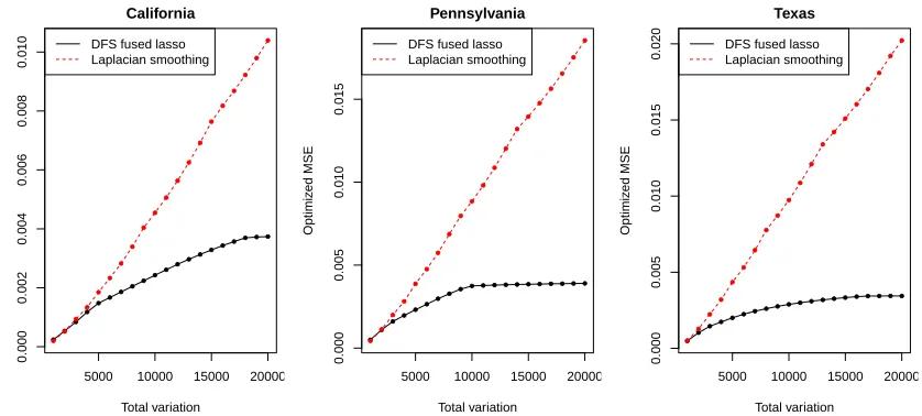
was recorded. Figure 1 displays the optimized MSE for the DFS fused lasso and Laplacian smoothing, as the total variation of the underlying signal varies, for the three road network graphs.
As we can see from the figure, for low values of the underlying total variation, i.e., low signal-to-noise ratio (SNR) levels, Laplacian smoothing and the DFS fused lasso, each tuned to optimality, perform about the same. This is because at low enough SNR levels,
each will be approximating θ0 by something like ¯y1, with ¯y being the sample average of
the data vector y. But as the SNR increases, we see that the DFS fused lasso outpeforms
● ● ● ● ●● ●● ●● ●● ●● ●● ●●●●
5000 10000 15000 20000
0.000 0.002 0.004 0.006 0.008 0.010 California Total variation Optimiz ed MSE ● ● ● ● ● ● ● ● ● ● ● ● ● ● ● ● ● ● ● ●
DFS fused lasso Laplacian smoothing ● ● ●● ●● ●● ●●●●●●●●●●●●
5000 10000 15000 20000
0.000 0.005 0.010 0.015 Pennsylvania Total variation Optimiz ed MSE ● ● ● ● ● ● ● ● ● ● ● ● ● ● ● ● ● ● ● ●
DFS fused lasso Laplacian smoothing
● ●●
●●
●●●●●●●●●●●●●●●
5000 10000 15000 20000
0.000 0.005 0.010 0.015 0.020 Texas Total variation Optimiz ed MSE ● ● ● ● ● ● ● ● ● ● ● ● ● ● ● ● ● ● ● ●
DFS fused lasso Laplacian smoothing
Figure 1: The optimized MSE for the DFS fused lasso and Laplacian smoothing (i.e., MSE achieved
by these methods under optimal tuning) is plotted as a function of the total variation of the underlying signal, for each of the three road network graphs. This has been averaged over 50 draws of data y for each construction of the underlying signal θ0, and 10 repetitions in constructing θ0 itself. For low values of the underlying total variation, i.e., low SNR levels, the two methods perform about the same, but as the SNR increases, the DFS fused lasso outperforms Laplacian smoothing by a considerable margin.
Laplacian smoothing by a considerable amount. This might seem surprising, as Laplacian smoothing uses information from the entire graph, whereas the DFS fused lasso reduces the rich structure of the road network graph in each case to that of an embedded chain.
However, Laplacian smoothing is a linear smoother (meaning that ˆθLap in (29) is a linear
function of the data y), and therefore it comes with certain limitations when estimating
signals of bounded variation (e.g., see the seminal work of Donoho and Johnstone (1998), and the more recent graph-based work of Sadhanala et al. (2016)). In contrast, the DFS fused lasso is a nonlinear estimator, and while it discards some information in the original graph structure, it retains enough of the strong adaptivity properties of the fused lasso over the original graph to statistically dominate a linear estimator like Laplacian smoothing.
Lastly, in terms of computational time, it took an average of 82.67 seconds, 44.02 sec-onds, and 54.49 seconds to compute the 20 DFS fused lasso solutions (i.e., over the 20 tuning parameter values) for the road network graphs from California, Pennsylvania, and
Texas, respectively (the averages are taken over the 50 draws of datay around each signal
θ0, and the 10 repetitions in constructingθ0). By comparison, it took an average of 2748.26
seconds, 1891.97 seconds, and 1487.36 seconds to compute the 20 Laplacian smoothing so-lutions for the same graphs. The computations and timings were performed on a standard laptop computer (with a 2.80GHz Intel Core i7-2640M processor). For the DFS fused lasso,
in each problem instance, we first computed a DFS ordering using the dfs function from
the R package igraph, which is an R wrapper for a C++ implementation of DFS, and
initialized the algorithm at a random node for the root. We then computed the appropriate
is an R wrapper for a C++ implementation of the fast (linear-time) dynamic programming
algorithm in Johnson (2013). For Laplacian smoothing, we used the solve function from
the R package Matrix, which is an R wrapper for a C++ implementation of the sparse
Cholesky-based solver in Davis and Hager (2009). For such large graphs, alternative al-gorithms, such as (preconditioned) conjugate gradient methods, could certainly be more efficient in computing Laplacian smoothing solutions; our reported timings are only meant to indicate that the DFS fused lasso is efficiently computable at problem sizes that are large enough that even a simple linear method like Laplacian smoothing becomes nontrivial.
5.2 2d grid graphs
Next we consider a denoising example on a 2d grid graph of dimension 1000×1000, so
that the number of nodes is n = 1000000 and the number of edges is m = 1998000. We
generated a synthetic piecewise constant signal θ0 ∈R1000×1000 over the 2d grid, shown in
the top left corner of Figure 2, where a color scale (displayed in the accompanying color legend) is used, with red denoting the smallest possible value and yellow the largest possible
value. Data y∈R1000×1000 was generated by adding i.i.d. N(0,1) noise to the components
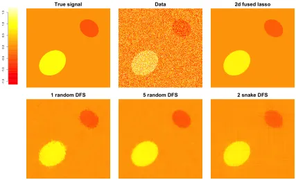
of θ0, displayed in the top middle panel of Figure 2. We then computed the 2d fused lasso
solution, i.e., the fused lasso solution over the full 2d grid2graph, as well as three DFS-based
variations: the DFS fused lasso solution using a random DFS ordering (given by running DFS beginning at a random node), labeled as “1 random DFS” in the figure; the average of DFS fused lasso solutions over 5 random DFS orderings, labeled “5 random DFS” in the figure; and the average of DFS fused lasso solutions over 2 “snake” DFS orderings (one given by collecting and joining all horizontal edges and the other all vertical edges) labeled “2 snake DFS” in the figure. The tuning parameter for each method displayed in the figure was
chosen to minimize the average MSE over 100 draws of the datayfrom the specified model.
Visually, we can see that the full 2d fused lasso solution is the most accurate, however, the 1 random DFS, 5 random DFS, and 2 snake DFS solutions all still clearly capture the structure inherent in the underlying signal. Of the three DFS variations, the 5 random DFS estimator is visually most accurate; the 1 random DFS estimator is comparably “blotchy”, and the 2 snake DFS estimator is comparably “stripey”.
The left panel of 3 shows the optimized MSE for each method, i.e., the minimum of
the average MSE over 100 draws of the datay, when we consider 20 choices for the tuning
parameter. This optimized MSE is plotted as a function of the sample size, which runs
from n = 2500 (a 50×50 grid) to n = 1000000 (a 1000×1000 grid), and in each case
the underlying signal is formed by taking an appropriate (sub)resolution of the image in the top left panel of Figure 2. The 2d fused lasso provides the fastest decrease in MSE
as n grows, followed by the 5 random DFS estimator, then the 1 random DFS estimator,
and the 2 snake DFS estimator. This is not a surprise, since the 2d fused lasso uses the information from the full 2d grid. Indeed, comparing (11) and (19), we recall that the 2d
fused lasso enjoys an MSE rate of tlog2n/nwhen θ0 has 2d total variation t, whereas the
DFS fused lasso has an MSE rate of only (t/n)2/3 in this setting. Whent√n, which is a natural scaling for the underlying total variation in 2d and also the scaling considered in the experimental setup for the figure, these rates are (log2n)n−1/2 for the 2d fused lasso,
and n−1/3 for the DFS fused lasso. The figure uses a log-log plot, so the MSE curves all
appear to have linear trends, and the fitted slopes roughly match these theoretical MSE rates (-0.58 for the 2d fused lasso, and -0.39, -0.40, and -0.36 for the three DFS variations).
The right panel of Figure 3 shows the runtimes for each method (averaged over 100 draws
of the datay), as a function of the sample sizen. The runtime for each method counts the
total time taken to compute solutions across 20 tuning parameter values. The computations and timings were carried out on a standard desktop computer (with a 3.40GHz Intel Core
i7-4770 processor). To compute 2d fused lasso solutions, we used the TVgen function in
the Matlab package proxTV, which is a Matlab wrapper for a C++ implementation of
the proximal stacking technique described in Barbero and Sra (2014). For the DFS fused
lasso, we computed initial DFS orderings using thedfs function from the Matlab package
MathBGL, and then, as before, used the C++ implementation available through glmgento compute the appropriate 1d fused lasso solutions. The figure uses a log-log plot, and hence we can see that all DFS-based estimators are quite a bit more efficient than the 2d fused lasso estimator.
5.3 Tree graphs
We finish with denoising comparisons on tree graphs, for sample sizes varying fromn= 100
ton= 5300. For each sample sizen, a random tree is constructed via a sequential process in
which each node is assigned a number of children between 2 and 10 (uniformly at random).
Given a tree, an underlying signal θ0 ∈ Rn is constructed to be piecewise constant with
total variation 5√n (the piecewise constant construction here is made easy because the
oriented incidence matrix of a tree is invertible). Data y ∈ Rn was generated by adding
i.i.d.N(0,1) noise toθ0. We compared the fused lasso estimator over the full tree, 1 random
DFS and 5 random DFS estimators (using the terminology from the last subsection), and the wavelet smoothing estimator defined in (26). For each estimator, we computed the entire solution path using the path algorithm of Tibshirani and Taylor (2011) implemented
in the R packagegenlasso, and selected the step along the path to minimize the average
MSE over 50 draws of data y around θ0, and 10 repetitions in constructing θ0. (The full
solution path can be computed here because each estimator can be cast as a generalized lasso problem, and because the problem sizes considered here are not enormous.)
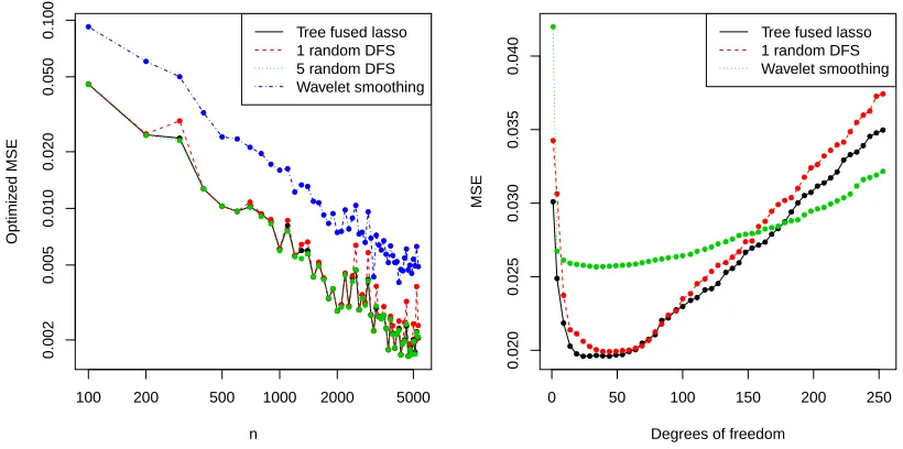
The left panel of Figure 4 plots this optimized MSE as a function of the sample size n.
We see that the fused lasso estimator over the full tree and the 5 random DFS estimator perform more or less equivalently over all sample sizes. The 1 random DFS estimator is slightly worse, and the wavelet smoothing estimator is considerably worse. The right panel shows the the MSE as a function of the effective degrees of freedom of each estimator,
for a particular data instance with n= 5300. We see that both the tree fused lasso and 1
Figure 2: Underlying signal, data, and solutions from the 2d fused lasso and different variations on the DFS fused lasso fit over a 1000×1000grid.
● ● ● ● ● ● ● ● ● ● ● ● ● ● ● ● ● ● ● ●
2e+03 1e+04 5e+04 2e+05 1e+06
0.001 0.002 0.005 0.010 0.020 n Optimiz ed MSE ● ● ● ● ● ● ● ● ● ● ● ● ● ● ● ● ● ●● ● ● ● ● ● ● ● ● ● ● ● ● ● ● ● ●● ● ●● ● ● ● ● ● ● ● ● ● ● ● ● ● ● ● ● ● ● ●● ●
2d fused lasso (slope: −0.58) 1 random DFS (slope: −0.39) 5 random DFS (slope: −0.40) 2 snake DFS (slope: −0.36)
● ● ● ● ● ● ● ● ● ● ● ● ●● ●● ●● ●●
2e+03 1e+04 5e+04 2e+05 1e+06
0.01 0.05 0.50 5.00 50.00 n
Runtime in seconds
● ● ● ● ● ● ● ● ● ● ● ● ●● ●● ● ● ●● ● ● ● ● ● ● ● ● ● ● ● ● ●● ● ●● ●● ● ● ● ● ● ● ● ● ● ● ● ● ● ●● ● ●● ●● ●
2d fused lasso 1 random DFS 5 random DFS 2 snake DFS
Figure 3: Optimized MSE and runtime for the 2d fused lasso and DFS fused lasso estimators over
● ● ● ● ● ● ●● ● ● ● ●● ● ● ● ● ● ● ●● ● ● ● ● ● ● ● ● ● ● ● ●●● ● ● ● ● ● ●● ● ●● ● ● ● ● ● ● ● ●
100 200 500 1000 2000 5000
0.002 0.005 0.010 0.020 0.050 0.100 n Optimiz ed MSE ● ● ● ● ● ● ● ● ● ● ● ● ● ● ● ● ● ● ● ●● ● ● ● ● ● ● ● ● ● ● ● ●● ● ● ● ● ● ● ● ● ● ● ● ● ● ● ● ● ● ● ● ● ● ● ● ● ● ● ● ● ● ● ● ●● ● ● ● ● ● ●● ● ● ● ● ● ● ● ● ● ● ● ●●● ● ● ● ● ● ●● ● ●● ● ●●● ● ● ● ● ● ● ● ● ● ● ● ● ● ● ● ●● ● ●● ● ● ● ●● ● ● ● ● ●● ● ● ● ● ● ● ● ● ● ● ● ● ●● ● ●● ● ● ●● ● ● ● ● ● Tree fused lasso 1 random DFS 5 random DFS Wavelet smoothing ● ● ● ● ● ● ● ● ● ● ● ●● ● ●●● ● ● ●● ● ● ● ●● ●● ● ●● ● ● ●● ● ● ● ●● ●●● ● ●● ● ● ●● ●
0 50 100 150 200 250
0.020
0.025
0.030
0.035
0.040
Degrees of freedom
MSE ● ● ● ● ● ● ●● ● ● ● ● ● ●●● ● ● ●● ●● ●● ●● ● ●● ● ● ●● ●● ● ● ● ● ●● ●● ● ● ● ● ●● ● ● ● ● ● ● ● ● ● ● ● ● ● ● ● ● ●● ● ●● ● ● ● ●● ● ● ●● ● ● ●●● ● ● ● ● ● ●● ● ●● ● ●● ●● ● ●●
Tree fused lasso 1 random DFS Wavelet smoothing
Figure 4: The left panel shows the optimized MSE as a function of the sample size n for the fused
lasso over a tree graph, as well as the 1 random DFS and 5 random DFS estimators, and wavelet smoothing. The right panel shows the MSE as a function of the degrees of freedom of each estimator, for a particular data example withn= 5300.
6. Discussion
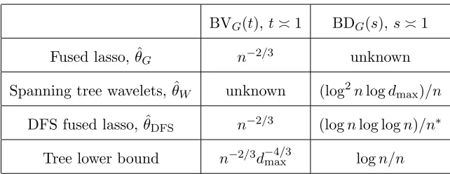
Recently, there has been a significant amount on interest on graph-structured denoising. Much of this work has focused on the construction of graph kernels or wavelet bases. We have proposed and studied a simple method, defined by computing the 1d fused lasso over a particular DFS-induced ordering of the nodes of a general graph. This linear-time algorithm comes with strong theoretical guarantees for signals of bounded variation (achieving optimal MSE rates for trees of bounded degree), as well as guarantees for signals with a bounded number of nonzero differences (achieving nearly optimal rates under a condition on the spacings of jumps along the DFS-induced chain). We summarize our theoretical results in Table 1.
Practically, we have seen that the DFS fused lasso can often represent a useful trade-off between computational efficiency and statistical accuracy, versus competing methods that offer better statistical denoising power but are more computationally expensive, especially for large problems. A simple trick like averaging multiple DFS fused lasso fits, over multiple random DFS-induced chains, often improves statistical accuracy at little increased compu-tational cost. Several extensions along these lines, and other lines, are possible. To study any of them in detail is beyond the scope of this paper. We discuss them briefly below, leaving detailed follow-up to future work.
6.1 Beyond simple averaging
Given multiple DFS fused lasso estimators, ˆθDFS(1) , . . . ,θˆ(DFSK), obtained using multiple
DFS-induced chains computed on the same graphG, there are several possibilities for intelligently
combining these estimators beyond the simple average, denoted (say) ¯θ(DFSK) = (1/K)PK
k=1θˆ
BVG(t), t1 BDG(s),s1
Fused lasso, ˆθG n−2/3 unknown
Spanning tree wavelets, ˆθW unknown (log2nlogdmax)/n
DFS fused lasso, ˆθDFS n−2/3 (lognlog logn)/n∗
Tree lower bound n−2/3d−max4/3 logn/n
Table 1: A summary of the theoretical results derived in this paper. All rates are on the mean
squared error (MSE) scale (Ekθˆ−θ0k2
n for an estimator θˆ), and for simplicity, are presented under
a constant scaling fort, s, the radii in theBVG(t),BDG(s)classes, respectively. The superscript “∗”
in theBDG(s)rate for the DFS fused lasso is used to emphasize that this rate only holds under the
assumption thatWn n. Also, we write dmax to denote the max degree of the graph in question.
To better preserve edges in the combined estimator, we could run a simple nonlinear filter— for example, a median filter, over ˆθ(1)DFS, . . . ,θˆ(DFSK) (meaning that the combined estimator is defined by taking medians over local neighborhoods of all of the individual estimators). A more sophisticated approach would be to compute the DFS fused lasso estimators
sequen-tially, using the (k−1)st estimator to modify the response in some way in the 1d fused
lasso problem that defines the kth DFS fused lasso estimator. We are intentionally vague
here with the specifics, because such a modification could be implemented in various ways; for example, it could be useful to borrow ideas from the boosting literature, which would have us treat each DFS fused lasso estimator as a weak learner.
6.2 Distributed algorithm
For large graphs, we should be able to both compute a DFS ordering over G, and solve
the DFS fused lasso problem in (18), in a distributed fashion. There are many algorithms for distributed DFS, offering a variety of communication and time complexities; see, e.g., Tsin (2002) for a survey. Distributed algorithms for the 1d fused lasso are not as common, though we can appeal to the now well-studied framework for distributed optimization via the alternating direction method of multipliers (ADMM) from Boyd et al. (2011). Different formulations for the auxiliary variables present us with different options for communication
costs. We have found that, for a formulation that requires O(1)-length messages to be
communicated between processors, the algorithm typically converges in a reasonably small number of iterations.
6.3 Theory for piecewise constant signals
The bounded differences class BDG(s) in (5) is defined in terms of the cut metric k∇Gθk0
of a parameterθ, which recall, counts the number of nonzero differences occurring inθover
edges in the graphG. The cut metric measures a notion of strong sparsity (compared to the
weaker notion measured by the total variation metric) in a signalθ, over edge differences;
the cut metric k∇Gθk0 can actually be quite large for a parameter θ that is piecewise
constant overG, with a small number of pieces—these are groups of connected nodes that
are assigned the same constant value inθ. Over the 2d grid graph, e.g., one can easily define
a parameterθthat has only (say) two constant pieces but on the order of√nnonzero edge
differences. Therefore, for such a “simple” configuration of the parameterθ, the cut metric
k∇Gθk0 is deceivingly large.
To formally define a metric that measures the number of constant pieces in a parameter
θ, with respect to a graphG= (V, E), we introduce a bit of notation. Denote byZ(θ)⊆E
the subset of edges over whichθexhibits differences of zero, i.e.,Z(θ) ={e∈E:θe+ =θe−}.
Also write (∇G)Z(θ) for the submatrix of the edge incidence matrix ∇G with rows indexed
by Z(θ). We consider a metric defined by
ρG(θ) = nullity (∇G)Z(θ)
,
where nullity(·) denotes the dimension of the null space of its argument. An equivalent
definition is
ρG(θ) = the number of connected components in (V, E\Z(θ)).
We may now define thepiecewise constant class, with respect toG, and a parameters >0,
PCG(s) ={θ∈Rn:ρG(θ)≤s}.
It is not hard to to see that BVG(s)⊆PCG(s) (assuming only that G is connected), but
for certain graph topologies, the latter class PCG(s) will be much larger. Indeed, to repeat
what we conveyed above, for the 2d grid one can naturally define a parameterθ such that
θ∈BDG(
√
n) andθ∈PCG(2).
We conjecture that the fused lasso estimator over Gcan achieve a fast MSE rate when
the meanθ0 in (1) exhibits a small number of constant pieces, i.e., θ0∈PCG(s), provided
that these pieces are of roughly equal size.
6.4 Weighted graphs
The key result in Lemma 1 can be extended to the setting of a weighted graphG= (V, E, w),
withwe≥0 denoting the edge weight associated to an edge e∈E.
Lemma 9 Let G = (V, E, w) be a connected weighted graph, where recall we write V =
{1, . . . , n}, and we assume all edge weights are nonnegative. Consider running DFS on G,
and denote by τ :{1, . . . , n} → {1, . . . , n} the induced permutation, so that if v1, . . . , vn are
the nodes in the order that they are traversed by DFS, then
τ(i) =vi, for all i= 1, . . . , n.
Denote wmin= mine∈Ewe, the minimum edge weight present in the graph, and define
˜
wτ(i),τ(i+1) =
(
we if e={τ(i), τ(i+ 1)} ∈E,
wmin otherwise,
It holds that
n−1
X
i=1
˜
wτ(i),τ(i+1)
θτ(i+1)−θτ(i) ≤2
X
e∈E
we|θe+ −θe−|, for all θ∈Rn, (31)
as well as
n−1
X
i=1
˜
wτ(i),τ(i+1)1
θτ(i+1) 6=θτ(i) ≤2
X
e∈E
we1{θe+ 6=θe−}, for all θ∈Rn. (32)
Remark 10 As with Lemma 1, Lemma 9 has also essentially appeared in the literature, in a form for binary signals and the roughness metric being the quadratic form in the graph Laplacian, see Cesa-Bianchi et al. (2013). The main idea behind this result and Lemma 9 is the same, and the latter follows from the former with only minor modifications.
For simplicity, when edges in the DFS chain do not appear in the original graph, we have defined their corresponding weights to be the minimum of the weights in the original graph. Instead, we could have taken the approach in Cesa-Bianchi et al. (2013), and defined the weight for such an edge in the DFS chain to be the minimum of weights from original edges in its backtracking path.
The bounds in (31), (32) are the analogies of (15), (16) but for a weighted graph G;
indeed we see that we can still embed a DFS chain into G, but this chain itself comes
with edge weights, as in (30). These new edge weights in the chain do not cause any computational issues; the 1d fused lasso problem with arbitrary penalty weights can still be
solved in O(n) time using the taut string algorithm in Barbero and Sra (2014). Thus, in
principle, all of the results in this paper should carry over in some form to weighted graphs.
6.5 Robustness to signal perturbation
Here we briefly explore some robustness properties of the DFS fused lasso estimator, under
perbutations of the mean parameter θ0 in (1) with respect to a small number of nodes.
This is based on the approach taken by Cesa-Bianchi et al. (2013) to study robustness in
their online graph-structured classification setting. Let G = (V, E, w) a weighted graph,
and write k∇Gθk1 for the weighted total variation of a signal θ, i.e.,
k∇Gθk1 =
X
e∈E
we|θe+−θe−|.
Denote byθδ a perturbed version ofθ, where any number of entries are given by adding an
amount δ >0 to the corresponding entries of θ. (More general forms of perturbations can
also be investigated but slightly complicate the discussion that follows, so for simplicity, we will limit ourselves to considering this simple model for perturbations.) Denote by
I(θ, θδ) =
n
i∈ {1, . . . , n} : θi 6=θδi