Interleaved Text/Image Deep Mining on a Large-Scale Radiology Database for Automated Image Interpretation

(1)

Journal of Machine Learning Research 17 (2016) 1-31 Submitted 5/15; Revised 4/16; Published 6/16

Interleaved Text/Image Deep Mining on a Large-Scale

Radiology Database for Automated Image Interpretation

Hoo-Chang Shin [email protected]

Le Lu [email protected]

Lauren Kim [email protected]

Ari Seff [email protected]

Jianhua Yao [email protected]

Ronald M. Summers [email protected]

Imaging Biomarkers and Computer-Aided Diagnosis Laboratory Radiology and Imaging Sciences

National Institutes of Health Clinical Center Bethesda, MD 20892-1182, USA

Editor:Benjamin M. Marlin, C. David Page, and Suchi Saria

Abstract

Despite tremendous progress in computer vision, there has not been an attempt to apply machine learning on very large-scale medical image databases. We present an interleaved text/image deep learning system to extract and mine the semantic interactions of radiology images and reports from a national research hospital’s Picture Archiving and Communica-tion System. With natural language processing, we mine a collecCommunica-tion of∼216K represen-tative two-dimensional images selected by clinicians for diagnostic reference and match the images with their descriptions in an automated manner. We then employ a weakly super-vised approach using all of our available data to build models for generating approximate interpretations of patient images. Finally, we demonstrate a more strictly supervised ap-proach to detect the presence and absence of a number of frequent disease types, providing more specific interpretations of patient scans. A relatively small amount of data is used for this part, due to the challenge in gathering quality labels from large raw text data. Our work shows the feasibility of large-scale learning and prediction in electronic patient records available in most modern clinical institutions. It also demonstrates the trade-offs to consider in designing machine learning systems for analyzing large medical data. Keywords: Deep learning, Convolutional Neural Networks, Topic Models, Natural Lan-guage Processing, Medical Imaging

1. Introduction

(2)

Russakovsky et al. (2015). In the medical domain, however, there are no similar large-scale labeled image data sets available. On the other hand, large collections of radiology images and reports are stored in many modern hospitals’ Picture Archiving and Communication Systems (PACS). The invaluable semantic diagnostic knowledge inhabiting the mapping between hundreds of thousands of clinician-created high-quality text reports and linked image volumes remains largely unexplored. One of our primary goals is to extract and associate radiology images with clinically semantic labels via interleaved text/image data mining and deep learning on a large-scale PACS database (∼780K imaging examinations). To the best of our knowledge, this is the first reported work performing automated mining and prediction on a hospital PACS database at a very large scale.

The Radiology reports are text documents describing patient history, symptoms, image observations and impressions written by board-certified radiologists. However, the reports do not contain specific image labels to be trained by a machine learning algorithm. Build-ing the ImageNet database (Deng et al., 2009) was mainly a manual process: harvestBuild-ing images returned from Google image search engine according to the WordNet (Miller, 1995) ontology hierarchy and pruning falsely tagged images using crowd-sourcing such as Amazon Mechanical Turk (AMT). This does not meet our data collection and labeling needs due to the demanding difficulties of medical annotation tasks and the need for data privacy. Thus, we first propose to mine categorical semantic labels using a non-parametric topic modeling method—latent Dirichlet Allocation (LDA) by Blei et al. (2003)—to provide a semantic interpretation of a patient image in three levels. While this provides a first-level interpre-tation of a patient image, labeling based on categorization can be nonspecific. To alleviate the issue of non-specificity, we further mine specific disease words in the reports mentioning the images. Feed-forward CNNs were then used to train and predict the presence/absence of the specific disease categories.

Our work has been inspired by the works of Deng et al. (2009); Russakovsky et al. (2015) building very large-scale image databases and the works establishing semantic con-nections of texts and images by Kulkarni et al. (2013). Please note that there has not yet been much comparable development on large-scale medical imaging interpretation. Kulka-rni et al. (2013) have spearheaded the efforts of leaKulka-rning the semantic connections between image contents and the sentences describing them, such as image captions. Detecting ob-jects of interest, attributes and prepositions and applying contextual regularization with a conditional random field (CRF) is a feasible approach as shown by Kulkarni et al. (2013), and many useful tools for image annotation using it are available in computer vision.

In this work, both deep feed-forward CNNs of Krizhevsky et al. (2012); Simonyan and Zisserman (2015) and word-embedding networks of Mikolov et al. (2013a,b) are used to model image and text. Also, the CNN parameters pre-trained on ImageNet are used to initialize CNNs for medical image analysis. We show the benefit of this transfer learning

and domain adaptation in Section 4.2. The fact that deep learning requires no

(3)

Text/Image Mining on a Large-Scale Radiology Database

1.1 Related Work

The ImageCLEF medical image annotation tasks of 2005-2007 by Deselaers and Ney (2008)

have 9,000 training and 1,000 test images, converted to 32×32 pixel thumbnails with

57 labels. Local image descriptors and intensity histograms are used as a bag-of-features approach for this scene-recognition-like problem. However, the data set is limited to radio-graphs (for example, chest and bone x-rays), and it is difficult to detect any disease from

32×32 size images. Unsupervised LDA-based matching from lung disease words (for

ex-ample, fibrosis, emphysema) to two-dimensional image blocks from axial CT chest scans is studied by Carrivick et al. (2005) where data were collected from a relatively small number (24) of patients. The works of Barnard et al. (2003); Blei and Jordan (2003) using gener-ative models of combining words and images under a very limited word/image vocabulary has also motivated this study.

Socher et al. (2013); Frome et al. (2013) first map words into vector space using recurrent neural networks and then project images into the label-associated word-vector embeddings

by minimizing theL2 (Socher et al., 2013) or hinge rank losses (Frome et al., 2013) between

the visual and label manifolds. The language model is trained on the texts of Wikipedia and tested on label-associated images from the CIFAR (Krizhevsky and Hinton, 2009; Socher et al., 2013) and ImageNet data sets (Deng et al., 2009; Frome et al., 2013). Image-to-language correspondence was learned from the ImageNet data set and reasonably high quality image description data sets (Pascal1K (Rashtchian et al., 2010), Flickr8K (Hodosh et al., 2013), Flickr30K (Young et al., 2014), MS-COCO Lin et al. (2014)) by Karpathy et al. (2014); Vinyals et al. (2015); Donahue et al. (2015); Xu et al. (2015); Mao et al. (2015), where such caption data sets are not available in the medical domain.

The tasks of mining and labeling images from a data set of blog posts with user photos and related texts and retrieving them with query words were demonstrated in Kim et al. (2015b,a, 2014). Similarly, a noisy image-text data set consisting of product photos (such as bags, clothing and shoes) and their associated text description (Berg et al., 2010) was used to demonstrate image retrieval with text queries and image description generation. Nonetheless, they all require pre-trained models either from the large ImageNet data set or a large text data set (for example, word representations trained on Wikipedia or Reuters news data sets (Turian et al., 2010)). Still there exists no such large data set of images and texts in the medical domain.

(4)

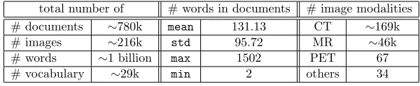
total number of # words in documents # image modalities

# documents ∼780k mean 131.13 CT ∼169k

# images ∼216k std 95.72 MR ∼46k

# words ∼1 billion max 1502 PET 67

# vocabulary ∼29k min 2 others 34

Table 1: Some statistics of the data set. “Others” include computed radiography, and

ultrasound.

2. Data

To gain the most comprehensive interpretation of diagnostic semantics, we use all available radiology reports of around 780,000 imaging examinations, stored in the PACS of National Institutes of Health Clinical Center since the year 2000. Around 216,000 two-dimensional representative image slices referred by doctors are studied here, instead of using all three-dimensional image volumes. Within three-three-dimensional patient scans, most of the imaging information represented are normal anatomy, therefore they are often not the focus of the radiology reports. The two-dimensional “key images” referenced by radiologists manually during radiology report writing provide a visual reference to pathologies or other notable findings (Figure 1). Therefore, the two-dimensional key images are more correlated with the diagnostic semantics in the reports than the whole three-dimensional scans, but not all reports have referenced key images (215,786 images from about 61,845 unique patients). Table 1 provides some statistics of the extracted database, and Table 2 shows examples of the most frequently occurring words in the radiology reports collected. Leveraging our deep learning models exploited in this paper will make it possible to automatically select key images from three-dimensional patient scans to avoid mis-referencing.

Finding and extracting key images from radiology reports is done by natural language processing (NLP), that is, finding a sentence mentioning a referenced image. For example, “There may be mild fat stranding of the right parapharyngeal soft tissues (series 1001, image

32)” is listed in Figure 1. The NLP steps are sentence tokenization, word/number matching

and stemming, and rule-based information extraction (for example, translating “image

1013-78” to “images 1013-101013-78”). A total of ∼187K images are retrieved and matched this way,

whereas the rest of ∼28K key images were extracted according to their reference accession

numbers in PACS. The image-text matching is accurate as we use exact annotations from the sentences in reports in retrieving the images, however, it is possible we missed some image-text pairs due to limitations in our NLP pipelines. We do not evaluate the recall-rate of our method in this study, but it can be considered as a future work. The software package of Bird et al. (2009) is used for the basic NLP pipelines.

3. Document Topic Learning with Latent Dirichlet Allocation

It is difficult to annotate the∼216K images and the sentences referring to them. Unlike the

(5)

0001 REPORT : REASON FOR EXAM (Entered by ordering clinician into CRIS): hx of head and neck cancer. needs scan CT of the nasopharynx.

HISTORY: Head and neck cancer.

TECHNIQUE: Contiguous 2.5 mm axial images of the nasopharynx were performed without IV contrast. COMPARISON: xx/xx/xxxx.

FINDINGS: No soft tissue masses are seen within the soft tissues of the neck. The parotid and submandibular glands are predominantly fatty-replaced. Soft tissues of the Naso, oropharynx are unremarkable. There may be mild fat stranding of the right parapharyngeal soft tissues (series 1001, image 32). No abnormal masses are seen at that site. No bulky lymphadenopathy is seen. There is a fusiform aneurysm of the basilar artery as previously described. It appears to the mildly increased in size and currently measures 2.0 cm in transverse dimensions and previously measured 1.8 cm. It measured 1.5 cm in transverse dimensions on xx/xx/xxxx. Atherosclerotic calcifications are also seen within the carotid arteries bilaterally. There is near-complete opacification of the maxillary sinuses bilaterally. This has increased predominantly within the left maxillary sinus and mildly within the right maxillary sinus. The ethmoidal air cells are clear. Sphenoidal and frontal sinuses are clear. Degenerative changes of the cervical spine are noted.

IMPRESSIONS: 1. No soft tissue masses however, mild right parapharyngeal fat stranding is seen it may be postoperative or post radiation in nature. 2. Basilar artery aneurysm that has gradually increased in size when compared to prior examinations. 3. Atherosclerotic disease of the coronary arteries bilaterally..

0001 Report: CHEST, ABDOMEN, PELVIS CT: Multidetector helical (5 mm, quad) images following, and abdomen images prior to vascular contrast infusion (45 s delay, 2 cc/s, 130 cc Isovue) obtained without apparent complication. History: renal cell pt on Medarex protocol here for end of course evaluation.

CHEST: Multiple right, and at least one left lung masses minimally-moderately increasing since xx/xx/xxxx, compatible with metastases despite moderate decrease in at least one right mid-lung mass (e.g. series 4 image 30). Minimal pretracheal and subcarinal adenopathy increasing. Spine osteophytes. Enlargement thyroid on right side, and thyroid heterogeneity unchanged, possibly due to goiter. No evidence of pleural or pericardial effusion, axilla or left hilum adenopathy.

ABDOMEN, PELVIS: Few right and left liver foci, left periaortic and left adrenal fossa, and right sacrum mass and lytic lesion (series 3 image 88-95) increasing minimally, compatible with metastases. Scattered lumbar vertebra and bilateral ilium foci (e.g. series 3 image 55, 60, 80, 84-7, 96) foci possibly due to bone metastases. Uterine fundus focus (series 3 image 95) increasing in density since xx/xx/xxxx, possibly due to fibroid, metastasis. No evidence of splenomegaly, hydronephrosis, gallbladder calcification, or bulky mesenteric adenopathy.

Figure 1: Two examples of radiology reports and the referenced “key images” (providing a visual reference to pathologies or other notable findings).

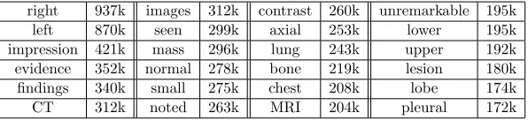
right 937k images 312k contrast 260k unremarkable 195k

left 870k seen 299k axial 253k lower 195k

impression 421k mass 296k lung 243k upper 192k evidence 352k normal 278k bone 219k lesion 180k findings 340k small 275k chest 208k lobe 174k

CT 312k noted 263k MRI 204k pleural 172k

Table 2: Examples of the most frequently occurring words in the radiology report docu-ments.

several organs usually with pathologies. There is a high amount of intrinsic ambiguity in defining and assigning a semantic label set to images, even for experienced clinicians. We therefore propose to mine image categorization labels using the non-parametric

(6)

hypothesis is that the large collection of radiology reports statistically defines the categories meaningful for topic-mining and visual correspondence learning for these topics.

Latent Dirichlet Allocation (LDA) was originally proposed by Blei et al. (2003) to find latent topics for a collection of text documents such as newspaper articles. There are some other popular methods for document topic modeling, such as Probabilistic Latent Semantic Analysis (pLSA) by Hofmann (1999) and Non-negative Matrix Factorization (NMF) by Lee and Seung (1999). In a study done by Stevens et al. (2012) LDA showed the most favorable results overall in human evaluations of the generated topics compared to other popular methods. Furthermore, pLSA can be regarded as a special case of LDA (Girolami

and Kab´an, 2003) and NMF as a semi-equivalent model of pLSA (Gaussier and Goutte,

2005; Ding et al., 2006).

LDA offers a hierarchy of extracted topics and the number of topics can be chosen by

evaluating each model’s perplexity score (Equation 1), which is a common way to measure

how well a probabilistic model generalizes by evaluating the log-likelihood of the model on a

held-out validation set. For an unseen document setDval, the perplexity score is defined as

in Equation 1, whereM is the number of documents in the validation set, wd the words in

the unseen document d,Ndthe number of words in document d, withΦthe topic matrix,

and α the hyper-parameter for topic distribution of the documents.

perplexity(Dval) = exp

(

−

PM

d=1logp(wd|Φ, α)

PM

d=1Nd

)

(1)

A lower perplexity score generally implies a better fit of the model for a given document set (Blei et al., 2003).

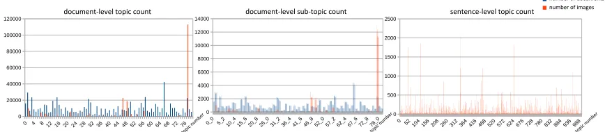
Based on the perplexity score evaluated on 80% of the total documents used for training and 20% used for validation, the number of topics chosen is 80 for the document-level model using perplexity scores for model selection (Figure 2). Although the document distribution in the topic space is approximately balanced, the distribution of image counts for the topics is more unbalanced (Figure 3). Specifically, topic #77 (non-primary metastasis spreading

across a variety of body parts) contains nearly half of the ∼216K key images. To address

this data bias, sub-topics are obtained for each of the first document-level topics, resulting in 800 topics, where the number of the sub-topics is also chosen based on the average perplexity scores evaluated on each document-level topic. Lastly, to compare the method of using the whole report with using only the sentence directly describing the key images for latent topic mining, sentence-level LDA topics are obtained based on three sentences only: the sentence mentioning the key-image (Figure 1) and its adjacent sentences as proximal context. The perplexity scores keep decreasing with an increasing number of topics; we choose the topic count to be 1000 as the rate of the perplexity score decrease is very small beyond that point (Figure 2).

We observe that LDA-generated image categorization labels are valid, demonstrating good semantic coherence among clinician observers. Some examples of document-level topics with their corresponding images and topic key words are shown in Figure 4. All reports and sentences referring to the images have associated topics, and images are sampled from

the sentences belonging to the multi-level topics. The lists of key words and sampled

(7)

10 20 30 40 50 60 70 80 90 100 840 860 880 900 920 940 960 980 1000 1020

perplexity scores for document-level topic model

perplexity

number of topics

pe rp le xi ty 0 50 100 150 200 250 300 350 400 450 500

perplexity scores for sentence-level topic model

perplexity

number of topics

pe

rp

le

xi

ty

10 20 30 40 50 60 70 80 90 100

840 860 880 900 920 940 960 980 1000 1020

perplexity

number of topics

pe rp le xi ty 0 50 100 150 200 250 300 350 400 450 500

perplexity

number of topics

pe rp le xi ty number#of#topics# number#of#topics# pe rp le xi ty #

Figure 2: Perplexity scores for document-/sentence- level topic models. Number of topics with low perplexity score is selected as the optimal (80 for document-level, 1000 for sentence-level). 0 20000 40000 60000 80000 100000 120000

document-level topic count

#documents #images 0 2000 4000 6000 8000 10000 12000 14000

document-level 2nd hierarchy topic count

#documents #images 0 20000 40000 60000 80000 100000 120000

#documents #images 0 500 1000 1500 2000 2500

sentence-level topic count

#images 0 20000 40000 60000 80000 100000 120000

#documents #images

10 20 30 40 50 60 70 80 90 100

840 860 880 900 920 940 960 980 1000 1020

perplexity #topics pe rp le xi ty 0 50 100 150 200 250 300 350 400 450 500

perplexity #topics pe rp le xi ty

10 20 30 40 50 60 70 80 90 100 840 860 880 900 920 940 960 980 1000 1020

perplexity #topics pe rp le xi ty 0 50 100 150 200 250 300 350 400 450 500

perplexity #topics pe rp le xi ty number#of#documents# number#of#images#

documentXlevel#topic#count# documentXlevel#subXtopic#count# sentenceXlevel#topic#count#

Figure 3: Distribution of documents and images for document-level topic, document-level sub-topic, and sentence-level topic. Sixth sub-topic (second-level topic) of (first-level) document topic 41 is noted as 40 5.

There are 73 low-level concepts, for example, pathology examination of certain body regions and organs: topic #47 - sinus diseases; #2 - lesions of solid abdominal organs, primarily kidney; #10 - pulmonary diseases; #13 - brain MRI; #19 - renal diseases on mixed imaging modalities; #36 brain tumors. There are 7 mid to highlevel concepts, such as: topic #77 -non-primary metastasis spreading across a variety of body parts; topic #79 - cases with high diagnosis uncertainty or equivocation; #72 - indeterminate lesions; #74 - instrumentation artifacts limiting interpretation. Low-level topic images tend to be visually more coherent than the higher-level topic images.

(8)

Topic&04:&

axial,contrast,mri,sagiWal,post,flair,enha ncement,blood,dynamic,brain,relaLve,v olume,this,precontrast,from,tesla,fse,di ffusion,gradient,resecLon,comparisons, maps,philips,progression,some,suscepL bility,perfusion,stable,achieva,techniqu e,echo,weighted,1.5,evidence,mass,# findings,hemorrhage,enhanced,impressi on,frontal,signal,coronal,dL,tumor,t1X ffe,hydrocephalus,magnevist,reformaLo ns,bolus,lesion#

Topic&17:&

breast,performed,suspicious,breasts,see n,impression,mass,screening,mammogr am,dated,annual,cancer,mri,benign,bila teral,was,biXrads,mammograms,# NegaLve,dense,history,calciﬁcaLons,im ages,views,studies,quadrant,mammogra phy,volume,organ,aspect,suggested,cat egory,mastectomy,before,Lssue,enhanc ement,microcalciﬁcaLons,heterogeneo usly,prior,family,examinaLon,recomme nd,malignancy,high,suggest,outer,mass es,developing,clip,paLent#

Topic&31:&

spine,cord,cervical,thoracic,spinal,level, canal,lumbar,sagiWal,vertebral,neural,di sc,signal,mri,body,technique,levels,ﬁndi ngs,foramina,mild,disk,nerve,within,sm all,marrow,central,bodies,normal,impre ssion,enhancing,conus,syrinx,this,narro wing,lesions,roots,contrast,throughout, bone,degeneraLve,foramen,protrusion, mulLple,l5Xs1,also,abnormal,c5Xc6,# posterior,changes,heights#

Topic&78:&

bone,lesion,hip,knee,femoral,lyLc,femu r,proximal,head,scleroLc,joint,shoulder, hips,evidence,pelvis,distal,lesions,ﬁndin gs,humeral,lateral,fracture,medial,hum erus,focal,impression,bony,prosthesis,hi story,iliac,pain,bilateral,blasLc,avn,acet abulum,seen,marrow,sclerosis,view,bot h,osteolyLc,corLcal,heads,area,cortex,e ﬀusion,replacement,Lbial,involving,con sistent,views#

#

Figure 4: Examples of LDA generated document-level topics with corresponding images and key words. Topic #4 is MRI of brain tumor; topic #17: breast imaging; topic #31: degenerative spine disc disease; and topic #78: bone metastases. These are verified by a radiologist.

‘chest port catheter’, ‘chest imaging with disease or pathology’, and ‘degenerative disease in bone’.

We also obtained LDA topics on the reports having associated images only, resulting in 20 topics according to perplexity score. However, these did not add any more meaningful semantics in addition to the already obtained topics in three levels, so that we do not include the topics. For more details and the image-topic associations, refer to Figures 4, 5, and the supplementary material. Even though LDA labels are computed with text information only, we next investigate the plausibility of mapping images to the topic labels of different levels via deep CNN models.

4. Image to Document Topic Mapping with Deep Convolutional Neural Networks

(9)

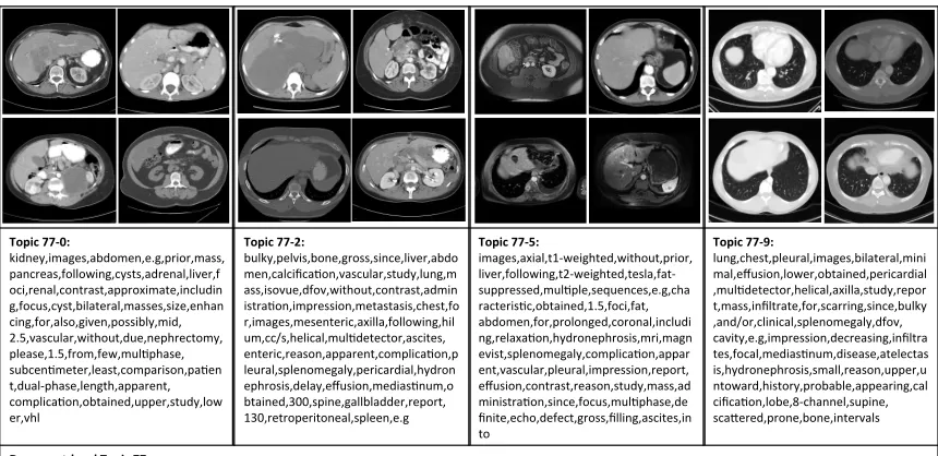
Topic&77.0:&

kidney,images,abdomen,e.g,prior,mass, pancreas,following,cysts,adrenal,liver,f oci,renal,contrast,approximate,includin g,focus,cyst,bilateral,masses,size,enhan cing,for,also,given,possibly,mid, 2.5,vascular,without,due,nephrectomy, please,1.5,from,few,mulLphase,# subcenLmeter,least,comparison,paLen t,dualXphase,length,apparent,# complicaLon,obtained,upper,study,low er,vhl#

Topic&77.2:&

bulky,pelvis,bone,gross,since,liver,abdo men,calciﬁcaLon,vascular,study,lung,m ass,isovue,dfov,without,contrast,admin istraLon,impression,metastasis,chest,fo r,images,mesenteric,axilla,following,hil um,cc/s,helical,mulLdetector,ascites,# enteric,reason,apparent,complicaLon,p leural,splenomegaly,pericardial,hydron ephrosis,delay,eﬀusion,mediasLnum,o btained,300,spine,gallbladder,report, 130,retroperitoneal,spleen,e.g#

Topic&77.5:&

images,axial,t1Xweighted,without,prior,# liver,following,t2Xweighted,tesla,fatX suppressed,mulLple,sequences,e.g,cha racterisLc,obtained,1.5,foci,fat,# abdomen,for,prolonged,coronal,includi ng,relaxaLon,hydronephrosis,mri,magn evist,splenomegaly,complicaLon,appar ent,vascular,pleural,impression,report, effusion,contrast,reason,study,mass,ad ministraLon,since,focus,mulLphase,de finite,echo,defect,gross,filling,ascites,in to#

Topic&77.9:&

lung,chest,pleural,images,bilateral,mini mal,effusion,lower,obtained,pericardial ,mulLdetector,helical,axilla,study,repor t,mass,infiltrate,for,scarring,since,bulky ,and/or,clinical,splenomegaly,dfov,# cavity,e.g,impression,decreasing,infiltra tes,focal,mediasLnum,disease,atelectas is,hydronephrosis,small,reason,upper,u ntoward,history,probable,appearing,cal cificaLon,lobe,8Xchannel,supine,# scaWered,prone,bone,intervals#

Document.level&Topic&77:&

compaLble,adenopathy,series,unchanged,image,evidence,images,e.g,pelvis,lung,since,abdomen,vascular,minimal,foci,bulky,mass,calciﬁcaLon,bone,chest,contrast,liver,e ﬀusion,pleural,obtained,gross,following,without,splenomegaly,axilla,hydronephrosis,metastasis,bilateral,pericardial,increasing,helical,mulLdetector,apparent,complicaL on,hilum,due,spine,gallbladder,administraLon,mesenteric,fat,dfov,cc/s,appearing,delay#

Figure 5: Examples of some sub-topics of document-level topic #77, with corresponding images and topic key-words. The key-words and the images for the document-level topic (#77) indicates metastatic disease. The key-words for topic #77 are:

[abdomen,pelvis,chest,contrast,performed,oral,was,present,masses,stable,intravenous,adenopathy,

liver,retroperitoneal,comparison,administration,scans,130,small,parenchymal,mediastinal,dated, after,which,evidence,were,pulmonary,made,adrenal,prior,pelvic,without,cysts,spleen,mass,disease, multiple,isovue-300,obtained,areas,consistent,nodules,changes,pleural,lesions,following,abdominal, that,hilar,axillary].

and 717 for the sentence-level mapping. Systematic diagrams showing how each level of semantic topics are learned, assigned to images, and trained to map from images to topics are shown in Figure 6.

4.1 Implementation

(10)

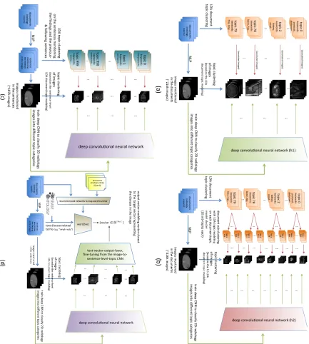
(a) $ (b)$ (c)$ (d)$ deep$convoluBonal$neural$network$ deep$convoluBonal$neural$network$ documents* (medical*ar0cles* (OpenI))* documents* (medical*ar0cles* (OpenI))* documents* (medical*ar0cles* (OpenI))* recurrent*neural*networks*to*map*word*to*vector* word2vec* text:vector:output:layer,* fine:tuning*from*the*image:to: sentence:level:topic*CNN* documents* (medical*ar0cles* (OpenI))* documents* (medical*ar0cles* (OpenI))* documents* (medical*ar0cles* (OpenI))* recurrent*neural*networks*to*map*word*to*vector* word2vec* text:vector:output:layer,* fine:tuning*from*the*image:to: sentence:level:topic*CNN* documents* (medical*ar0cles* (OpenI))* documents* (medical*ar0cles* (OpenI))* documents* (medical*ar0cles* (OpenI))* recurrent*neural*networks*to*map*word*to*vector* word2vec* text:vector:output:layer,* fine:tuning*from*the*image:to: sentence:level:topic*CNN* documents* (medical*ar0cles* (OpenI))* documents* (medical*ar0cles* (OpenI))* documents* (medical*ar0cles* (OpenI))* recurrent*neural*networks*to*map*word*to*vector* word2vec* text:vector:output:layer,* fine:tuning*from*the*image:to: sentence:level:topic*CNN* documents* (medical*ar0cles* (OpenI))* documents* (medical*ar0cles* (OpenI))*documents* (medical*ar0cles* (OpenI))* recurrent*neural*networks*to*map*word*to*vector* word2vec* text:vector:output:layer,* fine:tuning*from*the*image:to: sentence:level:topic*CNN* ou tp ut* ve cto r*m od elin g*v ec to r*c lo se st* * to *th e*tar ge t*v ec to r*r ep re se n0 ng ** th e*d ise as e*in *th e*im ag e*

Figure 6: Systematic diagrams for training CNNs to learn to classify images into (a) document-level topics (b) document-level sub-topics, (c) sentence-level topics. A systematic diagram for image-to-word model (in Section 5.3) is shown in (d).

(11)

(a)

(

(b)

(

(c)

(

Test(accuracy(vs.(itera9ons( Test(accuracy(vs.(itera9ons( Test(accuracy(vs.(itera9ons(

Te

st(

ac

cu

rac

y(

AlexNet(with(random(ini9aliza9on( AlexNet(with(ImageNet(ini9aliza9on(

VGGNet(with(ImageNet(ini9aliza9on( VGGNet(with(random(ini9aliza9on(

AlexNet(with(random(ini9aliza9on( AlexNet(with(ImageNet(ini9aliza9on( AlexNet(with(ini9aliza9on(from(model((a)(

AlexNet(with(random(ini9aliza9on( AlexNet(with(ImageNet(ini9aliza9on( AlexNet(with(ini9aliza9on(from(model((a)( AlexNet(with(ini9aliza9on(from(model((b)(

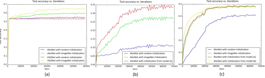
Figure 7: Traces of classification accuracies during training, showing the benefits of us-ing ImageNet data set as pre-trainus-ing for this task with medical images and improvements of fine-tuning from CNN neural networks of similar tasks (for ex-ample, from document-level (h1) CNN model to document-level sub-topic (h2) CNN model). (a) Image-to-document-level-topic (h1) classification, (b) image-to-document-level-sub-topic (h2) classification, and (c) image-to-sentence-level-topic (h3) classification.

sub-topics, and sentence-level respectively. The networks for first-level semantic labels are fine-tuned from the pre-trained ImageNet models, where the networks for the lower-level semantic labels are fine-tuned from the models of the higher-level semantic labels.

4.2 Transfer Learning and Domain Adaptation

We find that transfer learning from the ImageNet pre-trained CNN parameters on natural images to our medical image modalities (mostly CT, MRI) significantly helps the image classification performance. Additionally, transfer learning from a CNN trained for a more related task (for example, from CNN trained on the image-to-document-level-topic models to train CNN for the image-to-document-level-sub-topic model) is found to be more effective than from a CNN trained for a less related task (for example, from CNN trained on ImageNet

to train CNN for image-to-document-level-sub-topic model). Examples of classification

accuracy traces during training using CNNs from random initialization, transfer learning from CNN trained on ImageNet and transfer learning from higher level image-to-topic model to lower level image-to-topic models are shown in Figure 7. Similar findings that deep CNN features can be generalized across different image modalities have been reported by Gupta et al. (2014, 2013) but are empirically verified with only much smaller data sets than ours. Our key image data set is about one-fifth the size of ImageNet (Russakovsky et al., 2015) and is the largest annotated medical image data set to date.

From Figure 7 we can see that: (1) CNN testing accuracy quickly increases from ∼0%

(12)

more closely related task CNN model is even better than fine-tuning from less related task

model (alexnet tp80 h2 start tp80h1> alexnet tp80 h2 start imagenet).

With these findings, we train our CNN models with transfer-learning by default for the remaining parts of our study. All the CNN layers except the newly modified ones are initialized with the weights of a previously trained related model and trained with a new task with a low learning rate of 0.001. The modified layers with a new number of classes are initialized randomly, and their learning rates are set with a higher learning rate of 0.01.

All the key images are re-sampled to a spatial resolution of 256×256 pixels. Then we follow

the approach of Simonyan and Zisserman (2015) to crop the input images from 256×256

to 227×227 for training.

4.3 Classification Results and Discussion

We would expect that the level of difficulties for learning and classifying the images into the LDA-induced topics will be different for each semantic level. Low-level semantic classes can have key images of axial/sagittal/coronal slices with position variations and across MRI/CT modalities. Mid- to high-level concepts all demonstrate much larger within-class variations in their visual appearance since they are diseases occurring within different organs and are only coherent at high-level semantics. Table 3 provides the top-1 and top-5 testing in classification accuracies for each level of topic models using AlexNet (Krizhevsky et al., 2012), and VGG-16&19 Simonyan and Zisserman (2015) based deep CNN models.

All top-5 accuracy scores are significantly higher than top-1 values, for example,

increas-ing from 0.658 to 0.946 using VGG-19, or 0.607 to 0.929 via AlexNet in document-level. This

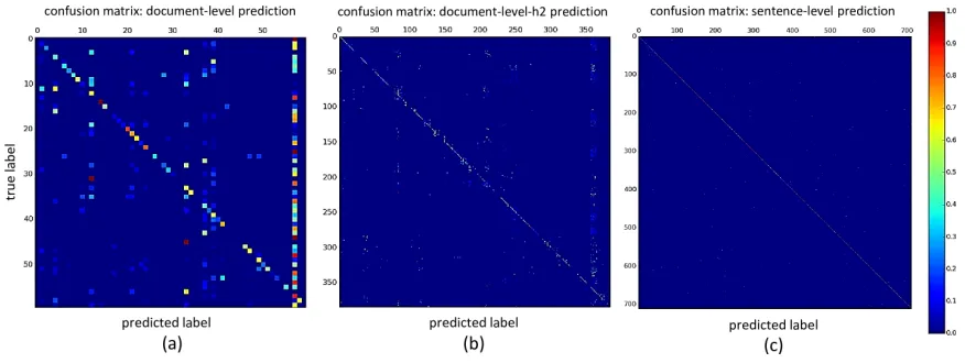
indicates that the classification errors or fusions are not uniformly distributed among other false classes. Latent “blocky subspace of classes” may exist in our discovered label space, where several topic classes form a tightly correlated subgroup. The confusion matrices in Figure 8 verify this finding.

It is shown that the deeper models (VGG-16&19) perform consistently better than the shallower 8-layer model (AlexNet) in classification accuracy, especially for document-level sub-topics. While the images of some topic categories and some body parts are easily distinguishable as shown in Figure 4, the visual differences in abdominal parts are rather subtle as in Figure 5. Distinguishing the subtleties and high-level concept categories in the images could benefit from a more complex model so that the model can handle these subtleties.

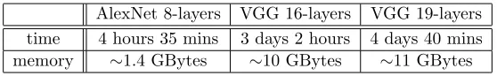
It is also noticeable that VGG-16&19 models require significantly more computational resource and time to train than the shallower model. Table 4 shows the memory consump-tion and time required to train the CNN models for the image-to-sentence-level-topic model with up to 70,000 iterations using the NVidia Tesla K40 GPU. However, comparing VGG-16 and VGG-19, three additional convolutional layers seem to have contributed to raise the top-5 accuracies by a small amount (∼2%), which is coherent with the results reported by Simonyan and Zisserman (2015) for object recognition task on the ImageNet data set.

Compared with the ImageNet 2014 results, top-1 error rates are moderately higher (34%

versus 30%) and top-5 test errors (6%−8%) are comparable. In summary, our quantitative

(13)

AlexNet 8-layers VGG 16-layers VGG 19-layers top-1 top-5 top-1 top-5 top-1 top-5 document-level 0.61 0.93 0.66 0.93 0.66 0.95 document-level-h2 0.33 0.56 0.54 0.70 0.54 0.70 sentence-level 0.48 0.56 0.50 0.56 0.50 0.58

Table 3: Top-1, top-5 test classification accuracies for image to document-level topics, document-level sub-topics (document-level-h2) and sentence-level topics, using AlexNet (Krizhevsky et al., 2012), and VGG-16&19 (Simonyan and Zisserman, 2015) deep CNN models.

Figure 8: Confusion matrices of (a) document-level topic, (b) document-level sub-topic

(document-level-h2), and (c) sentence- level classification Simonyan and Zisserman (2015) ((b) and (c) can be viewed best in electronic version of this document).

show good image learnability by deep CNN models which shed light on the feasibility of automatically parsing very large-scale radiology image databases.

5. Generating Image-to-Text Description

(14)

AlexNet 8-layers VGG 16-layers VGG 19-layers

time 4 hours 35 mins 3 days 2 hours 4 days 40 mins memory ∼1.4 GBytes ∼10 GBytes ∼11 GBytes

Table 4: Training times for the CNN models used to reach 70,000 iterations, and their memory consumption, using Caffe framework (Jia et al., 2014) on NVidia Tesla K40 GPU.

−0.4 −0.2 0.0 0.2 0.4 0.6

− 0.4 − 0.2 0.0 0.2 0.4 Comp.1 Comp .2 mass lobulated huge heterogeneous lesion enhancing cystic heterogenously measuring inhomogeneouslyheterogenously spine lumbar lumbosacral cervical vertebrae spinal vertebra vertebral thoracic pancreas pancreatic spleen

gallbladderhepaticportal

splenic axial coronal demonstrates t1 mr saggital transverse sagital t2 weighted t1wi mri fracture comminuted dislocation fractures fractured deformity clinical clinically evaluation radiological poor documented calcification calcifications appearances eccentric thickening hyperdense

heartcardiacsystolicbeat atrial pulmonale regurgitation findings finding pathology evidence suspected_tentative pathological colon sigmoid ileum colonic cecum ileo rectum caecum small

largeappearanceseen_well

confined around

surrounding

Figure 9: Example words embedded in the vector space using word-to-vector modeling (https://code.google.com/p/word2vec/) visualized on a two-dimensional space, showing (clinical) words with similar meanings are located nearby in the vector space (colors are used to highlight these in visualization).

5.1 Word-to-Vector Modeling and Removing Word-Level Ambiguity

In radiology reports, there exist many recurring word morphisms in text identification, for example, [mr, mri, t1-/t2-weighted] (natural language expressions for imaging modalities of magnetic resonance imaging (MRI)), [cyst, cystic, cysts], [tumor, tumour, tumors, metas-tasis, metastatic], etc. We train the word-to-vector embedding model of Mikolov et al. (2013c,b,a) to address this word-level labeling space ambiguity while also transforming the words to vectors. A total of 1.2 billion words from our radiology reports as well as from

biomedical research articles obtained from OpenI (ope: http://openi.nlm.nih.gov) are

used. Words with similar meaning are mapped or projected to closer locations in the

(15)

~1.2%billion%words%with%OpenI%

#

“cyst”#

cysts#######0.799191# ###hydaLd######0.734686# ####cysLc######0.701855# unilocular######0.654273# ###tailgut######0.639764# nonparasiLc######0.621647# epidermoid######0.604492# ####lipoma######0.588372# ####cheesy######0.586947# mulLloculated######0.584199# ####pearly######0.583126# mulLlocular######0.582670# ####lesion######0.579009# ######tgdc######0.578533# mulLseptate######0.575851# # ~1%billion%words%reports%only% #

#“cyst”#

#cysts####0.768382# ##septated####0.586067# #####polyp####0.583761# ####simple####0.534717# #septaLon####0.500951# parapelvic####0.500877# incidental####0.500760# #####small####0.487211# ####cysLc####0.477632# ######pole####0.471933# mulLseptated####0.469851# ####polyps####0.464380# #exophyLc####0.459088# hyperdense####0.457558# ####mucous####0.448427# ~1.2%billion%words%with%OpenI% #

“heart”#

cardiac#####0.672690# respiratory######0.644453# ######beat######0.642630# ##pressure######0.558879# ####murmur######0.551323# ##systolic######0.548490# pericardial######0.538957# dobutamine######0.537429# intracardiac######0.533799# #####great######0.532735# ######rate######0.531352# #####beats######0.524729# ####atrial######0.524052# tachycardia######0.521093# ####minute######0.520249# # ~1%billion%words%reports%only% #

#“heart”#

#lungs#######0.526600# ###mediasLnum######0.517008# #consolidaLng######0.486605# ############pa######0.449816# #########chest######0.433362# ###infiltrates######0.428404# #hyperinflated######0.413326# ##cardiomegaly######0.410785# ###hyperlucent######0.400836# ########pectus######0.396142# #########great######0.395712# #######ectaLc######0.394560# #######shiVed######0.389205# ###########ray######0.389091# ####infiltrate######0.387224# ~1.2%billion%words%with%OpenI% #

“brain”#

hemisphere######0.684149# hemispheric######0.668626# cerebellum######0.663902# #####whole######0.661564# ###regions######0.647632# #######mri######0.646674# structural######0.638171# neuroanatomical######0.636563# ###crinion######0.626951# ########in######0.626707# parasaggital######0.618392# illustraLon######0.610440# ##striatal######0.609282# ####brains######0.607442# behavioral######0.606803# # ~1%billion%words%reports%only% #

#“brain”#

t1######0.615066# #######mri######0.595027# ##sagiWal######0.580841# #####ﬂair######0.565445# ########t2######0.555053# #####axial######0.554040# ######spgr######0.520954# ##weighted######0.502047# #technique######0.487768# astrocytoma######0.480527# #######gbm######0.476956# ##gradient######0.476593# oligodendroglioma######0.465892# postcontrast######0.463686# ########3d######0.458123# ~1.2%billion%words%with%OpenI% #

“liver”#

hepaLc#####0.764163# ####spleen######0.683242# #cirrhoLc######0.664428# #cirrhosis######0.664262# #######hcc######0.656473# ####portal######0.610437# hepatocellular######0.603930# parenchyma######0.597169# ###splenic######0.579957# hepatomegaly######0.573687# #####tumor######0.571135# ###abdomen######0.559092# hepatectomy######0.556156# ######bclc######0.546798# subcapsular######0.542745# # ~1%billion%words%reports%only% #

#“liver”#

spleen######0.759884# ###gallbladder######0.648075# ##hepatomegaly######0.642022# ####gallstones######0.611837# ######pancreas######0.608356# #####gallstone######0.606063# #####steatosis######0.601081# ##########dome######0.594812# ########portal######0.570008# #######ascites######0.551869# hepatosplenomegaly######0.540501# #######hepaLc######0.537453# #####cirrhosis######0.530389# #########faWy######0.522134# #######kidneys######0.515252#

Figure 10: Word-to-vector models trained on a collection of biomedical research articles (from OpenI ope) and radiology reports, and radiology reports only. Search words (with quotes) and their closest words in vector-space cosine similarity (higher the better) are listed in a descending order.

A skip-gram model of Mikolov et al. (2013a,b) is employed with the mapping vector

dimension of R256×1 per word, trained using the hierarchical softmax cost function, the

sliding-window size of 10 and frequent words sub-sampled in the frequency of 0.01. It is found that combining an additional, more diverse set of related documents such as OpenI biomedical research articles, is helpful for the model to learn a better vector representation while keeping all the hyper-parameters the same. Similar findings on unsupervised feature learning models, that robust features can be learned from a slightly noisy and diverse set of input, were reported by Vincent et al. (2010, 2008); Shin et al. (2013). Some examples of query words and their corresponding closest words with respect to cosine similarity for the word-to-vector models (Mikolov et al., 2013c), which are trained on radiology reports only

(total of∼1 billion words) and with additional OpenI articles (total of 1.2 billion words),

(16)

#words/sentence mean median std max min

reports-wide 11.70 9 8.97 1014 1

image references 23.22 19 16.99 221 4

image references, no stopwords no digits 13.46 11 9.94 143 2 image references, disease terms only 5.17 4 2.52 25 1

Table 5: Some statistics about number of words per sentence—across the radiology reports (reports-wide), across the sentences identifying the key images and its two adjacent ones (image references) and these not counting stop-words and digits as well as counting disease related words only.

5.2 Image-to-Description Relation Mining and Matching

The sentence referring to a key image and its adjacent sentences may contain a variety of words, but we are mostly interested in the disease-related terms which are highly correlated to diagnostic semantics. To obtain only the disease-related terms, we exploit the human disease terms and their synonyms from the Disease-Ontology (DO; Schriml et al. (2012)), a collection of 8,707 unique disease-related terms. While the sentences referring to an image and their adjacent sentences have 50.08 words on average, the number of disease-related

terms in the three consecutive sentences is 5.17 on average with a standard deviation of 2.5.

Therefore, we chose to use bi-grams for the image descriptions, to achieve a good trade-off between the medium level complexity without neglecting too many text-image pairs. Some statistics about the number of words in the documents are shown in Table 5.

Bi-gram disease terms are extracted so that we can train a deep CNN model in Section

5.3 to predict the vector-/word- level image representation of R256×2. If multiple bi-grams

can be extracted per image from the sentence referring the image and the two adjacent ones, the image is trained as many times as the number of different bi-grams with different

target vectors (R256×2). If a disease term cannot form a bi-gram, then the term is ignored,

where the process is illustrated in Figure 11. This is a challengingweakly annotated learning

problem using referring sentences for labels. The bi-grams of DO disease-related terms in

the vector representation ofR256×2 are somewhat analogous to the work of Kulkarni et al.

(2013) detecting multiple objects of interest and describing their spatial configurations in the image caption. A deep regression CNN model is employed here, to map an image to a continuous output word-vector space from an image. The resulting bi-gram vector can be matched against a reference disease-related vocabulary in the word-vector space using cosine similarity.

5.3 Image-to-Words Deep CNN Regression

(17)

Figure 11: Illustration of how word sequences are learned for an image. Bi-grams are

selected from the image’s reference sentences containing disease-related terms from the disease ontology (DO; Schriml et al. (2012)). Each bi-gram is

con-verted to a vector of Z ∈ _R256×2 _{to learn from an image. Image input}

vec-tors as {X ∈ R256×256} are learned through a CNN by minimizing the

cross-entropy loss between the target vector and output vector. The words “nodes” and “hepatis” in the second line are DO terms but are ignored since they

can not form a bi-gram. The DO logo is reproduced with permission from

http://disease-ontology.org.

softmax cost in Section 4 with the cross-entropy cost function for the last output layer of VGG-19 CNN model (Simonyan and Zisserman, 2015):

E=−1

n

N

X

n=1

[g(z)nˆg(¯zn) + (1−g(zn)) log(1−g(ˆzn))], (2)

whereznor ˆznis any uni-element of the target word vectorsZnor optimized output vectors

ˆ

Zn, g(x) is the sigmoid function (g(x) = 1/(1 +e−x)), and n is the number of samples in

(18)

We adopt the CNN model of Simonyan and Zisserman (2015) for the image-to-text representation since it works consistently better than the other relatively simpler model of Krizhevsky et al. (2012) in our image-to-topic mapping tasks. We fine-tune the parameters of the CNNs for predicting the topic-level labels in Section 4 with the modified cost function, to model the image-to-text representation instead of classifying images into categories. The newly modified output layer has 512 nodes for bi-grams as 256 nodes for each word in a bi-gram.

5.4 Key-Word Generation from Images and Discussion

For any key image in testing, first, we predict its topics at three levels (document-level, document-level sub-topics, sentence-level) using the three deep CNN models of Simonyan and Zisserman (2015) in Section 4. Based on each word’s probability of appearing in the LDA document topic, the fifty key-words with highest probability are mapped into the

word-to-vector space of multivariate variables in R256×1 (Section 5.1). Then, the image is

mapped to aR256×2 output vector using the bi-gram CNN model in Section 5.3. Lastly, we

match each of the 50 topic key-word vectors of R256×1 against the first and second half of

the R256×2 output vector using cosine similarity. The closest key-words at three levels of

topics (with the highest cosine similarity against either of the bi-gram words) are kept per image.

The rate of predicted disease-related words matching the actual words in the report sentences of test set (recall-at-K, K=1 (R@1 score)) is 0.56. Two examples of key-word generation are shown in Figure 12, with three key-words from three categorization levels per image. We only report R@1 score on disease-related words compared to the previous works of Karpathy et al. (2014); Frome et al. (2013), where they report from R@1 up to R@20 on the entire image caption words (for example, R@1=0.16 on Flickr30K data set by Karpathy et al. (2014)). As we use NLP to parse and extract image-describing sentences from the radiology reports, our ground-truth image-to-text associations are much noisier than the caption data set used by Frome et al. (2013); Karpathy et al. (2014). Also for that reason, our generated image-to-text associations are not as exact as the generated descriptions by Frome et al. (2013); Karpathy et al. (2014).

5.4.1 Discussion

Generating key-words for images by CNN regression shows good feasibility for automated interpretation of patient images. The generated key-words describe what to expect from the given image, although sometimes unrelated words can be generated too. Finding and understanding the relations between the generated words will be the next step to explore, for example via more thorough text mining using sophisticated NLP parsing as by Li et al. (2011) and combining them with the specific frequent disease prediction in the next section.

6. Predicting Presence or Absence of Frequent Disease Types

(19)

Input image Output text Original text

Figure 12: Examples of text key-word generation results, and average cosine distances be-tween the generated words from the disease-related words in the original texts. The word “diameter” appears in the original radiology report of the first image, but not much can be derived by the word only. The rate of predicted disease-related words matching the actual words in the report sentences (recall-at-K, K=1 (R@1 score)) on test set is 0.56.

would be to automatically diagnose disease from a patient scan. In order to achieve the goal of automated disease detection, we add an additional pipeline of mining disease words rather than disease-related words using radiology semantics and predicting these in an image using CNNs with softmax cost-function.

6.1 Mining Presence/Absence of Frequent Disease Terms

The disease names in Disease Ontology (DO) contain not only disease terms but also

non-disease terms describing a non-disease. Some examples of disease names in DO containing

non-disease terms are “occlusion of gallbladder” (DOID: 9714), “acute diarrhea” (DOID: 0050140), “strawberry gallbladder” (DOID: 10254), and “exocrine pancreatic insufficiency” (DOID: 13316). Nonetheless, it is rare that “occlusion of gallbladder” or “exocrine pancre-atic insufficiency” is described in radiology reports exactly that way, making it difficult to mine specific disease terms with presence or absence.

The Unified Medical Language System (UMLS) of Lindberg et al. (1993); Humphreys et al. (1998) integrates and distributes key terminology, classification and coding stan-dards, and associated resources to promote the creation of more effective and inter-operable biomedical information systems and services, including electronic health records. It is a compendium of many controlled vocabularies in the biomedical sciences, created in 1986 and maintained by the National Library of Medicine.

(20)

collected from over 100 incorporated controlled vocabularies and classification systems. The Metathesaurus is organized by concept, where each concept has specific attributes defining its meaning and is linked to the corresponding concept names. The Metathesaurus has 133 semantic types that provide a consistent categorization of all concepts represented in it. Among the 133 semantic types we chose to focus on “T033: finding” and “T047: disease or syndrome”, as they seemed most relevant to be disease specific. Examples of some other semantic types we do not focus on this study are: “T017: anatomical structure”, “T074: medical device”, and “T184: sign or symptom”.

RadLex (Langlotz, 2006) is a unified language to organize and retrieve radiology imaging reports and medical records. While the Metathesaurus has a vast resource of biomedical concepts, we also use RadLex to confine our disease-term-mining more specifically to radi-ology related terms. The mined words are one-word terms appearing in the “T033: finding” and “T047: disease or syndrome” of the UMLS Metathesaurus appearing also in RadLex (RadLex is not a subset of Metathesaurus).

We are not only interested in disease terms associated with an image, but also whether the disease mentioned is present or absent. After detecting semantic terms of “T033: find-ing” and “T047: disease or syndrome”, we use the assertion/negation detection algorithm of Chapman et al. (2001, 2013) to detect presence and absence of disease terms. The algorithm of Chapman et al. (2001, 2013) locates trigger terms which can indicate a clinical condition as negated or possible and determines which text falls within the scope of the trigger terms. The number of occurrences “T033: finding” and “T047: disease or syndrome” detected as assertion or negations in radiology reports are shown in Figure 13.

While the assertion/negation detection of “T047: disease or syndrome” seemed specific enough, the detection of “T033: finding” was not. For example, it seemed difficult to derive any specific disease information from 43,219 occurrences of possible “unchanged” and 422 occurrences of negated “unchanged”. Some other similar examples are: 10,236 occurrences of possible “finding” and 1,129 occurrences of negated “finding”; 3,781 occurrences of pos-sible “t2” (an MRI image modality) and 661 occurrences of negated “t2”. We therefore decided to focus on “T047: disease or syndrome” terms only, and further ignored the terms which occurred less than 10 times in the radiology reports. The total number of “T047: disease or syndrome” terms for detecting their presence are 59, and the total number of the terms for detecting their absence are 18.

6.2 Predicting Disease in Images using CNN

Similarly to the object detection task in the ImageNet challenge, we match and detect disease terms found in the sentences of radiology reports referring to an image using a CNN and softmax cost function.

In addition to assigning disease terms to images, we also assign negated disease terms as the absence of the diseases in the images. The total number of labels is 77 (59 present, 18 absent). If more than one disease term is mentioned for an image, we simply assign the terms multiple times for an image. Some statistics on the number of assertion/negation occurrences per image are shown in Table 6.

(21)

Text/Image Mining on a Large-Scale Radiology Database abscess alkaptonuriaanemia aneurysm appendicitisarthritis arthropathy atherosclerosisbronchiectasis bronchiolitisbronchitis cirrhosiscolitis cyst decubitusdisease emphysemaenteritis enterocolitisesophagitis fasciitis gallstoneganglion goiter granulomatosisgynecomastia hydrocele hydronephrosishypertension infection intussusceptionischemia lymphedemalymphocele mycetomamyositis nephrocalcinosisosteitis osteochondromatosisosteomyelitis osteophyte osteoporosispancreatitis pneumonia pneumonitis pneumoperitoneumpneumothorax prolapse prostatitis pyelonephritissarcoidosis sinusitis spondylosissyndrome synovitis telangiectasiatenosynovitis varix volvulus adenopathyascites bulge bulging collapse diagnosis embolismfever findinglesion lymphadenopathymargin mass opacitypatch perforating perforationplaque related resonanceretraction sensitivityshunt sign stresst1 t2 thickened thickening unchangedunrelated worsening

disease or syndrome

finding

1 2 3 4

frequency ter m abscess alkaptonuriaanemia aneurysm appendicitisarthritis arthropathy atherosclerosisbronchiectasis bronchiolitisbronchitis cirrhosiscolitis cyst decubitusdisease emphysemaenteritis enterocolitisesophagitis fasciitis gallstoneganglion goiter granulomatosisgynecomastia hydrocele hydronephrosishypertension infection intussusceptionischemia lymphedemalymphocele mycetomamyositis nephrocalcinosisosteitis osteochondromatosisosteomyelitis osteophyte osteoporosispancreatitis pneumonia pneumonitis pneumoperitoneumpneumothorax prolapse prostatitis pyelonephritissarcoidosis sinusitis spondylosissyndrome synovitis telangiectasiatenosynovitis varix volvulus adenopathyascites diagnosisfinding lesion lymphadenopathymargin mass opacitypatch relatedt1 t2 thickening unchanged

disease or syndrome

finding

1 2 3 4

frequency

ter

m

(a)$ (b)$

Figure 13: Number of occurrences (frequencies) of semantic terms “T033: finding” and “T047: disease or syndrome” in UMLS Metathesaurus and also appearing in RadLex, detected as (a) assertion and (b) negation in the radiology reports.

Frequencies are shown in log10 scale.

# images per image mean/std # assertions per image # negations per image total matching 18291 # assertions mean 1.05 1/image 16133 1/image 1581 total not matching 197495 # negations mean 1.05 2/image 613 2/image 84

with assertions 16827 # assertions std 0.23 3/image 81 3/image 0 with negations 1665 # negations std 0.22 4/image 0 4/image 0

Table 6: Some statistics of images-to-disease presence/absence label matching.

we fine-tune from the image to sentence-level-topic (h3) model in Section 4, as the image-to-sentence-level-topic seems to be most closely related to the image-to-disease-specific-terms

model. Similarly to Section 4, 85% of image-label pairs are used for training, 5% for

validation, and 10% for testing.

6.3 Prediction Result and Discussion

(22)

previous image-to-topic mapping and key-word generation (Section 5.4) to generate the final output for comprehensive image interpretation. Some examples of test cases where top-1 probability output matches the originally assigned disease labels are shown in Figure 14. It is noticeable that specific disease words are detected with high probability when there is one disease word per image, but with relatively lower top-1 probability for one disease word and other words within the top-5 probabilities (Figure 14 (b)—“ ... infection abscess”).

We also observe that automatic label assignment to images can sometimes be challeng-ing. In Figure 14 (d) “cyst” is assigned as the correct label based on the original statement “... possibly due to cyst ...”, but it would be unclear whether cyst will be present in the image (and the cyst is not visibly apparent). It applies similarly to Figure 14 (e) where the presence of “osteophyte” is not clear from the referring sentence but is assigned as the cor-rect label (and osteophyte is not visibly apparent on the image). In Figure 14 (f) “no cyst” is labeled and predicted correctly, but it is not obvious what to derive from this prediction that indicates an absence of a disease versus a presence.

Some examples of test cases where top-1 probability does not match the originally assigned labels are shown in Figure 15. Four ((a),(c),(e),(f)) of the six examples, however, contain the originally assigned label in the top-5 probability predictions, which is coherent with the relatively high (88%) top-5 prediction accuracy.

Here again, Figure 15 (a) is automatically labeled as “cyst”, but the cyst is not clearly visible on the image where the original statement “... too small to definitely characterize cyst ...” supports this. The example of Figure 15 (b) shows a failed case of assertion/negation algorithm, where “cyst” is detected as negated based on the statement “... small cyst”.

Nonetheless, true label (“cyst”) is detected as its top-1 probability. For Figure 15 (c)

“cyst” is predicted where the true label assigned was “abscess”; however cyst and abscess are sometimes visibly similar. Similarly to Figure 14 (d), it is unclear whether we should expect to find emphysema in the image from the statement such as “ ... possibly due to emphysema” (and emphysema is not visibly present). Therefore, it would be challenging to correctly interpret such statement for label assignment. Figure 15 (e) shows a disease which can be bronchiectasis, but it is also unclear from the image. However, bronchiectasis is predicted with the second highest probability. Bronchiectasis is visible in Figure 15 (f), and it was predicted with second highest probability too.

6.3.1 Discussion

(23)

Input image Generated

key-words originating effusion upper avg distance 0.14 Disease detection cyst: 0.999 no cyst: 2.24e-05 disease: 1.54e-05 gallstone: 5.32e-07 hydronephrosis: 3.48e-07

label: cyst 2 multiple clip artifacts indicative of previous surgery in the

left abdominal wall and left retroperitoneum about the kidney 3 in the upper abdomen non enhancing well defined foci of

high signal intensity on t2 weighted images consistent with cysts one about a centimeter at the left renal splenic interface series 501 image 19 the other less than 5 mm in the periphery

of the right kidney series 501 image 12 4 multiple gallstones

Original text susceptibility findings tibialis avg distance 0.20 abscess: 0.663 infection: 0.103 osteochondromatosis: 0.037 synovitis: 0.032 label: abscess cyst: 0.026

… for example series 701 image 12 and series 401 image 27 with findings suggesting minimally enhancing rim laterally for

example series 1101 image 21 may … the findings suggest a fluid collection with … the location suggests possibility of a

synovial collection synovial thickening as the appearance is

nonspecific correlation with clinical findings is recommended regarding the possibility of an infection abscess

basal fasciitis findings avg distance 0.31 myositis: 0.996 tenosynovitis: 0.002 label: myositis lymphedema: 1.30e-05 fasciitis: 0.002

no myositis: 2.84e-06

images were obtained of both thighs including stir scans

findings include 1 areas of slight increase in signal intensity in

some muscles on the stir scan more apparent on the left than the right for example series 4 image 13 the left hamstrings and vastus medialis consistent with myositis 2 no evidence of

gross fatty infiltration of the muscles

anterior effusion renal avg distance 0.34 cyst: 0.709

no gallstone: 0.050

label: cyst

syndrome: 0.020 lymphocele: 0.120

pyelonephritis: 0.016

adrenal glands 1.2 mm lower right kidney focus e.g series 3 image 63 possibly due to cyst no evidence of pleural effusion

splenomegaly hydronephrosis calcification in gallbladder or kidneys or definite adrenal mass or calcification

subclavian effusion hairy avg distance 0.20 osteophyte: 0.472 gynecomastia: 0.098 label: osteophyte

no hydronephrosis: 0.034 disease: 0.207

pneumothorax: 0.028

history lymphoma restaging chest subcentimeter right apex lung cavity series 921780 image 11 unchanged since xx/xx/ xxxx spine osteophytes no evidence of pleural or pericardial

effusion bulky axilla mediastinum or hilum adenopathy or

lung mass or infiltrate

subclavian effusion

upper

avg distance 0.36

no cyst: 0.488

no hydronephrosis: 0.048

label: no cyst

spondylosis: 0.003 cyst: 0.425

aneurysm: 0.003

the left kidney is essentially unchanged the right kidney however shows two new approximately 2 cm masses series 2 image 69 and series 2 image 74 these are not obviously cysts and given the patient s diagnosis lymphoma involving right kidney is suggested the liver shows several metallic sutures

along the right lobe (a) (b) (c) (f) (d) (e)

(24)

Input image Generated key-words pelvic nodules punctate avg distance 0.40 Disease detection abscess: 0.489 disease: 0.295 cyst: 0.078 aneurysm: 0.051 pneumoperitoneum: 0.023 label: cyst

4 evidence of splenectomy with postoperative changes including clips 5 subcentimeter low attenuation liver focus too

small to definitively characterize cyst series 2 image 66 6 no evidence of developing noncalcified pulmonary nodule renal

mass Original text developme-nt pelvic luxation avg distance 0.27 cyst: 0.995 cirrhosis: 0.001 ischemia: 0.001

no hydronephrosis: 0.001

label: no cyst

gallstone: 0.001

2.9 cm right adrenal mass left adrenal atrophy 2 no evidence of renal lesion save for a 5 mm focus of bright signal intensity at the cortical surface of the upper pole of the left kidney on the t2 weighted scan image 12 series 5 consistent with small

cyst concomitant from findings avg distance 0.32 label: abscess

no cyst: 3.81e-06 abscess: 5.25e-06

no pneumothorax: 7.06e-06

findings the uterus and adnexae are within normal limits

again seen is a small right perirectal abscess and fistula extending to the right perineum with slight decrease size of a component of this fistulous tract at the level of the perineum

that previously measured approximately 1.6 cm

node effusion upper avg distance 0.31 disease: 0.973 label: emphysema

no cyst: 0.001 arthritis: 0.005 osteophyte: 0.005

chest minimal left supraclavicular fossa adenopathy or small lymph node e.g series 2 image 7 probably unchanged since xx/xx/xxxx poorly defined bilateral upper lung radiolucencies

unchanged possibly due to emphysema spine degenerative change bronchopu-lmonary effusion one avg distance 0.20 cyst: 0.441 label: disease disease: 0.044 aneurysm: 0.068 infection: 0.075

there is a small right pericardial effusion that is grossly stable there is increased airspace disease with air bronchograms within the posterior medial aspect of the right upper lung series 4 image 26 this has increased compared to the prior study and may represent infectious etiology or increasing

scarring multifocal upper effusion avg distance 0.57 disease: 0.700 label: bronchiectasis

no cyst: 0.001 infection: 0.002

cyst: 0.007

there remains right upper lobe bronchiectasis and residual mild nodular airspace disease series 2 image 19 anterior right

upper lobe lung nodule again noted series 2 image 23 as well

as additional middle lobe lingular and bilateral lower lobe bronchiectasis and nodular air space disease no pleural or

pericardial effusion

disease: 4.60e-05

no gallstone: 0.013

bronchiectasis: 0.138 bronchiectasis: 0.287 (b) (c) (e) (f) cyst: 0.999 (a) (d)

Figure 15: Some examples of final outputs for automated image interpretation where top-1 probability does not match the originally assigned label. One of the top-5 probabilities match the originally assigned labels in the examples of images (a), (c), (d), and (f). None of the top-5 probabilities match the originally assigned

labels in the examples of image (b) and (d). However, label assignment of

(25)

it than modeling and detecting an image with a more specific term as “cyst” (similarly to “finding” or “unchanged”).

It is a compromise between whether to go for big data and loose labels or to go for smaller data and more accurate labels. The key-word generation from the rather loose labeling scheme enables us to use most of the available 216K images. While the generated key-words can help understand the contents of the image, sometimes they are not specific and can also be irrelevant. More specific mining and assignment of specific disease labels to images could provide more accurate and precise disease prediction; however, only about 10% of the total images are made available by this scheme. Another alternative is to obtain annotation by radiologists to be even more specific, but the amount of data available will be even smaller due to the time and cost limitations.

Consequently, utilizing bigger data will enable us to make a more generalizable model, but labeling will become more challenging as the amount of data gets bigger and becomes more heterogeneous. The compromise between the amount of data and the quality of labels seems to be a recurring dilemma in the majority of automated mining in big data appli-cations. More advanced NLP techniques and comprehensive analysis of hospital discharge summaries, progress notes, and patient histories might address the need to obtain more specific information relating to an image even when the original image descriptions are not very specific.

7. Conclusion

It has been unclear how to extend the significant success in image classification using deep convolutional neural networks from computer vision to medical imaging. What are the clinically relevant image labels to be defined, how to annotate the huge amount of medical images required by deep learning models, and to what extent and scale the deep CNN architecture is generalizable to medical image analysis are open questions.

In this paper, we present an interleaved text/image deep mining system to extract the semantic interactions of radiology reports and diagnostic key images at a very large, un-precedented scale in the medical domain. Images are classified into hierarchies of topics according to their associated documents, and a neural language model is learned to assign disease terms to predict the image interpretation. However, by generating the “attributes” of patient images, the generated descriptions are not disease-specific, whereas one of the primary goals for medical image analysis is to automatically diagnose diseases. In order to address this issue, we mine and match frequent disease types using disease ontology and semantics, and demonstrate prediction of the presence/absence of disease with probability outputs. Yet, only about 10% of the entire data set could be used for this study due to the challenge of more precisely matching the disease words with semantics. This raises inter-esting questions regarding the trade-offs in designing a machine learning system analyzing large medical data.