Rate Optimal Denoising of Simultaneously Sparse and Low
Rank Matrices
Dan Yang [email protected]
Department of Statistics and Biostatistics Rutgers University
Piscataway, NJ 08854, USA
Zongming Ma [email protected]
Andreas Buja [email protected]
Department of Statistics University of Pennsylvania Philadelphia, PA 19104, USA
Editor:Hui Zou
Abstract
We study minimax rates for denoising simultaneously sparse and low rank matrices in high dimensions. We show that an iterative thresholding algorithm achieves (near) optimal rates adaptively under mild conditions for a large class of loss functions. Numerical experi-ments on synthetic datasets also demonstrate the competitive performance of the proposed method.
Keywords: Denoising, High dimensionality, Low rank matrices, Minimax rates, Simul-taneously structured matrices, Sparse SVD, Sparsity.
1. Introduction
In recent years, there has been a surge of interest in estimating and denoising structured large matrices. Leading examples include denoising low rank matrices (Donoho and Gavish, 2014), recovering low rank matrices from a small number of entries, i.e., matrix completion (Cand`es and Recht,2009;Cand`es and Plan,2010;Keshavan et al.,2010;Koltchinskii et al., 2011;Negahban and Wainwright,2011), reduced rank regression (Bunea et al.,2011), group sparse regression (Yuan and Lin,2006;Lounici et al.,2011), among others.
In the present paper, we study the problem of denoising an m×ndata matrix
X=M+Z. (1)
The interest in this problem is motivated by a number of related problems:
1. Biclustering. It provides an ideal model for studying biclustering of microarray data.
Let the rows ofX correspond to cancer patients and the columns correspond to gene expression levels measured with microarrays. A subset ofk patients can be clustered together as a subtype of the same cancer, which in turn is determined by a subset of l genes. Moreover, the gene expression levels on such a bicluster can be captured by a low rank matrix. See, e.g., Shabalin et al. (2009); Lee et al. (2010); Butucea and Ingster(2013); Sun and Nobel(2013); Chen et al.(2013); Gao et al.(2015).
2. Recovery of simultaneously structured matrices with compressive measurements. There
has been emerging interest in the signal processing community in recovering such si-multaneously structured matrices based on compressive measurements, partly moti-vated by problems such as sparse vector recovery from quadratic measurements and sparse phase retrieval. See, e.g., Shechtman et al. (2011); Li and Voroninski (2013); Lee et al. (2013); Oymak et al. (2013); Cai et al. (2015) and the references therein. The connection between the recovery problem and the denoising problem considered here is partially explored inOymak and Hassibi(2013). An interesting phenomenon in the recovery setting is that convex relaxation approach no longer works well (Oymak et al.,2015) as it does in the simply structured cases.
3. Sparse reduced rank regression. The denoising problem is also closely connected to
pre-diction in reduced rank regression where the coefficient matrix is also sparse. Indeed, letn=l, then problem (1) reduces to sparse reduced rank regression with orthogonal design. SeeBunea et al. (2012) and Ma and Sun(2014) for more discussion.
The main contribution of the present paper includes the following: i) We provide information-theoretic lower bounds for the estimation error ofMunder squared Schatten-q norm losses for allq ∈[1,2]; ii) We propose a computationally efficient estimator that, un-der mild conditions, attains high probability upper bounds that match the minimax lower bounds within a multiplicative log factor (and sometimes even within a constant factor) simultaneously for allq ∈[1,2]. The theoretical results are further validated and supported by numerical experiments on synthetic data.
The rest of the paper is organized as follows. In Section 2, we precisely formulate the denoising problem and propose a denoising algorithm based on the idea of iterative thresholding. Section 3establishes minimax risk lower bounds and high probability upper bounds that match the lower bounds within a multiplicative log factor for all squared Schatten-q norm losses with q ∈ [1,2]. Section 4 presents several numerical experiments which demonstrate the competitive finite sample performance of the proposed denoising algorithm. Section 5 discusses several additional issues related to the present paper. The proofs of the main results are presented in Section6, with some technical details relegated to AppendixA.
2. Problem Formulation and Denoising Method
absolute positive constant C and all n. For any matrix A ∈ Rm×n, denote its successive
singular values by σ1(A) ≥ · · · ≥ σm∧n(A) ≥ 0. For any q ∈ [1,∞), the Schatten-q
norm of A is defined as kAksq = (Pm∧n
i=1 σ
q
i(A))1/q. Thus, kAkS1 is the nuclear norm of
A and kAkS2 =kAkF is the Frobenius norm. In addition, the Schatten-∞ norm of A is
kAkS∞ = σ1(A) = kAkop, where k · kop stands for the operator norm. The rank of A is
denoted by rank(A). For any vector a, we denote its Euclidean norm by kak. For any integer m, [m] stands for the set{1, . . . , m}. For any subsetI ⊂ [m] and J ⊂[n], we use AIJ to denote the submatrix ofA with rows indexed byI and columns byJ. When either
I orJ is the whole set, we replace it with ∗. For instance,AI∗ =AI[n]. Moreover, we use supp(A) to denote the set of nonzero rows of A. For any set A,|A|denotes its cardinality and Ac denotes its complement. A matrix A is called orthonormal, if the column vectors are of unit length and mutually orthogonal. For any event E, we use 1E to denote the
indicator function on E, and Ec denotes its complement.
2.1 Problem Formulation
We now put the denoising problem in a decision-theoretic framework. Recall model (1). We are interested in estimatingMbased on the noisy observationX, whereMis simultaneously sparse and low rank. Let the singular value decomposition (SVD) ofM=UDV0, where U is m×r orthonormal, V is n×r orthonormal and D = diag(d1, . . . , dr) is r×r diagonal
withd1≥ · · · ≥dr>0. In addition, since the nonzero entries onM concentrate on ak×l
block, U has at most k nonzero rows andV at mostl. Therefore, the parameter space of interest can be written as
F(m, n, k, l, r, d, κ) ={M=UDV0∈Rm×n:rank(M) =r,
|supp(U)| ≤k,|supp(V)| ≤l,
d≤dr≤ · · · ≤d1 ≤κd}.
(2)
We will focus on understanding the dependence of the minimax estimation error on the key model parameters (m, n, k, l, r, d), whileκ >1 is treated as an unknown universal constant. Without loss of generality, we assume m ≥ n here and after. Note that it is implicitly assumed in (2) that m≥k≥r and n≥l≥r.
To measure the estimation accuracy, we use the following squared Schatten-q norm loss functions:
Lq(M,Mc) =kMc−Mk2s
q, q ∈[1,2]. (3)
The model (1), the parameter space (2) and the loss functions (3) give a precise formulation of the denoising problem.
2.2 Approach
it is natural to utilize the idea of thresholding in the above calculation. Motivated by the above observation and also by an iterative thresholding idea previously used in solving sparse PCA problem (Ma,2013;Yuan and Zhang,2013), we propose the denoising scheme in Algorithm 1via two-way iterative thresholding.
Algorithm 1:Matrix Denoising via Two-Way Iterative Thresholding Input:
1. Observed data matrix X.
2. Thresholding function η and thresholdsγu and γv.
3. Rank r and noise standard deviation σ. 4. Initial orthonormal matrix V(0) ∈
Rn×r. Output: Denoised matrixMc.
repeat
1 Right-to-Left Multiplication: U(t),mul=XV(t−1).
2 Left Thresholding: U(t),thr= (uij(t),thr), withU(i∗t),thr= U
(t),mul
i∗
kU(it∗),mulk
η(kU(i∗t),mulk, γu).
3 Left Orthonormalization with QR Decomposition: U(t)Ru(t)=U(t),thr.
4 Left-to-Right Multiplication: V(t),mul=X0U(t).
5 Right Thresholding: V(t),thr= (vij(t),thr), with V(i∗t),thr= V
(t),mul
i∗
kV(it∗),mulkη(kV (t),mul
i∗ k, γv).
6 Right Orthonormalization with QR Decomposition: V(t)Rv(t)=V(t),thr.
until Convergence;
7 Compute projection matrices Pbu=UbUb0 and Pbv =VbVb0, whereUb and Vb areU(t)
and V(t) at convergence.
8 Compute denoised matrix Mc=PbuXPbv.
Without the two thresholding steps, the iterative part of the algorithm computes the leading singular vectors of any rectangular matrix, and can be viewed as a two-way gener-alization of the power iteration (Golub and Van Loan,1996).
In the thresholding steps, we apply row-wise thresholding to the matrixU(t),mul(resp.V(t),mul) obtained after the multiplication step. In the thresholding function η(x, t), the second ar-gument t > 0 is called the threshold level. In Algorithm1, the first argument x is always non-negative. In order for the later theoretical results to work, we impose the following minimal assumption on the thresholding function η:
|η(x, t)−x| ≤t, for any x≥0,t >0,
η(x, t) = 0, for any t >0,x∈[0, t]. (4)
Examples of such thresholding functions include the usual soft and hard thresholding, the SCAD (Fan and Li, 2001), the MCP (Zhang, 2010), etc. Thus, for instance, when thresh-oldingU(t),mul, ifηis the hard thresholding function, then we are going to keep all the rows whose norms are greater thanγu and kill all the rows whose norms are smaller thanγu. For
and remain unchanged. In order for the theorem to work, these levels can be chosen as in (10) below.
To determine the convergence of the iterative part, we could either run a pre-specified number of iterations or stop after the difference between successive iterates are sufficiently small, e.g.,
kU(t)(U(t))0−U(t−1)(U(t−1))0k2
F∨ kV(t)(V(t))0−V(t−1)(V(t−1))0k2F ≤, (5) whereis a pre-specified tolerance level.
Initialization To initialize Algorithm1, we need to further specify the rankr, the noise standard deviationσ and a starting pointV(0) for the iteration. For the ease of exposition, we assume that r is known. Otherwise, it can be estimated by methods such as those described in Yang et al. (2014). When we have Gaussian noise and kl < 12mn, the noise standard deviation can be estimated by
b
σ = 1.4826·MAD({Mij :i∈[m], j∈[n]}). (6)
Finally, to obtain a reasonable initial orthonormal matrix V(0), we propose to use Algo-rithm2 for the case of Gaussian noise.
Algorithm 2:Initialization for Algorithm1 Input:
1. Observed data matrix X. 2. Tuning parameter α.
3. Rank r and noise standard deviation σ.
Output: EstimatorsUb =U(0) and Vb =V(0).
1 Select the subset I0 of rows and the subsetJ0 of columns as I0 ={i:kXi∗k2≥σ2(n+α
p
nlogn)}, (7a)
J0={j:kX∗jk2≥σ2(m+α p
mlogm)}. (7b)
2 Compute X(0)= (x(0)ij ), where x(0)ij =xij1i∈I01j∈J0.
3 Compute U(0)= [u(0)1 , . . . ,u(0)r ] and V(0)= [v(0)1 , . . . ,vr(0)], where u(0)ν (v(0)ν ) is the
νth leading left (right) singular vector ofX(0).
Remark 1 In practice, Algorithms 1 and 2 are not restricted to the denoising of matrices with Gaussian noise. With proper modification and robustification, they can be used together
to deal with other noise distributions and/or outliers. See, e.g., Yang et al. (2014).
3. Theoretical Results
3.1 Minimax Lower Bounds
Theorem 2 Let F = F(m, n, k, l, r, d, κ) with κ > 1 and k ∧l ≥ 2r. There exists a
positive constant c that depends only on κ, such that for any q ∈ [1,2], the minimax risk
for estimating Munder the squared Schatten-q error loss (3) satisfies
inf c M
sup
F
ELq(M,Mc)≥cσ2
r2q−1d
2 σ2
∧Ψq(m, n, k, l, r)
(8)
where the rate function Ψq(m, n, k, l, r) =r
2
q(k+l) +r
2
q−1 klogem
k +llog
en l
.
A proof of the theorem is given in Section 6.1.
Remark 3 Regardless of the value of q, the lower bounds reflect two different scenarios. The first scenario is the “low signal” case where
d2 ≤σ2Ψ2(m, n, k, l, r). (9)
In this case, the first term in the lower bound (8) dominates, and the rate is achieved by
simply estimating M by 0∈Rm×n.
The second scenario is when (9) does not hold. In this case, the second term in (8)
dominates. We note this term is expressed as the sum of two terms. As to be revealed by the proof, the first summand is an “oracle” error term which occurs even when the indices
of the nonzero rows and columns of M are given by an oracle. In contrast, the second
summand results from the combinatorial uncertainty about the locations of these nonzero rows and columns.
3.2 Minimax Upper Bounds
To state the upper bounds, we first specify the threshold levels used in Algorithm 1. In particular, for some sufficiently large constantβ >0, set
γ2u=γv2=γ2 = 1.01(r+ 2prβlogm+ 2βlogm). (10) For Theorem4to hold, it suffices to choose anyβ ≥4. In addition, we specify the stopping (convergence) rule for the loop in Algorithm1. ForX(0) defined in Algorithm2, let d(0)r be
its rth largest singular value. Define
b
T = 1.1 2
"
logm log 2 + log
(d(0)r )2
γ2
#
, (11)
and
T = 1.01 2
logm log 2 + log
d2r kγ2
u∨lγv2
. (12)
We propose to stop the iteration in Algorithm1 afterTb steps. Last but not least, we need
Condition 1 There exists a sufficiently small absolute constant c, such that m ≥ n,
logd ≤ cm, c ≤ logm/logn ≤ 1/c, logm ≤ c[(m −k)∧(n−l)], k ∨l ≤ c(m ∧n).
In addition, there exists a sufficiently small constant c0 that depends only on κ, such that
(σ/d)2r k√nlogm+l√mlogm
≤c0.
With the above definition, the following theorem establishes high probability upper bounds of the proposed estimator.
Theorem 4 Let Condition 1 be satisfied. In Algorithm 1, let V(0) be obtained by
Algo-rithm2withα≥4in (7). Letγu andγv be defined as in (10)withβ ≥4. Moreover, we stop
the iteration afterTb steps withTbdefined in (11), and useUb =U(Tb) andVb =V(Tb) in
sub-sequent steps. For sufficiently large values of m and n, uniformly over F(m, n, k, l, r, d, κ),
with probability at least 1−O(m−2), Tb∈[T,3T]and
kMc−Mk2s
q ≤Cσ
2hr2q(k+l+ logm) +r
2
q−1(k+l) logm
i
where C is a positive constant that depends only onκ andβ.
The proof of the theorem is given in Section 6.2.
Remark 5 Under Condition1, for sufficient large values ofm andn,(9)cannot hold, and
so the relevant lower bound is cσ2Ψq(m, n, k, l, r). In comparison, when k∧l ≥ (1 +)r
for any universal small constant > 0, the upper bounds in Theorem 4 always matches
the lower bounds for all q ∈ [1,2] up to a multiplicative log factor. If in addition, logm=
O(k∨l) and k = O(ma) and l = O(na) for some constant a ∈ (0,1), then the rates in
the lower and upper bounds match exactly for all q ∈[1,2]. We note that Condition 1 can
essentially be interpreted as a minimum signal-to-noise ratio condition where we require
d2/σ2 ≥Cr(k√nlogm+l√mlogm). The condition is needed in guaranteeing the success
of the initialization method in Algorithm 2 and the rank selection method to be introduced
below.
Remark 6 The proposed estimator is adaptive since it does not depend on the knowledge
of k, landq. Its dependence on r can also be removed, as we explain in the next subsection.
3.3 Rank Selection
We now turn to data-based selection of the rankr. Recall the setsI0 andJ0 defined in (7). We propose to use the following data-based choice ofr:
b
r= maxs:σs(XI0J0)≥σ δ|I0||J0| , (13)
where for any i∈[m] andj ∈[n], δij =
√
i+√j+q2ilogemi + 2jlogejn+ 8 logm. Here, the threshold σδ|I0||J0| used in rank selection (13) is motivated by the Davidson–Szarek bound (Davidson and Szarek,2001) and the union bound. Basically, σδ|I0||J0| bounds the largest singular value of any submatrix ofZof size|I0|by|J0|and any singular value larger than the threshold has to come from the signal part. We note that it is straightforward to incorporate this rank selection step into Algorithm 2. Indeed, we can compute br right after step 1 and replace allr in the subsequent steps bybr. The following result justifies our
Proposition 7 Under the condition of Theorem 4, br = r holds with probability at least
1−O(m−2).
A proof of the proposition is given in Section 6.3. According to Proposition7, we can use br as the input for rank in Algorithm 1 and the conclusion of Theorem 4 continues to
hold.
4. Simulation
In this section, we demonstrate the performance of the proposed denoising method on synthetic datasets.
In the first numerical experiment, we study the effect of the signal-to-noise ratio. To this end, we fix m = 2000, n = 1000, k = l = 50, r = 10, and set the singular values of Mas (d1, . . . , d10) = (200,190, . . . ,120,110). The signal-to-noise ratio is varied by varying noise standard deviation σ on ten equally spaced values between 0.2 and 2. TheU matrix is obtained by orthonormalizing a m×r matrix theith row of which is filled i.i.d. N(0, i4) entries for anyi∈[k] and zeros otherwise. TheVmatrix is obtained in the same way with mandkreplaced bynandl. Fig.1shows the boxplots ofLq(M,Mc) forq= 1 and 2 for the
varying values ofσ out of 100 repetitions for each of the ten values of σ. Throughout this section, we use (6) to estimateσ, Algorithm2withα= 4 to computeV(0)and (13) to select the rank. In Algorithm1, we setβ = 3 and we terminate the iteration once (5) holds with = 10−10. The thresholding function η is fixed to be hard thresholding η(x, t) =x1|x|>t.
In all the repetitions, the proposedbr in (13) consistently yields the right rankr= 10. From Fig.1, we conclude that the denoising error grows quadratically with the value of σ, which agrees well with the theoretical results in Theorem4.
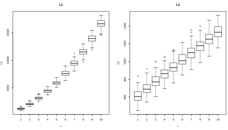
In the second experiment, we study the effect of the rankr on denoising error. To this end, we fix m = 2000, n = 1000, k = l = 50, σ = 1 and all the nonzero singular values of M as d1 = · · · = dr = 200. We vary r between 1 and 10. For each value of r, the U
and V matrices are generated in the same way as in the first experiment. Fig.2shows the boxplots of Lq(M,Mc) for q= 1 and 2 for the varying values of r out of 100 repetitions for
each of the ten values of r. It is noticeable that for the L1 loss, the denoising error grows quadratically as the rankr grows, while the trend is linear for theL2 loss. Both cases agree with Theorem4.
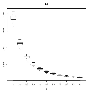
In the third experiment, we study the effect of the parameterq used in the loss function. To this end, we generated datasets in the same way as in the first experiment while fixing σ = 1. We take eleven different values of q ∈ [1,2] such that their reciprocals are equally spaced between 0.5 and 1. As Fig.3shows, the logarithm of the loss function scales linearly with 1/q. Again, this is in accordance with the error bound in Theorem4.
● ●
● ● ● ● ●
● ●
● ● ● ●
● ● ●
0.2 0.4 0.6 0.8 1 1.2 1.4 1.6 1.8 2
0
10000
20000
30000
40000
50000
60000
70000
L1
sigma
L1
● ● ● ● ●
● ●
● ● ●
● ● ●
● ● ●
0.2 0.4 0.6 0.8 1 1.2 1.4 1.6 1.8 2
0
1000
2000
3000
4000
L2
sigma
L2
Figure 1: Loss vs.σ: boxplots of 100 repetitions. Left panel: L1 loss. Right panel: L2 loss.
● ●
● ●
●
● ●
● ●
1 2 3 4 5 6 7 8 9 10
5000
10000
15000
L1
r
L1
● ●
● ●
● ●
● ●
● ●
●
1 2 3 4 5 6 7 8 9 10
600
800
1000
1200
1400
L2
r
L2
●
●
●
●
● ●
●
● ●
1 1.1 1.2 1.3 1.4 1.5 1.6 1.7 1.8 1.9 2
5000
10000
15000
20000
Lq
q
Lq
Figure 3: Loss vs.q: boxplots of 100 repetitions.
(k, l) (50, 50) (50, 200) (100, 200) (100, 50)
Average(L2(M,Mc)) 1133.03 2662.07 3598.69 1673.49
Standard error (5.96) (11.73) (12.84) (9.73)
Average
L2(M,cM)
(r+logm)(k+l)
0.64 0.60 0.68 0.63
Average(L1(M,Mc)) 19056.47 43035.95 65099.19 28347.12
Standard error (88.42) (172.39) (231.98) (146.07)
Average
L1(M,cM)
(r2+rlogm)(k+l)
1.08 0.98 1.23 1.07
Table 1: Average losses (with its standard error) and average rescaled losses of cM out of
100 repetitions for different sparsity levels.
their standard errors over 100 repetitions. Moreover, we report the rescaled average loss where the rescaling constant is chosen to ber2q−1(r+ logm)(k+l), the rate derived in
The-orem4. By the results reported in Table1, we see that for either loss function, the rescaled average losses are stable with respect to different sparsity levels specified by different values of kand l. Again, this agrees well with the earlier theoretical results.
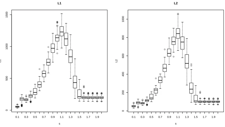
In the last experiment, we study the effect of “spikiness”, i.e., how the concentration of energy of the nonzero entries in M affects denoising. To this end, we fix m = 2000, n = 1000, k=l = 50, r = 1,d1 = 200 and σ = 1. In this case, U and V are both vectors. To vary the “spikiness”, we set all nonzero entries ofV to be equal and the nonzero entries of U as
Ui1 =Csi−1/s, fori= 1, . . . , k,
for a grid of twenty equally spacedsvalues in {0.1,0.2, . . . ,2}. Here, for any givens,Cs is
● ● ● ● ● ● ● ● ● ● ● ● ● ● ● ● ● ● ● ● ● ● ● ● ● ● ● ● ● ● ● ● ●●●● ●●●● ● ● ● ● ● ● ● ● ● ●
0.1 0.3 0.5 0.7 0.9 1.1 1.3 1.5 1.7 1.9
0 500 1000 1500 L1 s L1 ● ● ● ● ● ● ● ● ● ● ● ● ● ● ● ● ● ● ● ●●● ●●●● ● ● ● ● ● ● ● ● ● ●
0.1 0.3 0.5 0.7 0.9 1.1 1.3 1.5 1.7 1.9
0 200 400 600 800 1000 L2 s L2
Figure 4: Loss vs. “spikiness”: boxplots of 100 repetitions. Left panel: L1loss. Right panel: L2 loss.
entries in U decay to zero and the more concentrated the energy of the nonzero entries in U and hence inM. Fig.4 shows the boxplots ofLq(M,Mc) forq = 1 and 2 for the varying
values ofsout of 100 repetitions for each of the twenty values ofs. A somewhat surprising phenomenon is that the error is not monotone in “spikiness”. For both L1 and L2 losses, the errors first increase ass increases until they reach the peak whens= 1.1 and then the errors decay assfurther increases. Finally, they stabilize aftersbecomes 1.6 or larger. We feel that this intriguing phenomenon might be explained intuitively as the following. For small to medium values ofs, both the bias and the variance in the estimator increases with s. However, due to the additionall0 sparsity ofU, the bias starts to decrease aftersgrows larger than some critical value (1.1 in this simulation). Furthermore, when sgrows larger than another critical value (1.6 in this simulation), the estimator essentially estimates the entire nonzero block inMand the bias term vanishes, which explains the stabilization near the end of the curves in Fig. 4.
5. Discussion
In this section, we discuss two additional issues related to the present work.
in functionals (leading eigenvectors) of the covariance matrix. In addition, sparse PCA only deals with one set of sparse eigenvectors while the denoising problem studied here needs to deal with both left and right sparse singular vectors. In particular, even in the case of Schatten-2 (Frobenius) norm loss, the theoretical results of the present paper cannot be obtained directly from those for sparse PCA, such as those in Ma (2013), Cai et al. (2013a,b), etc.
Loss function In the present paper, we have considered the collection of squared Schatten-q norm for q ∈ [1,2] as possible loss functions. One of the referees raised the question whether it is possible to extend the results to the case of q < 1, where the loss function becomes a squared quasinorm1. This could serve as an interesting topic for future research. However, when q < 1, the quasinorm is no longer convex and so the technique for estab-lishing estimation lower bounds which was first laid out in Ma and Wu (2015) no longer applies directly.
6. Proofs
6.1 Proof of Theorem 2
The proof of Theorem2 relies on the following theorem, which is quoted without proof.
Theorem 8 (Theorem 2 in Ma and Sun (2014)) Let the observed X ∈ Rn×p,Y ∈
Rn×m be generated by the modelY=XA+ZwithZhaving i.i.d.N(0, σ2)entries. Suppose
for some absolute constant γ >1, the coefficient matrix A∈Rp×m belongs to
Θ(s, r, d, γ) ={A: rank(A) =r, γd≥σ1(A)≥ · · · ≥σr(A)≥d >0,|supp(A)| ≤s}.
Moreover, suppose the (2s)-sparse Riesz constants of the design matrix X satisfy K−1 ≤
κ−(2s) ≤ κ+(2s) ≤ K for some absolute constant K > 1. Then there exists a positive
constant c depending only on γ and κ+(2s) such that for all q∈[1,2],
inf b A
sup Θ E
Lq(A,Ab)≥cσ2
r2/q−1d 2 σ2
∧hr2/q(s+m) +r2/q−1slogep s
i
.
Proof [Proof of Theorem 2] To establish the lower bound, first consider the subset F1 ⊂
F(m, n, k, l, r, d, κ) where we further require supp(V) = [r]. Thus, except for the first r columns, all columns ofMare zeros. So, by a simple sufficiency argument, we may assume that n =l =r. In this case, the problem of estimating (the first r columns of) M under model (1) can be viewed as a special case of sparse reduced rank regression where the design matrix is the identity matrix Im. Note that the sparse Riesz constants for Im are all equal
to one. Therefore, Theorem8 implies that
inf c M
sup
F
ELq(M,Mc)≥inf
c M
sup
F1
ELq(M,Mc)≥c h
r2q−1d2∧
r2qk+r
2
q−1klogem
k
i
.
By symmetry, we also have
inf c M
sup
F E
Lq(M,cM)≥c h
r2q−1d2∧
r2ql+r
2
q−1llogen
l
i
.
We complete the proof by noting that for anya, b, c >0, (a∧b)∨(a∧c) =a∧(b∨c)a∧(b+c).
6.2 Proof of Theorem 4
To prove Theorem 4, we follow the oracle sequence approach developed in Ma (2013). Throughout the proof, we assume that σ = 1 is known. The case of general σ > 0 comes from obvious scaling arguments. In what follows, we first define the oracle sequence and introduce some preliminaries. Then we give an overview of the proof, which is divided into three steps. After the overview, the three steps are carried out in order, which then leads to the final proof of the theorem. Due to the space limit, proofs of intermediate results are omitted.
Preliminaries We first introduce some notation. For any matrix A, span(A) stands for the subspace spanned by the column vectors of A. If we were given the oracle knowledge of I = supp(U) and J = supp(V), then we can define an oracle version of the observed matrix as
e
X= (xij1i∈I1j∈J)∈Rm×n. (14)
With appropriate rearrangement of rows and columns, theI×J submatrix concentrates on the top-left corner. From now on, we assume that this is the case. We denote the singular value decomposition of Xby
e
X=
h
e
U Ue⊥ i
"
e
D 0
0 De⊥ # "
e
V0 (Ve⊥)0
#
, (15)
where Ue,De,Ve consist of the first r singular triples of Xe, and Ue⊥,De⊥,Ve⊥ contain the
remaining n−r triples (recall that we have assumed m≥n). In particular, the successive singular values ofXe are denoted by de1 ≥de2≥ · · · ≥den≥0.
With the oracle knowledge of I and J, we can define oracle versions of Algorithm 2 and Algorithm 1. In the oracle version of Algorithm 2, we replace the subsets I0 and J0 by Ie0 = I0 ∩I and Je0 = J0 ∩J, and the output matrices are denoted by Ue(0) and
e
V(0). In the oracle version of Algorithm 1, X is replaced by Xe and V(0) is replaced by e
V(0). The intermediate matrices obtained after each step within the loop are denoted by
e
U(t),mul,Ue(t),thr,Ue(t) and Ve(t),mul,Ve(t),thr,Ve(t), respectively. We note that for anyt, it is
guaranteed that
supp(Ue(t),thr) = supp(Ue(t))⊂I,
supp(Ve(t),thr) = supp(Ve(t))⊂J.
To investigate the properties of the oracle sequence, we will trace the evolution of the columns subspaces of Ue(t),mul,Ue(t), Ve(t),mul and Ve(t). To this end, denote ther canonical
angles (Golub and Van Loan, 1996) between span(Ue(t),mul) and span(Ue) by π/2≥φ
(t)
u,1 ≥
· · · ≥φ(u,rt) ≥0, and define
Moreover, denote the canonical angles between span(Ue(t)) and span(Ue) by π/2 ≥θ
(t)
u,1 ≥
· · · ≥θ(u,rt) ≥0, and let
sin Θ(ut)= diag(sinθu,(t)1, . . . ,sinθ(u,rt)). (17) The quantitiesφ(v,it), sin Φv(t),θ(v,it)and sin Θ
(t)
v are defined analogously. For any pair ofm×r
or-thonormal matricesW1andW2, let the canonical angles between span(W1) and span(W2) be π/2 ≥ θ1 ≥ · · · ≥ θr ≥ 0 and sin Θ = diag(sinθ1, . . . ,sinθr), then (Stewart and Sun,
1990)
ksin ΘkF = 1
√
2kW1W
0
1−W2W 0 2kF,
ksin Θkop =kW1W10 −W2W02kop.
(18)
Overview Given the oracle sequence defined as above, we divide the proof into three steps. First, we show that the output of the oracle version of Algorithm 2 gives a good initial value for the oracle version of Algorithm1. Next, we prove two recursive inequalities that characterize the evolution of the column subspaces of Ue(t) and Ve(t), and show that
after T iterates, the output of the oracle version of Algorithm 1 estimates M well. Last but not least, we show that with high probability the oracle estimating sequence and the actual estimating sequence are identical up to 3T iterates and thatTb∈[T,3T]. Therefore,
the actual estimating sequence inherits all the nice properties that can be claimed for the oracle sequence.
In what follows, we carry out the three steps in order.
Initialization We first investigate the properties ofXe,Ie0,Je0 and Ve(0).
Note that for any orthonormal matrix W, WW0 gives the projection matrix onto span(W). The following lemma quantifies the difference between the leading singular struc-tures of Xand M.
Lemma 9 With probability at least 1−m−2,
kUU−UeUekF,kVV−VeVekF≤
√
2r dr
√
k+√l+ 2plogm, (19)
and for any i∈[n],
|dei−di| ≤
√
k+
√
l+ 2plogm=o(dr), (20)
where the last equality holds under Condition 1.
Proof By symmetry, we only need to spell out the arguments forUin (19). By definition,
e
X=UDV0+Ze where (after reordering of the rows and the columns)Ze =
ZIJ 0
0 0
. Thus,
we have
kUU0−UeUe0kF≤
√
2rkUU0−UeUe0kop ≤
√
2r dr
Here, the first inequality holds since rank(UU0−UeUe0)≤2r and the last inequality is due
to Wedin’s sinθ theorem (Wedin, 1972). By the Davidson-Szarek bound (Davidson and Szarek,2001), with probability at least 1−m−2, kZekop =kZIJkop ≤
√
k+√l+ 2√logm. This completes the proof of (19).
On the other hand, Corollary 8.6.2 ofGolub and Van Loan(1996) implies that|dei−di| ≤
kZIJkop. Together with the above discussion, we obtain the first inequality in (20). The second inequality is a direct consequence of Condition 1. This completes the proof.
Next, we investigate the properties of the sets selected in Algorithm 2. For some uni-versal constants 0< a−<1< a+, define the following two deterministic sets
I±0 =ni∈[m] :kMi∗k2≥a∓α
p
nlogmo, J±0 =nj∈[n] :kM∗jk2≥a∓α
p
mlogmo.
(21)
Lemma 10 Let Condition 1 be satisfied, and let α ≥ 4, a− ≤ 201 and a+ ≥ 2 be fixed
constants. For sufficiently large values ofm andn, with probability at least1−O(m−2), we
have I−⊆Ie0⊆I+ and J−⊆Je0 ⊆J+, and soI0 =Ie0 and J0=Je0.
Proof By symmetry, we only show the proof forIe0 here. The arguments forJe0 are similar.
On the one hand, we have
P(I−0 *Ie0)≤ X
i∈I0
−
P
kXi∗k2 < n+α
p
nlogm
≤mP
χ2n(a+α
p
nlogm)< n+αpnlogm
≤m exp
−(a+−1)
2α2nlogm 4n+ 8a+α
√
nlogm
≤m exp(−3 logm) =m−2.
Here, the last inequality holds for fixeda+≥2,α≥4 and all sufficiently large (m, n) such that 2a+α
√
nlogm≤n/3, which is guaranteed by Condition1. On the other hand, for x= (1−a−)2α2nlogm
(2.1)2(n+2a−√nlogm), we have P(Ie0*I+0)≤
X
i∈(I0
+)c P
kXi∗k2 > n+α
p
nlogm
≤mP
χ2n(a−α
p
nlogm)> n+αpnlogm
≤mP
χ2n(a−α
p
nlogm)> n+ 2.1
q
(n+ 2α−
p
nlogm)x
≤mP
χ2n(a−α
p
nlogm)> n+ 2
q
(n+ 2α−
p
nlogm)x+ 2x
≤m exp (−x)
Here, the fourth inequality holds for fixed α ≥4, a− ≤ 201, and all sufficiently large (m, n)
such that n+ 2a−
√
nlogm ≥ 0.221(1−a−)2α
√
nlogm. The last inequality holds when, in addition, 0.952·16·n ≥ 3·(2.1)2 ·(n+ 2a−
√
nlogm), which is again guaranteed by Condition1.
Finally, when I−⊆Ie0 ⊆I+, we have I0 =Ie0 sinceI+ ⊂I.
The next lemma estimates the accuracy of the starting pointVe(0) for the oracle version
of Algorithm1.
Lemma 11 Let Condition1 be satisfied, and let α≥4and a+≥2 be fixed constants. For
sufficiently large values of m and n, uniformly over F(m, n, k, l, r, d, κ), with probability at
least 1−O(m−2), for a positive constant C that depends only onκ, a+ and α,
ksinΘe(0)v kF ≤
C d
h
r2k2nlogm1/4+ r2l2mlogm1/4
i
≤ 1
6.
Proof LetX(0)be the matrix defined in Step2of Algorithm2, but withI0andJ0replaced by Ie0 and Je0. Then we have
ksinΘe(0)v kF =
1
√
2kVe (0)
e
V(0)−VeVe0kF ≤
√
2r
√
2 kVe (0)
e
V(0)−VeVe0kop≤
√
r
e
dr
kXe −Xe(0)kop.
Here, the first equality is from (18). The second inequality holds since rank(Ve(0)Ve(0)− e
VVe0)≤2r, and the last inequality is due to Wedin’s sinθtheorem (Wedin,1972).
To further bound the rightmost side, we note thatXe(0) andXe are supported onIe0×Je0
and I×J respectively, withIe0×Je0 ⊂I×J. In addition, (I×J)\(Ie0×Je0) is the union of
two disjoint subsets (I\Ie0)×J and Ie0×(J\Je0). Thus, the triangle inequality leads to
kXe −Xe(0)kop ≤ kXe
I\Ie0,Jkop+k
e
X e
I0,J\Je0kop
≤ kUI\ e
I0,∗D(VJ∗)0kop+kUIe0∗D(VJ\Je0∗)
0k
op+kZI\Ie0,Jkop+kZIe0,J\Je0kop. (22)
We now bound each of the four terms in (22) separately. For the first term, on the event such that the conclusion of Lemma 10 holds, we have
kUI\Ie0,∗DV
0
Jkop≤ kDkopkVJ∗kopkUI\Ie0,∗kop ≤d1kUI\Ie0,∗kF≤
d1 dr
(a+α)1/2(k2nlogm)1/4. Here, the last inequality is due to I0
− ⊂Ie0, the definition of I−0 in (21), and the facts that
kMi∗k ≥ drkUi∗k for all i∈ [m] and that |I\Ie0| ≤ |I| ≤ k. By similar argument, on the
event such that the conclusion of Lemma 10 holds, we can bound the second term in (22) as
kU e
I0∗D(VJ\Je0∗)
0k
op ≤ kUIe0∗kopkDkopkVJ\Je0∗kop ≤d1kUkopkVJ\Je0∗kF ≤ d1
dr
To bound the last two terms, we first note that on the event such that the conclusion of Lemma10holds, both terms are upper bounded by kZIJkop. Together with the Davidson– Szarek bound (Davidson and Szarek, 2001), this implies that with probability at least 1−m−2,
kZI\ e
I0,Jkop+kZIe0,J\Je0kop ≤2kZIJkop ≤2
√
k+
√
l+ 2plogm
.
Assembling the last five displays and observe thatder≥0.9dr for sufficiently large values of
(m, n) on the event such that the conclusion of Lemma9, we obtain the first inequality in the conclusion. The second inequality is a direct consequence of Condition 1. This com-pletes the proof.
Evolution We now study how the column subspaces of Ue(t) and Ve(t) evolve over
itera-tions. To this end, let
ρ=der+1/der, (23)
wheredei denotes the ith singular value ofXe.
Proposition 12 For any t≥1, letxt=ksin Θ(ut)kF, yt=ksin Θ(vt)kF. Moreover, define ωu = (2der)−1
p
kγ2
u, ωv = (2der)−1
p
lγ2
v, ω=ωu∨ωv. (24)
Let Condition 1 be satisfied. Then for sufficiently large values of (m, n), on the event such
that the conclusions of Lemmas 9–11hold,
1) For any t≥1, if yt−1 <1, then
xtp1−(yt−1)2 ≤ρyt−1+ω
u, yt
p
1−(xt)2≤ρxt+ω
v. (25)
2) For any a∈(0,1/2], if
yt−1 ≤ 1.01ω
(1−a)(1−ρ), (26)
then so is xt. Otherwise,
xt≤yt−1[1−a(1−ρ)]. (27)
The same conclusions hold with the ordered pair (yt−1, xt) replaced by (xt, yt) in (26)–
(27).
Proof 1) In what follows, we focus on showing the first inequality in (25). The second inequality follows from essentially the same argument.
Let ut=ksin Φ(ut)kF. We first show that ut≤ ρy
t−1
p
Recall the SVD ofXe in (15). In addition, let the QR factorization ofUe(t),mul=Qe(t)Re(t),mul.
By definition, Ue(t),mul =XeVe(t−1). Premultiplying both sides by h
e
U Ue⊥ i0
, we obtain
"
e
D 0
0 De⊥
# "
e
V0Ve(t−1)
(Ve⊥)0Ve(t−1) #
=
"
e
U0Qe(t)
(Ue⊥)0Qe(t) #
e
R(t),mul.
In addition, let
"
e
U0Qe(t)
(Ue⊥)0Qe(t) #
=
O(t) W(t)
.
By the last two displays, we have
W(t)=De⊥(Ve⊥)0Ve(t−1)(Re(t),mul)−1 =De⊥
h
(Ve⊥)0Ve(t−1) i h
e
V0Ve(t−1) i−1
e
D−1hUe0Qe(t) i
.
Thus,
kW(t)kF≤ kDe⊥kopk(Ve⊥)0Ve(t−1)kFk[Ve0Ve(t−1)]−1kopkDe−1kopkUekopkQe(t)kop.
By Corollary 5.5.4 ofStewart and Sun(1990),kW(t)kF =ut,k(Ve⊥)0Ve(t−1)kF =yt−1.
More-over, by Section 12.4.3 of Golub and Van Loan (1996), k[Ve0Ve(t−1)]−1kop = 1/cosθ
(t−1)
v,r =
1/
q
1−(sinθ(v,rt−1))2 ≤1/ p
1−(yt−1)2. Here we have used the assumption that yt−1 <1. Together with the facts that kDe⊥kop =der+1, kDe−1kop =de−r1, kUekop =kQe(t)kop = 1, this
leads to (28).
Next, we show that
xt≤ut+p ωu
1−(yt−1)2. (29)
To this end, letwt=kQe(t)(Qe(t))0−Ue(t)(Ue(t))0kF. Then, by (18) and the triangle inequality,
we obtain
xt≤ut+√1
2w
t.
To bound wt, note that Wedin’s sinθtheorem (Wedin,1972) implies
wt≤ kUe
(t),mul−
e
U(t)kF
σr(Ue(t),mul)
.
In the oracle version,Ue(t),mulhas at mostknonzero rows, and sokUe(t),mul−Ue(t)kF≤ p
kγ2
u.
For any unit vector y ∈ span(Ve(t−1)), decompose y = y0+y1 where y0 ∈ span(Ve) and
y1 ∈ span(Ve⊥). Then by definition, ky0k ≥ cosθ (t−1)
v,1 ≥
p
1−(yt−1)2. Thus, for any unit vector x, kUe(t),mulxk2 = kXVe (t−1)xk2 = kXye k2 = kXy0e k2+kXy1e k2 ≥ kXy0e k2 =
kXeVeVe0y0k2≥(der)2ky0k2 ≥(der)2[1−(yt−1)2]. Hence,
σr(Ue(t),mul)≥ inf
kxk=1
kUe(t),mulxk ≥der p
Assembling the last three display, we obtain (29). Finally, the first inequality in (25) comes from (28), (29) and the triangle inequality.
2) Given (25), we have
xt≤ ρy
t−1+ω
p
1−(yt−1)2, and that y0 ≤ 1
6 ≤ 1
5(1−ρ)
2 for sufficiently large values of (m, n) due to Condition 1 and Lemma 9. The proof of part (2) then follows from the same argument as in the proof of Proposition 6.1 in Ma(2013).
Convergence We say that the oracle sequence hasconverged if
xt∨yt≤ 1.01ω
(1−m−1)(1−ρ). (30)
This choice is motivated by the observation that 11.01−ρω is the smallest possible value for xt and yt that Proposition 12 can lead to.
Proposition 13 Let Condition 1 be satisfied and T be defined in (12). For sufficiently
large values of(m, n), on the event such that the conclusions of Lemmas 9–11hold, it takes
at most T steps for the oracle sequence to converge in the sense of (30). For any t, let
e
P(ut) =Ue(t)(Ue(t))0 andPe
(t)
v =Ve(t)(Ve(t))0. Then there exists a constant C that depends only
onκ, such that for all t≥T,
kPe(ut)XePe(vt)−UeDeVek2F ≤C kγ2u+lγv2
.
Proof To prove the first claim, we rely on claim (2) of Proposition 12. Without loss of generality, assume that m= 2ν for some integer ν ≥1. So ν = logm/log 2. Let t1 be the number of iterations needed to ensure thatxt∨yt≤ 1.01ω
(1−1 2)(1−ρ)
. Note that when (26) does
not hold, (27) ensures that
yt≤yt−1[1−a(1−ρ)]2, xt≤xt−1[1−a(1−ρ)]2. (31) Thus, it suffices to have
1−1
2(1−ρ)
2t1 ≥ 1.01ω
(1−1 2)(1−ρ)
, i.e., 2t1|log(1−12(1−ρ))| ≥log(1− 1
2)(1−ρ)/(1.01ω). Since |log(1−x)| ≥x for all x∈(0,1), it suffices to set t1 =
1 1−ρlog
1
2(1−ρ) 1.01ω =
1 +o(1) 2 log
d2r kγ2
u∨lγv2
.
Next, lett2−t1be the number of additional iterations needed to achievext∨yt≤1.01ω/[(1− 1
4)(1−ρ)]
2. Before this is achieved, (31) is satisfied witha= 1
4. So it suffices to have [1− 1 4(1− ρ)]2(t2−t1) ≤(1−1
2)/(1− 1
4), which is guaranteed if t2−t1 ≥ 2
1−ρ[log(1−
1
4)−log(1− 1 2)]. Recursively, we define ti for i = 3, . . . , ν, such that xti, yti ≤ 1.01ω/[(1−2−i)(1−ρ)].
Repeating the above argument shows that it suffices to have ti−ti−1= 2
i−1
1−ρ[log(1−2
−i)−
log(1−2−(i−1))] fori= 3, . . . , ν. Therefore, if we let tν−t1=
ν+ 1/2 2(1−ρ) =
(1 +o(1)) logm 2 log 2 ≥
ν X
i=1
2i−1 1−ρ
h
log(1−2−i)−log(1−2−(i−1))
i
then xt∨yt ≤1.01ω/[(1−m−1)(1−ρ)] for allt ≥tν. We complete the proof of the first
claim by noting that T ≥tν for sufficiently largem,nunder Condition 1.
To prove the second claim, letPeu =UeUe0 and Pev=VeVe0. Then we have
kPe(ut)XePev(t)−UeDeVekF=kPe(ut)XePe(vt)−PeuXePevkF (32)
≤ k(Pe(ut)−Peu)XePe(vt)kF+kPeuXe(Pev(t)−Pev)kF
≤ kPe(ut)−PeukFkXekopkPe(vt)kop+kPe(vt)−PevkFkXekopkPeukop
=de1
kPe(ut)−PeukF+kPe(vt)−PevkF
(33)
≤Cpkγ2
u+
p
lγ2
v
. (34)
Here, the equality (32) is due to the definitions of Peu, Pev and the fact that Ue, De and
e
V consist of the first r singular values and vectors of Xe. The equality (33) holds since
kXekop =de1 and kPeukop =kPe
(t)
v kop = 1 as both are projection matrices. Finally, the in-equality (34) holds since kPe
(t)
u −PeukF =
√
2xt and kPe
(t)
v −PevkF =
√
2yt due to (18), the definitions in (24) and (30), and the fact that on the event such that (20) holds,de1/der≤2κ
when m andn are sufficiently large. This completes the proof.
Remark 14 It is worth noting that the conclusions of Proposition 12 and Proposition 13
hold for any γu>0 and γv >0, though they will be used later with the specific choice ofγu
and γv in (10).
Proof of Upper Bounds We are now in the position to prove Theorem4. To this end, we need to establish the equivalence between the oracle and the actual estimating sequences. The following lemma shows that with high probability, the oracle sequence and the actual sequence are identical up to 3T iterates.
Lemma 15 Let γu and γv be defined as in (10) with some fixed constant β ≥ 4 and let
Condition1 be satisfied. For sufficiently largemandn, with probability at least1−O(m−2),
for all 1≤t≤3T, UI(tc)∗=0, V
(t)
Jc∗ =0, and so U(t)=Ue(t) and V(t)=Ve(t).
Proof First of all, by Lemma10, with probability at least 1−O(m−2),J0=
e
J0 ⊂J + ⊂J, and so Ve(0) =V(0). Define eventE(0) ={V(0)=Ve(0)}.
We now focus on the first iteration. Define event
Eu(1) =nkZi∗Ve(0)k< γu,∀i∈Ic o
.
OnE(0)∩Eu(1), for anyi∈Ic,Ui(1)∗ ,mul=Xi∗V(0)=Zi∗Ve(0). Thus,kU
(1),mul
i∗ k< γu and so
U(1)i∗ ,thr =0 for all i∈Ic. This further implies U(1)Ic∗ =0 and U(1) =Ue(1). Further define
event
Ev(1) =nk(Z∗j)0Ue(1)k< γv,∀j∈Jc o
Then by similar argument, on the eventE0∩Eu(1)∩Ev(1), we haveV(1)Jc∗=0andV(1) =Ve(1).
We now bound the probability of (Eu(1))c. Without loss of generality, let J ⊂[l]. Note
that for anyj ∈J,i∈Ic,Ve(0) depends onZij only through kZIcjk2 in the selection ofJe0
in the oracle version of Algorithm2. Therefore,Ve(0) is independent of
Zij
kZIcjk. Letk
0 =|Ic|
andY1, . . . Ylbe i.i.d.χk0 random variables independent ofZ. For anyi∈Icandj∈[l], let
ˇ Zij =Yj
Zij
kZIcjk,
and ˇZi[l]= ( ˇZi1, . . . ,Zˇil) ∈R1×l. Since supp(Ve(0))⊂J ⊂ [l] on the event E(0), we obtain
that for anyi∈Ic,Zi∗Ve(0) =Zi[l]Ve(0) = ˇZi[l]Ve(0)+ (Zi[l]−Zˇi[l])Ve(0). Thus,
kZi∗Ve(0)k ≤ kZˇi[l]Ve
(0)
[l]∗k+k(Zi[l]−Zˇi[l])Ve
(0)
[l]∗k ≤ kZˇi[l]Ve
(0)
[l]∗k+kZi[l]−Zˇi[l]kkVe
(0) [l]∗kop.
For the first term on the rightmost side, since ˇZi[l]is independent ofVe(0),kZˇi[l]Ve
(0) [l]∗k
2 ∼χ2
r,
and so by Lemma17, with probability at least 1−O(m−β),
kZˇi[l]Ve
(0) [l]∗k
2 ≤r+ 2p
βrlogm+ 2βlogm.
For the second term, we first note that kVe
(0)
[l]∗kop = 1 since it has orthonormal columns.
Moreover, ˇZi[l]−Zi[l]=Zi[l]diag
Y1
kZIc1k −1, . . . ,
Y1
kZIclk −1
. Thus,
kZˇi[l]−Zi[l]k ≤ kZi[l]kmax
j∈[l]
Yj
kZIcjk
−1 .
By Lemma17, with probability at least 1−O(m−β),
kZi[l]k2≤l+ 2
p
βllogm+ 2βlogm.
By Lemma18, for anyj ∈[l], with probability at least 1−O(m−(β+1)),
Yj
kZIcjk
−1 ≤
Yj2
kZIcjk2
−1
≤4·1.01·
r
(β+ 1) logm
k0 .
Here, the last inequality holds for sufficient large values of m and n, since Condition 1 implies that (logm)/k0 =o(1). By the union bound, with probability at least 1−O(m−β), for sufficient large values ofm and n,
kZˇi[l]−Zi[l]k ≤0.01plogm ,
since Condition1ensures thatl/k0 =o(1). Assembling the last six displays, we obtain that for any β >1, with probability at least 1−O(m−β),
kZi∗Ve(0)k ≤ q
Applying the union bound again, we obtain that whenβ ≥4 in (10),
P
n
(Eu(1))co≤O(m−3). (35) Similarly, for anyj ∈Jc,Ue(1)depends onZij only throughkZiJck. Therefore, by analogous
arguments, we also obtain (35) for (Ev1)c with any fixed β ≥4. Turn to subsequent iterations, we further define events
Eu(t)=nkZi∗Ve(t−1)k< γu,∀i∈Ic o
, Ev(t)=nk(Z∗j)0Ue(t)k< γv,∀j ∈Jc o
, t= 2, . . . ,3T.
Iterating the above arguments, we obtain that on the event E(0)∩(∩3T
t=1E
(t)
u )∩(∩3t=1T E
(t)
v ),
U(Itc)∗=0,V
(t)
Jc∗ =0, and soU(t)=Ue(t)andV(t) =Ve(t). Moreover, by similar argument to
that for (35), we can bound eachP{(Eu(t))c}and P{(Ev(t))c}byO(m−3) for allt= 2, . . . ,3T
with any fixed β≥4 in (10). Finally, under Condition 1,T =O(m), and so
P
n
E(0)∩(∩t3=1T Eu(t))∩(∩3t=1T Ev(t))o= 1−O(m−2). This completes the proof.
Lemma 16 Let Tb be defined in (11). With probability at least 1−O(m−2), T ≤Tb≤3T.
Proof By definition (10) and (12), we have
T ≤ 1.01
2
logm log 2 + log
d2r γ2
.
On the other hand, note that 1/log 2≥1.44 and that log(k∨l)≤logmunder the assump-tion thatm≥n, and hence
T ≥ 1.01
2
logm
log 2 −logm+ log d2r γ2
≥ 1.01
2
0.44 logm+ log d 2
r
γ2
.
On the other hand, on the event such that the conclusions of Lemmas9–11 hold, we have
|d(0)r −dr| ≤ |d(0)r −der|+|der−dr|
=|de(0)r −der|+|der−dr|
≤ kXe(0)−Xekop+o(dr)
=o(dr).
Hence for sufficiently large values of m and n, logγ2 > 1 and with probability at least 1−O(m−2),|log(d(0)
r )2/logd2r−1| ≤0.01. When the above inequalities all hold, we obtain b
T ∈[T,3T].
Proof [Proof of Theorem4] Note that on the events such that the conclusions of Lemmas 9–16 hold, we have
kMc−MkF
=kPb(uTb)XPb(vTb)−UDV0kF
≤ kPb(
b
T)
u XPb(
b
T)
v −UeDeVe0kF+kUeDeVe0−UDV0kF
=kPe(uTb)XePe(vTb)−PeuXePevkF+kPeuXePev−PuMPvkF
≤ kPe(
b
T)
u XePe(
b
T)
v −PeuXePevkF+kPeuXePev−PeuMPevkF
+kPeuMPev−PuMPvkF.
Here, the first and the second inequalities are both due to the triangle inequality. The second equality is due to Lemma16 and the facts that supp(Ue(t))⊂I, supp(Ve(t))⊂J and
thatUe and Ve collect the first r left and right singular vectors of Xe.
We now bound each of the three terms on the rightmost side of the last display. First, on the event such that the conclusions of Proposition13 and Lemma16 hold, we have
kPe(uTb)XePev(Tb)−PeuXePevkF≤C p
kγ2
u+lγv2.
Next, by similar argument to that leading to the conclusion of Lemma11, with probability at least 1−O(m−2)
kPeuXePev−PeuMPevkF ≤ kXe −MkF=kZIJkF
≤√rkZIJkop
≤√r(
√
k+
√
l+ 2plogm).
Last but not least,
kPeuMPev−PuMPvkF
≤ k(Peu−Pu)MPevkF+kPuM(Pev−Pv)kF
≤d1(kPeu−PukF+kPev−PvkF)
≤κ√r(
√
k+
√
l+ 2plogm).
Assembling the last four displays, we complete the proof for the case of Frobenius norm, i.e., q = 2. To obtain the result for all q ∈ [1,2), simply note that for any matrix A,
kAksq ≤(rank(A))1q−
1 2kAk
6.3 Proof of Proposition 7
Proof [Proof of Proposition 7] Without loss of generality, assume that σ = 1. We first show thatbr≤r with probability at least 1−O(m
−2). To this end, note that P{br > r}=P
σr+1(XI0J0)> δ|I0||J0| ≤P
max
|A|=|I0|,|B|=|J0|σr+1(XAB)> δ|A||B|
≤
m X
i=r+1
n X
j=r+1
P
max
|A|=i,|B|=jσr+1(XAB)> δij
.
By the interlacing property of singular values, we know that for Z, a m ×n standard Gaussian random matrix,
max
|A|=i,|B|=jσr+1(XAB) st
< max
|A|=i−r,|B|=j−rσ1(ZAB) st
< max
|A|=i,|B|=jσ1(ZAB),
where<st means stochastically smaller. Together with the union bound, this implies
P
max
|A|=i,|B|=jσr+1(XAB)> δij
≤
m i
n j
P{σ1(ZAB)> δij}
≤em
i
ien
j
j
exp
−ilogem
i −jlog em
j −4 logm
=m−4.
Here, the second inequality is due to pk≤(ep/k)k for anyk∈[p] and the Davidson-Szarek bound (Davidson and Szarek,2001). Asn≤m under Condition 1, we obtain
P{br > r} ≤ m X
i=r+1
n X
j=r+1
m−4 ≤m−2.
To show thatbr≥rwith probability at least 1−O(m−2), we note that on the event such that the conclusions of Lemmas9–11 hold, σr(XI0J0) = σr(Xe0) =de
(0)
r . So by the triangle
inequality, the conclusion of Lemma9 and the proof of Lemma 11, we obtain that
σr(XI0J0) =der(0)≥dr− kX−Xekop− kXe −Xe0kop≥dr/4> δkl,
where the second last and the last inequalities hold under Condition1 for sufficiently large values ofmand n. Note that on the event such that the conclusion of Lemma 10holds, we have |I0| ≤k and |J0| ≤l and so δ|I0||J0|≤δkl. This completes the proof.
Acknowledgments
Appendix A. Appendix
Lemma 17 (Lemma 8.1 in Birg´e (2001)) Let X follow the non-central chi square
dis-tributionχ2ν(δ) with degrees of freedomν and non-centrality parameter δ≥0. Then for any
x >0,
P
n
X ≥ν+δ+ 2p(ν+ 2δ)x+ 2x
o
≤e−x,
P
n
X ≤ν+δ−2p(ν+ 2δ)xo≤e−x.
Lemma 18 Let X andY be two independent χ2ν random variables. Then for anyx >0,
P
(
X Y −1
≤ 4
p
x/ν(1 +px/ν) 1−2px/ν
)
≥1−4e−x.
Proof By the triangle inequality,
X Y −1
≤ 1
|Y|(|X−ν|+|Y −ν|).
By Lemma17, for anyx >0, each of the following holds with probability at least 1−2e−x:
|X−ν| ≤2√νx+ 2x,
|Y −ν| ≤2√νx+ 2x, and |Y| ≥ν−2√νx.
Assembling the last two displays, we complete the proof.
References
L. Birg´e. An alternative point of view on Lepski’s method, volume 36 of Lecture
Notes-Monograph Series, pages 113–133. Institute of Mathematical Statistics, 2001.
F. Bunea, Y. She, and M.H. Wegkamp. Optimal selection of reduced rank estimators of high-dimensional matrices. The Annals of Statistics, 39(2):1282–1309, 2011.
F. Bunea, Y. She, and M.H. Wegkamp. Joint variable and rank selection for parsimonious estimation of high dimensional matrices. The Annals of Statistics, 40:2359–2388, 2012.
C. Butucea and Yu.I. Ingster. Detection of a sparse submatrix of a high-dimensional noisy matrix. Bernoulli, 19(5B):2652–2688, 2013.
T.T. Cai, Z. Ma, and Y. Wu. Sparse PCA: Optimal rates and adaptive estimation. The
Annals of Statistics, 41(6):3074–3110, 2013a.
T.T. Cai, X. Li, and Z. Ma. Optimal rates of convergence for noisy sparse phase retrieval via thresholded Wirtinger flow. arXiv preprint arXiv:1506.03382, 2015.
E.J. Cand`es and Y. Plan. Matrix completion with noise. Proceedings of the IEEE, 98(6): 925–936, 2010.
E.J. Cand`es and B. Recht. Exact matrix completion via convex optimization. Foundations
of Computational mathematics, 9(6):717–772, 2009.
G. Chen, P.F. Sullivan, and M.R. Kosorok. Biclustering with heterogeneous variance.
Pro-ceedings of the National Academy of Sciences, 110(30):12253–12258, 2013.
K.R. Davidson and S. Szarek.Handbook on the Geometry of Banach Spaces, volume 1, chap-ter Local operator theory, random matrices and Banach spaces, pages 317–366. Elsevier Science, 2001.
D.L. Donoho and M. Gavish. Minimax risk of matrix denoising by singular value thresh-olding. The Annals of Statistics, 42(6):2413–2440, 2014.
J. Fan and R. Li. Variable selection via nonconcave penalized likelihood and its oracle properties. Journal of the American Statistical Association, 96:1348–1360, 2001.
C. Gao, Y. Lu, Z. Ma, and H. H. Zhou. Optimal estimation and completion of matrices with biclustering structures. arXiv preprint arXiv:1512.00150, 2015.
G. H. Golub and C. F. Van Loan. Matrix computations. Johns Hopkins University Press, 3rd edition, 1996.
R.H. Keshavan, A. Montanari, and S. Oh. Matrix completion from noisy entries. The
Journal of Machine Learning Research, 11:2057–2078, 2010.
V. Koltchinskii, K. Lounici, and A.B. Tsybakov. Nuclear-norm penalization and optimal rates for noisy low-rank matrix completion. The Annals of Statistics, 39(5):2302–2329, 2011.
K. Lee, Y. Wu, and Y. Bresler. Near optimal compressed sensing of sparse rank-one matrices via sparse power factorization. arXiv preprint arXiv:1312.0525, 2013.
M. Lee, H. Shen, J.Z. Huang, and J.S. Marron. Biclustering via sparse singular value decomposition. Biometrics, 66:1087–1095, 2010.
X. Li and V. Voroninski. Sparse signal recovery from quadratic measurements via convex programming. SIAM Journal on Mathematical Analysis, 45(5):3019–3033, 2013.
K. Lounici, M. Pontil, S. Van De Geer, and A. B. Tsybakov. Oracle inequalities and optimal inference under group sparsity. The Annals of Statistics, 39(4):2164–2204, 2011.
Z. Ma. Sparse principal component analysis and iterative thresholding. The Annals of
Z. Ma and T. Sun. Adaptive sparse reduced-rank regression. arXiv preprint
arXiv:1403.1922, 2014.
Z. Ma and Y. Wu. Volume ratio, sparsity, and minimaxity under unitarily invariant norms.
IEEE Transactions on Information Theory, To appear, 2015.
S. Negahban and M.J. Wainwright. Estimation of (near) low-rank matrices with noise and high-dimensional scaling. The Annals of Statistics, 39(2):1069–1097, 2011.
S. Oymak and B. Hassibi. Asymptotically exact denoising in relation to compressed sensing.
arXiv preprint arXiv:1305.2714, 2013.
S. Oymak, A. Jalali, M. Fazel, and B. Hassibi. Noisy estimation of simultaneously structured models: Limitations of convex relaxation. In Decision and Control (CDC), 2013 IEEE
52nd Annual Conference on, pages 6019–6024. IEEE, 2013.
S. Oymak, A. Jalali, M. Fazel, Y.C. Eldar, and B. Hassibi. Simultaneously structured models with application to sparse and low-rank matrices. IEEE Transactions on Information
Theory, 61(5):2886–2908, 2015.
A.A. Shabalin, V.J. Weigman, C.M. Perou, and A.B. Nobel. Finding large average subma-trices in high dimensional data. The Annals of Applied Statistics, 3:985–1012, 2009.
Y. Shechtman, Y.C. Eldar, A. Szameit, and M. Segev. Sparsity based sub-wavelength imaging with partially incoherent light via quadratic compressed sensing. Optics Express, 19(16):14807–14822, 2011.
G.W. Stewart and J.-G. Sun. Matrix Perturbation Theory. Computer science and scientific computing. Academic Press, 1990.
X. Sun and A.B. Nobel. On the maximal size of large-average and anova-fit submatrices in a gaussian random matrix. Bernoulli, 19(1):275–294, 2013.
P.-A. Wedin. Perturbation bounds in connection with singular value decomposition. BIT, 12:99–111, 1972.
D. Yang, Z. Ma, and A. Buja. A sparse singular value decomposition method for high-dimensional data. Journal of Computational and Graphical Statistics, 23(4):923–942, 2014.
M. Yuan and Y. Lin. Model selection and estimation in regression with grouped variables.
Journal of the Royal Statistical Society: Series B, 68(1):49–67, 2006.
X.-T. Yuan and T. Zhang. Truncated power method for sparse eigenvalue problems.Journal
of Machine Learning Research, 14:899–925, 2013.
C.H. Zhang. Nearly unbiased variable selection under minimax concave penalty.The Annals