Efficient Algorithms for Conditional Independence Inference

Efficient Algorithms for Conditional Independence Inference

Remco Bouckaert∗ [email protected]

Department of Computer Science University of Waikato

Hamilton 3240, New Zealand

Raymond Hemmecke [email protected]

Silvia Lindner [email protected]

Zentrum Mathematik

Technische Universtit¨at Munich Boltzmannstrasse 3

85747 Garching, Germany

Milan Studen´y [email protected]

Institute of Information Theory and Automation of the ASCR Pod Vod´arenskou vˇeˇz´ı 4

18208 Prague, Czech Republic

Editor: Rina Dechter

Abstract

The topic of the paper is computer testing of (probabilistic) conditional independence (CI) impli-cations by an algebraic method of structural imsets. The basic idea is to transform (sets of) CI statements into certain integral vectors and to verify by a computer the corresponding algebraic re-lation between the vectors, called the independence implication. We interpret the previous methods for computer testing of this implication from the point of view of polyhedral geometry. However, the main contribution of the paper is a new method, based on linear programming (LP). The new method overcomes the limitation of former methods to the number of involved variables. We re-call/describe the theoretical basis for all four methods involved in our computational experiments, whose aim was to compare the efficiency of the algorithms. The experiments show that the LP method is clearly the fastest one. As an example of possible application of such algorithms we show that testing inclusion of Bayesian network structures or whether a CI statement is encoded in an acyclic directed graph can be done by the algebraic method.

Keywords: conditional independence inference, linear programming approach

1. Introduction

First, we explain the motivation and mention some previous work. Then we describe the aim and structure of the paper.

1.1 Motivation

Conditional independence (CI) is a highly important concept in statistics and artificial intelligence.

Properties of probabilistic CI provide theoretical justification for the method of local computation

(Cowel et al., 1999) which is at the core of probabilistic expert systems (Jensen, 2001), successfully applied in numerous areas. The importance of CI is given by its interpretation in terms of relevance

among symptoms or variables in consideration (Pearl, 1988); that’s why it is crucial in probabilistic

reasoning. Traditional methods for describing (statistical models of) CI structures use graphs whose nodes correspond to variables in consideration; it leads to popular graphical models (Lauritzen, 1996).

Formal properties of probabilistic CI and the attempts to describe probabilistic CI inference in terms of mathematical logic have been traditional research topics since the late 1970’s. Basic prop-erties of CI, now known as the semi-graphoid propprop-erties, were accentuated in statistics by Dawid (1979). Pearl (1988) interpreted those properties, formulated in the form of simple implications be-tween CI statements, as axioms for the relevance relation. Moreover, Pearl proposed to view graphs as “inference engines” devised for efficient representing and manipulating relevance relationships. His idea (see Pearl, 1988, page 14) was to use an input list of CI statements to construct a graph and then, by using a special graphical separation criterion, to read from the graph additional CI statements, implied by the input list through the axioms. The goal of such inference procedures is to enable one to determine, at any state of knowledge, what information is relevant to the task at hand and what can be ignored.

Pearl’s intention led him to a conjecture that CI inference for discrete probabilistic distributions can be characterized by the semi-graphoid properties. The conjecture was refuted in Studen´y (1989); actually, it has been shown later that there is no finite system of properties of semi-graphoid type characterizing (discrete probabilistic) CI inference (Studen´y, 1992). Thus, the question of computer testing of CI inference became a topic of research interest.

In Studen´y (2005), the method of structural imsets has been proposed as a non-graphical alge-braic device for describing probabilistic CI structures; its advantage over graphical approaches is that it allows one to describe any discrete probabilistic CI structure. The idea is to use, instead of graphs, certain special integral vectors (of high dimension), called imsets, as tools for describing CI structures and implementing the “inference engine” for CI implication. This is because the cor-responding algebraic relation between structural imsets, called independence implication, gives a sufficient condition for (probabilistic) CI inference. The topic of this paper is computer testing of this implication. The intended use is

• computer testing of implications between CI statements, and

• checking equivalence of structural imsets by an algebraic method.

1.2 Some Former Algorithms

Given structural imsets u and v (over a set of variables N), the intuitive meaning of the implication

u⇀v (≡ u independence implies v) is that the CI structure induced by u contains the CI structure

induced by v. In Studen´y (2005, § 6.2) two algebraic characterizations of the relation u⇀v were

given. They established the theoretical basis for the first-generation algorithms for computer testing of u⇀v. The limitation of these algorithms is that to implement them fully one needs some

addi-tional information obtainable as the result of computations, which were performed only for|N| ≤5 (Studen´y, Bouckaert, and Koˇcka, 2000).

The theoretical aspects of their implementation were analyzed in Studen´y (2004), while their practical implementations were described in detail in Bouckaert and Studen´y (2007). Basically, there are two algorithms, which can be interpreted as mutually complementary procedures. One of them, based on so-called “direct” characterization of u⇀v (see Studen´y, 2005, § 6.2.1), is suitable

to confirm the implication; that’s why it was called the verification algorithm in Bouckaert and Studen´y (2007). The other algorithm, based on so-called “skeletal” characterization of u⇀v (see

Studen´y, 2005, § 6.2.2), fits to disproving the implication; that’s why it was named the falsification

algorithm.

The main idea of Bouckaert and Studen´y (2007) was to combine both algorithms to get a more effective tool. Owing to the computations from Studen´y et al. (2000), the implemented versions of both these algorithms are guaranteed to give a decisive answer to any independence implication problem for|N| ≤5. Nevertheless, the combined version has also been implemented for|N|=6, although without a guaranteed response to each implication problem. Recently, the first-generation algorithms from Bouckaert and Studen´y (2007) have been applied (in a modified form) in connec-tion with the lattice-theoretic approach to CI inference (Niepert, van Gucht, and Gyssens, 2008).

1.3 Aim of the Paper

In this paper, we bring a new view on the problem of testing CI inference. First, we interpret the previous methods from the point of view of polyhedral geometry. Second, this geometric in-terpretation and the linear programming approach lead to new methods and, consequently, to the second-generation algorithms for testing CI inference, which appear to be more efficient than the first-generation algorithms.

More specifically, the geometric view has recently helped to solve an open problem that was very closely related to the topic of CI inference (see Studen´y, 2005, Question 7). It was the question whether every structural imset is a combinatorial imset, that is, whether it can be written as the sum of elementary imsets (= imsets corresponding to elementary CI statements). The question has been answered negatively in Hemmecke et al. (2008), where an example of a structural imset over 5 variables was found that is not combinatorial.

This fact naturally leads to a more advanced question motivated by the topic of CI inference: what is the so-called Hilbert basis of the cone generated by standard imsets (cf., Studen´y, 2005, Theme 10). A recent achievement is that the Hilbert basis for |N|=5 has been found as a result of computations by Bruns et al. (2010). This makes it possible to design two modifications of the verification algorithm for 5 variables. In fact, the CI inference problem is transformed to testing whether a given imset is combinatorial, respectively structural.

Another important idea brought by this paper is that every testing u⇀v task can be re-formulated

this implication already in Studen´y (2004, § 5). However, in the present paper, we re-formulate this implication problem in a different way. The LP approach has the following advantages:

• it allows one to go far beyond the limit of 5 variables,

• the second-generation algorithms are much faster than the first-generation ones,

• the re-formulation makes it possible to apply highly effective software packages developed to solve LP problems.

The goal of this paper is to describe the idea of the new approach, the corresponding algorithms and the experiments, whose aim was to compare the new algorithms (with the old ones).

Moreover, to give an example of the possible use of the algorithms we prove a result related to learning Bayesian networks. We characterize the inclusion of BN structures in terms of their algebraic representatives, standard imsets. Given acyclic directed graphs G and H over N, we show that the BN structure induced by H is contained in the one induced by G iff the difference uG−uHof

their standard imsets is a combinatorial imset, which happens iff it is a structural imset. Thus, testing the inclusion can be transformed to testing combinatorial imsets (or structural ones). A consequence of this observation is an elegant algebraic procedure for reading CI statements represented in a standard imset uG, a kind of counterpart of the graphical separation criterion. Since the standard

imset uGis quite simple we have reasons to conjecture that our procedure can be implemented with

polynomial complexity with respect to|N|.

1.4 Structure of the Paper

Section 2 is devoted to the terminology for CI inference using structural imsets, while basic concepts from polyhedral geometry are recalled in Section 3. In Section 4, the methods we are using are explained and, in Section 5, the experiments we performed are described. In Conclusions we discuss the perspectives and formulate some open problems. Appendices contain some proofs, a table of types of the Hilbert basis elements for 5 variables, an illustrative example and a comment on possible interpretation of the LP method.

2. Concepts Concerning CI Inference

The symbol N will be used to denote a non-empty finite set of variables in consideration. Given disjoint sets of variables A,B⊆N, the juxtaposition AB will denote their union.

2.1 Conditional Independence

Let P be a discrete probability distribution over N specified by its density p :XN →[0,1], where XN ≡∏i∈NXi is the joint sample space, a product of non-empty finite individual sample spaces.

Given A⊆N and x∈XN, let xAdenote the respective marginal configuration of x and pAthe marginal

density of p; by convention p/0(−) =1. Given pairwise disjoint A,B,C ⊆N, we say that A is conditionally independent of B given C with respect to P if

We write A⊥⊥B|C[P]then and call it a CI statement with respect to P; if P is not material we just use the symbol A⊥⊥B|C. The CI structure induced by P consists of all CI statements valid with

respect to P.

Now, let L be a set of CI statements, called an input list, and t a CI statement outside L. We say

L probabilistically implies t if, for every discrete probability distribution P, whenever all statements

in L are valid with respect to P then t is valid with respect to P, too. Classic examples of valid probabilistic CI implications are the semi-graphoid properties (Pearl, 1988):

Symmetry A⊥⊥B|C =⇒ B⊥⊥A|C,

Decomposition A⊥⊥BD|C =⇒ A⊥⊥D|C,

Weak union A⊥⊥BD|C =⇒ A⊥⊥B|DC,

Contraction A⊥⊥B|DC & A⊥⊥D|C =⇒ A⊥⊥BD|C.

A CI statement A⊥⊥B|C is called elementary if both A and B are singletons and it is called trivial

if either A=/0or B=/0. Since trivial statements are always valid, it follows from the semi-graphoid properties that, for any discrete probability distribution P, the CI structure induced by P is uniquely determined by the list of elementary CI statements valid with respect to P.

2.2 Imsets

An imset over N is an integer-valued function on the power set of N, denoted by

P

(N)in the rest of the paper.1 It can be viewed as a vector whose components, indexed by subsets of N, are integers. An easy example is the zero imset, denoted by 0; another simple example is the identifierδA of a

subset A⊆N:

δA(S) =

1 if S=A,

0 if S⊆N,S6=A.

An imset associated with a CI statement A⊥⊥B|C is then the combination

uhA,B|Ci≡δABC+δC−δAC−δBC.

The class of elementary imsets (over N), denoted by

E

(N), consists of imsets associated with ele-mentary CI statements (over N).

A combinatorial imset is an imset u that can directly be decomposed into elementary imsets, that is,

u=

∑

w∈E(N)

kw·w for some kw∈Z+.

We denote the class of combinatorial imsets over N by

C

(N).

An imset u over N will be called structural if there exists n∈N_{such that the multiple n·u is a}

combinatorial imset, that is,

n·u=

∑

w∈E(N)

kw·w for some n∈N,kw∈Z+.

In other words, a structural imset is an imset which is a combination of elementary ones with non-negative rational coefficients. The class of structural imsets over N will be denoted by

S

(N); this

class of imsets is intended to describe CI structures. Clearly,

E

(N)⊆

C

(N)⊆

S

(N). One has

C

(N) =

S

(N)for|N| ≤4 (Studen´y, 1991), but

S

(N)6=

C

(N)for|N|=5 (Hemmecke et al., 2008). However, one can show (see Studen´y, 2005, Lemma 6.3) that there exists a smallest n∗∈N, depending on|N|, such that u∈

S

(N)⇔n∗·u∈

C

(N)for every imset u over N. One has n∗=1 for

|N| ≤4 (Studen´y, 1991) and one of the news brought by this paper is that n∗=2 for|N|=5 (see Proposition 6 in Appendix B). An open question is what is the exact value of n∗ for every|N|(cf., Studen´y, 2005, Theme 11).

2.3 Independence Implication

Let u,v be structural imsets over N. We say that u independence implies v and write u⇀v if there

exists k∈N_{such that k·u−v is a structural imset:}

u⇀v iff ∃k∈N _k·u−v∈

S

(N). (1)

Now, given u∈

S

(N)the corresponding CI structure

M

(u)consists of all CI statements A⊥⊥B|C

such that u⇀uhA,B|Ci. The importance of structural imsets follows from the fact that, for every discrete probability distribution P over N, there exists u∈

S

(N)such that the CI structure induced by P coincides with

M

(u)(use Studen´y, 2005, Theorem 5.2).

An equivalent characterization of independence implication is as follows. A real set function

m :

P

(N)→R_{is called supermodular iff}

m(C∪D) +m(C∩D)≥m(C) +m(D) for every C,D⊆N.

Such a function can be viewed as a real vector whose components are indexed by subsets of N. The

scalar product of m and an imset u over N is then

hm,ui ≡

∑

S⊆N

m(S)·u(S).

The dual definition of independence implication is this (see Studen´y, 2005, Lemma 6.2): one has

u⇀v iff, for every supermodular function m over N,

hm,ui=0 =⇒ hm,vi=0. (2)

The independence implication can be viewed as a sufficient condition for probabilistic CI im-plication. More specifically, given an input list L of CI statements, let us “translate” every statement

s in L into the associated imset usand introduce a combinatorial imset uL≡∑s∈Lus. Then one has:

Proposition 1 Let L be an input list of CI statements and t another CI statement over N. If uL⇀ut

then L probabilistically implies t.

The reader may be interested in whether there exists a limit for the factor k in (1). If we assume that the “input” u is a combinatorial imset and the “output” v an elementary one then such a limit exists. One can show (cf., Studen´y, 2005, Lemma 6.4) that the least k∗∈Nexists such that

u⇀v iff k∗·u−v∈

S

(N).

It depends on|N|: k∗=1 for|N| ≤4 and k∗=7 for |N|=5 (Studen´y et al., 2000). It is an open question what is the exact value of k∗for|N| ≥6 (cf., Studen´y, 2005, Theme 12).

2.4 Bayesian Network Translation

Bayesian networks (Pearl, 1988; Neapolitan, 2004) can be interpreted as graphical models of CI

structures assigned to acyclic directed graphs. More specifically, given an acyclic directed graph G having N as the set of its nodes, the corresponding graphical separation criterion (for the definition see Lauritzen, 1996, § 3.2.2) defines the collection

I

(G)of CI restrictions given by G. The corre-sponding statistical model then consists of probability distributions onXN that are Markovian with respect to G, that is, satisfy those CI restrictions. Given two acyclic directed graphs G and H over N, we say they are independence equivalent if

I

(G) =

I

(H); it essentially means they define the same statistical model.

Given an acyclic directed graph G over N, the standard imset for G, denoted by uG, is given by

the formula

uG =δN−δ/0+

∑

i∈N

{δ_pa

G(i)−δ{i}∪paG(i)}, (3) where pa_G(i)≡ {j∈N; j→i in G} denotes the set of parents of a node i in G. Lemma 7.1 in Studen´y (2005) says that uG is always a combinatorial imset and

M

(uG) =

I

(G). Thus, the

graphical separation criterion applied to G can be replaced by an algebraic criterion applied to

uG. Moreover, Corollary 7.1 in Studen´y (2005) adds that uG=uH iff G and H are independence

equivalent. That means, the standard imset is a unique representative of the equivalence class of graphs.

Note that uG need not be the only combinatorial imset defining

I

(G); it is the simplest such

imset, a kind of “standard” representative. Using standard imsets we can easily characterize the inclusion for Bayesian networks:

Proposition 2 Let G and H be acyclic directed graphs over N. Then

I

(H)⊆

I

(G)if and only if

uG−uH∈

C

(N), which is also equivalent to uG−uH∈

S

(N).

Proof The equivalence

I

(H)⊆

I

(G)⇔uG−uH∈

C

(N)is proved in (Studen´y, 2005, Lemma 8.6).

Clearly, uG−uH∈

C

(N) implies uG−uH ∈

S

(N). Conversely, if uG−uH∈

S

(N) then, by (1), uG⇀uH and it makes no problem to show

M

(uH)⊆

M

(uG). This means

I

(H)⊆

I

(G).

acyclic directed graphs G and H. Of course, a different situation is with testing independence equivalence, in which case a simple graphical characterization and algorithms are available.

Proposition 2 has the following consequence, which allows one to replace the graphical separa-tion criterion by testing whether an imset is combinatorial.

Corollary 3 Given an acyclic directed graph G over N, the class

I

(G)coincides with the collection of CI statements A⊥⊥B|C such that uG−uhA,B|Ci∈

C

(N), respectively uG−uhA,B|Ci∈

S

(N).

Proof It is enough to construct, for every CI statements A⊥⊥B|C, an acyclic directed graph H

such that uhA,B|Ci=uH. To this end, consider a total order of nodes in N in which C is followed A, B and N\ABC, direct edges of the complete undirected graph over N according to this order and

remove the arrows between A and B.

Of course, as mentioned above, there are elegant graphical separation criteria for testing whether a CI statement is represented in an acyclic directed graph. There are no doubts that these criteria can be implemented with polynomial complexity in|N|(see Geiger, Verma, and Pearl, 1989) and that they are also appropriate for human users. However, our method proposed in Corollary 3 may appear to be suitable for computer testing, in particular in the situation when the Bayesian network structure is internally represented in a computer by the standard imset, as suggested in Studen´y, Vomlel, and Hemmecke (2010).

3. Basic Concepts from Polyhedral Geometry

Here we recall some well-known concepts and facts from the theory of convex polyhedra. Proofs can be found in textbooks on linear programming, for example Schrijver (1986).

Vectors are regarded as column vectors. Given two vectors x,y, their scalar product will be denoted either byhx,yior, using matrix multiplication notation, by x⊺_{y, where x}⊺_{is the transpose}

of x. The inequality x≤y is meant in all components, and0, respectively1, is a vector all whose components are zeros, respectively ones.

3.1 Polyhedra, Polyhedral Cones and Farkas’ Lemma

Systems of linear inequalities appear in many areas of mathematics. Let A be a d×n-matrix and b

a d-vector. The set of all solutions inRn_{to the linear system Ax≤b is called a polyhedron. If the}

defining matrix A and the right-hand side vector b are rational, the polyhedron is said to be rational. Polyhedra defined via homogeneous inequalities Ax≤0are called polyhedral cones.

A non-trivial fundamental result in polyhedral geometry states that every polyhedral coneCcan equivalently be introduced as the conical hull cone(V)of finitely many pointsV⊆Rn_{, that is, the}

set of all finite conical combinations∑tλt·vt(withλt≥0 for all t) of elements vt∈V(see Schrijver,

1986, Corollary 7.1a). If the polyhedral cone is rational then it is the conical hull of finitely many

rational points. A classic algorithmic task is to change between the inner descriptionC=cone(V) and the outer descriptionC={x∈Rn_{; Ax≤0}, and back. Standard software packages that allow}

one to switch between both descriptions are for example 4TI2 (4ti2 team, 2008), CDD (Fukuda, 2008), or CONVEX(Franz, 2009).

check whether Av≤b and thus, v∈P. However, is there also a simple certificate for the case that

P= /0? Indeed, there is such a certificate (see Schrijver, 1986, Corollary 7.1e):

Lemma 4 (Farkas’ lemma) The system Ax≤b is solvable iff every u∈Rd _{with A}⊺_{u=0, u≥0} satisfies u⊺_b≥0.

Thus, any u∈Rd _{satisfying A}⊺_{u=0, u≥0 and u}⊺_{b<0 gives a certificate that Pis empty.}

Indeed, given x∈P, write 0=0⊺_{x= (A}⊺_u)⊺_{x= (u}⊺_A)x=u⊺_(Ax)≤u⊺_{b<0 to get a contradiction.}

To decide using a computer whether P6=/0 or not, we can make use of well-developed tools from the theory of linear programming (see below, Section 3.4).

3.2 Dimension and Faces of a Polyhedron

The dimension dim(P)of a polyhedronP⊆Rn_{is the dimension of its affine hull aff(}P), which is the set of all finite affine combinations∑_tλt·vt (withλt ∈R for all t and∑tλt =1) of elements

vt ∈P. By convention, the dimension of the empty set is−1. A polyhedron is full-dimensional if

dim(P) =n.

Given v∈Rn_andα_∈R_{, we call the inequalityhv},xi ≤αvalid for a polyhedronP⊆Rn_{if it is}

satisfied for every x∈P. If the inequalityhv,xi ≤αis valid for the polyhedronP, we call the set

F=P∩ {x∈Rn_;hv,xi=α_{}a face ofP.}

The sets /0andPare always faces of a polyhedronP, defined by the valid inequalitiesh0,xi ≤1 andh0,xi ≤0, respectively. Every polyhedronPhas only finitely many faces and all of them are polyhedra, too (see Schrijver, 1986, § 8.3). They can be classified by their dimension. Faces of dimension 0 are points in Rn_{, called vertices. Faces of dimension 1 are called edges: these are}

either line-segments, half-lines or lines. Faces of dimension dim(P)−1 are called facets.

If a polyhedron is full-dimensional then facet-defining inequalities establish a unique (up to positive scalar factors) inclusion-minimal inequality system definingP (for details see Schrijver, 1986, § 8.4). Since every (proper) face F of P is the intersection of facets containing it, facets implicitly determine all faces.

A polyhedron P={x; Ax≤b}is pointed if the only vector y with Ay=0is the zero vector y=0 (see Schrijver, 1986, § 8.2). A non-empty pointed polyhedron has at least one vertex. A pointed polyhedral coneChas just one vertex0, its edges are half-lines, called extreme rays. Non-zero representatives of the extreme rays ofCthen provide its inclusion-minimal inner description (Schrijver, 1986, § 8.8).

3.3 Hilbert Basis

A lattice point (inRn_{) is an integral vector x∈}Zn_{, that is, a vector whose components are integers.}

By a Hilbert basis of a rational polyhedral coneC(see Schrijver, 1986, § 16.4) is meant a finite setH⊆Cof lattice points such that every lattice point inCis a non-negative integer linear combi-nation of elements inH. A relevant result in polyhedral geometry (Schrijver, 1986, Theorem 16.4) says that every rational polyhedral cone possesses a Hilbert basis. If the cone is in addition pointed, there is a unique inclusion-minimal Hilbert basis. Clearly, any Hilbert basis ofChas to include the above mentioned normalized representatives of extreme rays ofC.

Again, it is a challenging algorithmic task to compute the minimal integral Hilbert basis of a given (pointed) rational polyhedral cone. However, there are a few software packages that allow to do so in some simpler cases, for example 4TI2 (4ti2 team, 2008) or NORMALIZ(Bruns, Ichim, and S¨oger, 2009).

3.4 LP Problems and the Simplex Method

A linear programming (LP) problem is the task to maximize/minimize a linear function x7→ hc,xi, where c∈Rn_{, over a polyhedron}P={x∈Rn_{; Ax≤b}. A classic tool to deal with this problem is}

the simplex method. Nevertheless, it is not the aim to describe here the details of this method; they can be found in textbooks on linear programming; for example Schrijver (1986, Chapter 11).

We just recall its main features to explain the geometric interpretation. The plain version of the simplex method (see Schrijver, 1986, § 11.1) assumes one has a vertex of (a pointed polyhedron)

P as a starting iteration. The basic idea is to move from vertex to vertex along the edges of P

until an optimal vertex is reached or an edge is found on which the linear function is unbounded. Each particular variant of the simplex method uses a special pivoting operation to choose the next iteration, which should have a better value of the linear objective function than the previous one.

However, it may be the case that one is not sure whether the polyhedronPis non-empty. Then the simplex method has two phases. In Phase I, one finds at least one x∈P, called a feasible vertex

solution, provided that it exists, or one concludes that P= /0 otherwise. If a feasible solution is available, Phase II consists of finding an optimal solution as mentioned above. A standard trick to deal with Phase I is to re-formulate it as an auxiliary LP problem, in which a feasible vertex solution is known.

For example, consider the task to optimize a linear function over a special polyhedron of the formQ={x∈Rn_{; Ax=b,x≥0}, where A∈}Rd×n_{and b∈}Rd_{, which task is, in fact, equivalent to}

the general case (see Schrijver, 1986, § 7.4). Moreover, one can assume without loss of generality b≥0 here.2Then the auxiliary LP problem is as follows:

min{ h1,zi; (x,z)∈Rn+d_{,Ax+z=b, x≥0,z≥0}. (4)}

This LP problem has the vector(0,b) as a feasible vertex solution3 and it has the property that its optimal value h1,zi is 0 iff(x,z) = (x,0) and x∈Q. Thus, testing whether the polyhedronQ is non-empty can be done in this way.

4. Methods

In this section, we describe a few methods that can be used to test CI inference. The task is as follows. An input list L of elementary CI statements and another elementary CI statement t over

2. Indeed, if the i-th component of b is negative, one can replace the i-th row of A and the i-th component of b with their multiples by−1.

N are given and the goal is to decide whether uL⇀ut (cf., Proposition 1). We are going to give a

computational comparison of these methods for|N|=5 in Section 5.1 to see which of them is the fastest.

4.1 Method 1: using Skeletal Characterization

This is the first ever implemented method for testing independence implication (Studen´y et al., 2000, § 7.4). The motivation source for this method was the dual definition (2) of independence implication in terms of supermodular functions (see Section 2.3). The point is that, in (2), written in contrapositive form as4

hm,vi>0 =⇒ hm,ui>0,

one can limit oneself toℓ-standardized supermodular functions m :

P

(N)→R_{, that is, to those that}

satisfy m(S) =0 if|S| ≤1. This is a pointed rational polyhedral cone. The class of normalized integral representatives of its extreme rays was called theℓ-skeleton in Studen´y (2005) and denoted

by

K

⋄ ℓ(N).

The skeletal characterization of the implication u⇀v, for u,v∈

S

(N), is as follows:

∀m∈

K

⋄_ℓ(N) hm,vi>0 =⇒ hm,ui>0 (5)

(see Studen´y, 2005, Lemma 6.2). Theℓ-skeleton was computed for|N|=5 (Studen´y et al., 2000): it consists of 117978 imsets, which break into 1319 permutational types.

Thus, the corresponding algorithm consists in checking whether each of the implications in (5) is valid or not. To disprove the implication u⇀v it is enough to find at least one m∈

K

⋄

ℓ(N) violating (5); to confirm it one has to check that all of them are valid. By ordering the elements of theℓ-skeleton such that those m∈

K

⋄

ℓ(N)which are more likely to cause violation are tried earlier one can speed up the disproval (but not the confirmation). This suggested to sort elements of

K

⋄

ℓ(N) on the basis of zeros in{hm,wi; w∈

E

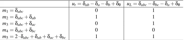
(N)}(for details see Bouckaert and Studen´y, 2007, § 3.1).

Example 1 To illustrate the method consider a trivial example with N ={a,b,c}: take the input L={a⊥⊥b|c, a⊥⊥c|/0}and t : a⊥⊥b|/0. We already know by semi-graphoid properties that L probabilistically implies t (see Section 2.1). However, the aim of this example is to get this conclusion through Proposition 1 (see Section 2.3) using the skeletal characterization. We have

uL=uha,b|ci+uha,c|/0i=δabc−δbc−δa+δ/0 and ut =uha,b|/0i=δab−δa−δb+δ/0.

In the case of 3 variables, theℓ-skeleton has 5 elements, listed in rows of Table 1. The columns in the table correspond to structural imsets ut and uL, the items are corresponding scalar products. The condition (5) evidently holds for v=ut and u=uL. Thus, uL⇀ut.

The interpretation of the method from the point of view of polyhedral geometry is as follows. The independence implication can equivalently be defined in terms of (inclusion of) facets of the cone

R

(N)≡cone(

E

(N)), the cone spanned by elementary imsets. Let Fudenote the face of

R

(N)

generated by u∈

S

(N)⊆

R

(N), that is, the least face of

R

(N)containing u (≡the intersection of all faces of

R

(N) containing u). Then, for u,v∈

S

(N), one has u⇀v iff the face Fu contains v,

which means, Fv⊆Fu(see Studen´y, 2005, Remark 6.2).

ut=δab−δa−δb+δ/0 uL=δabc−δbc−δa+δ/0

m1=δabc 0 1

m2=δabc+δab 1 1

m3=δabc+δac 0 1

m4=δabc+δbc 0 0

m5=2·δabc+δab+δac+δbc 1 1

Table 1: Scalar products with elements of

K

⋄

ℓ(N)for N={a,b,c}.

The method is based on the computation of all facets of the cone

R

(N). These facets correspond to the extreme rays of the (dual) cone ofℓ-standardized supermodular functions. Thus, basically, one is checking whether every facet containing Fualso contains Fv. The problem with this approach

is that it can hardly be extended beyond five variables because computing these facets seems to be computationally infeasible for|N| ≥6.

4.2 Method 2: Racing Algorithms

The idea of the paper (Bouckaert and Studen´y, 2007) was to combine two algorithms for testing the independence implication u⇀v. One of them, called the verification algorithm, was based on (1)

and appeared to be suitable to confirm the implication provided it holds. However, it may spend a long time before it gives a response if the implication does not hold. The other algorithm, called the falsification algorithm and based on (2), was designed to disprove the implication if it does not hold. However, it is not able to confirm u⇀v provided it holds.

The combined procedure starts with two threads, the verification one and the falsification one. Once one thread finds its proof, it stops the other and returns its outcome. This approach makes it possible to go beyond 5 variables, but may not give a decisive response (in reasonable time) to some complex implication problems. On the other hand, empirical evidence from Bouckaert and Studen´y (2007) suggests that this method is, on average, faster than the method described in Section 4.1.

4.2.1 VERIFICATION: DECOMPOSING INTOELEMENTARYIMSETS

Consider a combinatorial imset u∈

C

(N), an elementary imset v∈

E

(N) and the task to decide whether u⇀v. That is, by (1), testing whether k·u−v is a structural imset for some k∈N_{. Observe}

that (1) is equivalent to

∃l∈N _l·u−v∈

C

(N). (6)

Indeed,

C

(N)⊆

S

(N) gives (6)⇒(1). Now, (1) implies that n·(k·u−v) is a combinatorial imset for some k,n∈N_{(see Section 2.2). As(n−1)·v∈}

C

(N), it gives(n·k)·u−v∈

C

(N). Moreover, it follows from concluding remarks in Sections 2.2 and 2.3 that n∗·k∗is an upper limit for l in (6). In general, we do not know what is the least such upper limit for l. Even in case|N|=5, we only know it is a number between 7 (see Studen´y et al., 2000) and 14=2·7=n∗·k∗.

The characterization (6) allows one to transform testing independence implication to the task to decide whether a given candidate imset y=l·u−v is combinatorial. A combinatorial imset y

may have many decompositions y=∑_w∈E(N)kw·w, kw∈Z+into elementary imsets. However, the

number∑w∈E(N)kwof summands, called the degree of y, is the same for any such decomposition

y, the search space, the tree of potential decompositions, is known. This space could be big, but it

can be limited by introducing additional sanity checks, which allow one to cut off some blind alleys in the tree. Moreover, the search can be guided by suitable heuristics and this can speed up the resulting algorithm (for details see Bouckaert and Studen´y, 2007, § 3.2).

The decomposition itself is quite fast, but what can slow down the whole procedure is the factor

l from (6), depending on a particular pair u,v. The point is that the degree of a candidate imset y=l·u−v grows (linearly) with l; consequently, the size of the corresponding tree of possible

decompositions grows exponentially with l. Typically, if u⇀v holds then one often finds a

decom-position of y with l=1. However, for|N|=5, there are a few cases when the decomposition of y exists for 1<l≤7 and not for l−1 (for examples see Studen´y et al., 2000, § 4.3). In these cases and also when u⇀v does not hold one has to search through a huge space, which makes the method

infeasible for efficient disproving implications.

Example 2 Consider N={a,b,c,d}, the input list

L={a⊥⊥b|c,a⊥⊥c|d, a⊥⊥d|b, b⊥⊥c|ad}, (7)

and another CI statement t : a⊥⊥c|b. We are going to show uL⇀ut by the decomposition method. Actually, we show that (6) holds with l=1. More specifically, we have

uL = uha,b|ci+uha,c|di+uha,d|bi+uhb,c|adi

= δabcd+δabc−δab−δac−δbc−δbd−δcd+δb+δc+δd,

and, as ut =δabc−δab−δbc+δb, we know that

y≡1·uL−ut=δabcd−δac−δbd−δcd+δc+δd.

The task is to test whether y is a combinatorial imset. If this is the case then the degree of y must be 3, which means we search for a decomposition into elementary imsets with 3 summands. Clearly, at least one summand v has to satisfy v(abcd)>0. There are 6 elementary imsets over{a,b,c,d} with this property and two of them are excluded by sanity checks. For example, for v′=uhc,d|abiand

y′=y−v′one has−1=∑_{c,d}⊆Ty′(T)<0, which is impossible for a combinatorial imset in place

of y′. However, if we subtract ˜v=uha,b|cdithen

˜

y=y−v˜=δacd+δbcd−δac−δbd−2·δcd+δc+δd

is a good direction. Again, at least one of two summands v in the searched decomposition of ˜y must satisfy v(acd)>0 and the choice v=uha,d|cileads to the final decomposition

y=u_ha,b|cdi+uha,d|ci+uhb,c|di.

Thus, the implication uL⇀ut has been confirmed by the decomposition method.

To explain the geometric interpretation (of the method) note that the cone

R

(N) =cone(

E

(N)) is slightly special. The lattice points in this cone are just structural imsets.5 Moreover, there exists

a hyperplane in RP(N) _{which intersects all extreme rays of}

R

(N) just in its normalized integral representatives

E

(N)and these are the only lattice points in the intersection of this hyperplane with

R

(N). In particular, every structural imset belongs to one of parallel hyperplanes (to this basic one) and its “degree” says how far it is from the origin (= zero imset). Now, the condition (1) means that at least one multiple of u (by k∈N_{) has the property that it remains a lattice point within the cone}

R

(N)even if v is subtracted. The condition (6) is a minor modification of (1): it requires a multiple of u minus v is a sum of elementary imsets (with possible repetition). The algorithm, therefore, looks for the decomposition and the degree (of the candidate imset y) serves as the measure of its complexity.

4.2.2 FALSIFICATION: RANDOMLYGENERATINGSUPERMODULARFUNCTIONS

Falsification is based on the characterization (2). To disprove the implication u⇀v it is enough to

find a supermodular function m :

P

(N)→R_{such thathm,ui=0 andhm,vi>0. Actually, one can}

limit oneself toℓ-standardized integer-valued supermodular functions, that is, supermodular imsets. These imsets have a special form which allows one to generate them randomly. The idea is

• to randomly generate a collection of subsets of N,

• to assign them randomly selected positive integer values (and the zero values to remaining sets), and

• to modify the resulting function to make it a supermodular imset.

The details of this procedure can be found in Bouckaert and Studen´y (2007, § 3.3). The procedure allows one to disprove (= falsify) the implication u⇀v even for|N| ≥6, but it is clearly not able to confirm it provided it holds. Therefore, it has to be combined with a verification procedure.

Example 3 Consider N={a,b,c,d}and the same input list (7) as in Example 2, but a different CI statement t : b⊥⊥c|a to be derived. If our random procedure generates the supermodular imset

m=2·δabcd+δabc+δabd+δacd+2·δbcd+δbc+δbd+δcd,

then one can observe thathm,uLi=0 whilehm,uhb,c|aii=1. In particular, by (2), the respective

implication is not valid:¬(uL⇀uhb,c|ai).

The geometric interpretation of the algorithm is similar to the interpretation of the method from Section 4.1. Supermodular functions correspond to faces of the cone

R

(N). Thus, the procedure consists in random generating faces of

R

(N)and the aim to find a face of

R

(N)which contains u but not v.

4.3 Method 3: Decomposition via Hilbert Basis

An alternative to testing whether an imset is combinatorial is testing whether it is structural. Since structural imsets coincide with the lattice points in the cone

R

(N)≡cone(

E

(N)), each of them can be written as a sum (with possible repetition) of the elements of the Hilbert basis

H

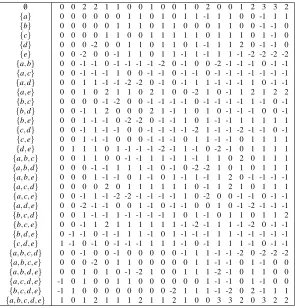
(N)of the cone

Computation of the Hilbert basis is a very hard task. Recently, the Hilbert basis of

R

(N) for

|N|=5 has been obtained as a result of sophisticated computations (Bruns et al., 2010). In Appendix B we provide a list of its representatives. Altogether, the obtained Hilbert basis of

R

(N)has 1300 elements, falling into 35 (permutation equivalence) types.

Thus, having the Hilbert basis of

R

(N) at hand, one can test the independence implication

u⇀v for u,v∈

S

(N)through (1): the task is to find out whether there exists a decomposition of

y≡k·u−v into Hilbert basis elements for some k∈N_{. This is analogous to the decomposition}

approach from Section 4.2.1, where the set of elementary imsets

E

(N)was used instead of

H

(N). Thus, the interpretation of this new method is the same, the difference is that we have now a wider class of leaves of the (potential) decomposition tree. On the other hand, the advantage of the Hilbert basis decomposition for|N|=5 should be that, in some complex cases, a much simpler decomposition of y may exist that involves also the elements of

H

(N)\

E

(N)(simpler = with a less number of summands). We are also sure that the upper limit for the constant k is only k∗=7. In particular, the depth of the tree of potential decompositions should be smaller, while the tree itself is expected to be wider.

4.4 Method 4: Linear Programming

The basic idea is to re-formulate (the definition of) independence implication in terms of the (pointed rational polyhedral) cone

R

(N)≡cone(

E

(N))spanned by elementary imsets. More specifically, given u,v∈

S

(N), the condition (1) can be expressed in this way:

u⇀v iff ∃k∈[0,∞) k·u−v∈

R

(N). (8)

Indeed, since

S

(N)⊆

R

(N)the implication (1)⇒(8) is evident. Conversely, provided (8) holds with

k, it holds with any k′≥k because

R

(N)is a cone and(k′−k)·u∈

R

(N). Therefore, there exists

k′∈N_{with k}′_·u−v∈

R

(N). As k′·u−v is an imset, it belongs to

S

(N), and (1) holds.

The geometric interpretation of the condition (8) is clear. It means that the ray (= half-line) with the origin in−v and the direction given by u intersects the cone

R

(N). The point is that testing whether this happens can be viewed as an LP problem:

Lemma 5 Given u,v∈

S

(N)one has u⇀v iff the system of equalities

∑

w∈E(N)

λw·w(S)−k·u(S) =−v(S) for any S⊆N, (9)

has a non-negative solution inλw, w∈

E

(N)and k.

Proof The cone

R

(N) consists of conic combinations of representatives of its extreme rays, that is, of elementary imsets. Thus, (8) can be re-written as the requirement for the existence of k≥0 andλw≥0 with k·u−v=∑w∈E(N)λw·w. This imset equality, specified for any S⊆N, yields (9).

Non-negative solutions to (9) form a polyhedron of the typeQ={x; Ax=b,x≥0}, A∈Rd×n_,

b∈Rd_{. Indeed, the rows of A correspond to subsets of N, while the columns to elementary imsets}

and the factor k. Thus, d=|

P

(N)|=2|N|and n=|

E

(N)|+1= |N₂|

(n+d)-dimensional space. An illustrative example of the application of this LP method in the case

|N|=3 is given in Appendix C.

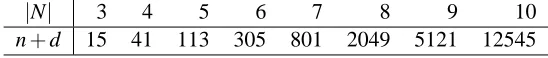
The advantage of this approach is that it is not limited to a particular number of variables as the previous ones. To get an impression of the implication problem complexity at hand, let us have a look at Table 2. Clearly, these (comparably small) linear programs should be solvable quickly in practice. We give computational evidence to this claim in Section 5.2. Another comment is that this LP method can be interpreted as a kind of decomposition procedure (analogous to the one from Section 4.2.1); see Appendix D for an explanation.

|N| 3 4 5 6 7 8 9 10

n+d 15 41 113 305 801 2049 5121 12545

Table 2: The dimensions of LP problems to be solved in order to decide u⇀v.

Let us finally note that there are alternative ways to re-formulate testing of u ⇀v as an LP

problem. For example, consider the cone ofℓ-standardized supermodular functions. We know the outer description of this (pointed) cone:

K

_ℓ(N) ={m∈RP(N)_{; m(S) =0 for|S| ≤1, hm,wi ≥0 for w∈}

E

(N)}.

Since, in (2), one can limit oneself toℓ-standardized supermodular functions, u⇀v is equivalent to

the requirement

sup{hm,vi; m∈

K

_ℓ(N),hm,ui=0} =0. (10)

This is an LP problem with a feasible region.6 Thus, Phase II of the simplex method can be applied to solve it. Note that (10), mentioned in Studen´y (2004, § 5), can be viewed, after appropriate modifications, as the dual LP problem to (9) in the sense of the LP theory; however, we omit the details in this paper.

5. Experiments

In this section, we describe the results of our computational experiments. We performed two sepa-rate bunches of experiments. One of them was done in New Zealand and the aim was to compare various methods in case|N|=5 (see Section 5.1).

As the result was that the LP method performs best in case|N|=5, the aim of the other group of experiments (see Section 5.2), done in Germany, was to test the LP approach in case|N|>5. These latter experiments were based on the commercial optimization software CPLEX (IBM Ilog team, 2009).

5.1 Comparison for Five Variables

Empirical evaluation of the methods can give insight in the practical behavior of the various meth-ods. First, we considered the case of five variables, so that we can compare the new methods with techniques based on skeletal representations (see Section 4.1). The experimental set up from Bouck-aert and Studen´y (2007) was used for the five-variable tests. In short, a thousand random input lists

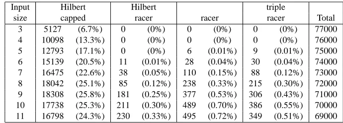
containing 3, up to 11 elementary CI statements were generated and, for each elementary CI state-ment outside the input list, it was verified whether it was implicated or not. So, the thousand 3-input cases result in verification of a thousand times the total number of elementary CI statements (80 for 5 variables) minus the 3 statements already given in the input list, that is, 1000×(80−3) =77000 inference problems. Table 3 lists the numbers of inference problems in its last column.

The algorithms considered were:

• Skeletal algorithm and sorted skeletal algorithm (see Section 4.1).

• Racing algorithms (see Section 4.2). There are situations where both the verification and the falsification algorithm perform poor, resulting in unacceptable running times. These outliers distort the typical behavior of the algorithm, so we put a cap on total calculation time and re-port the number of problems where a solution is not found within this deadline as the number of unresolved cases in Table 3.

• Hilbert basis (HB) decomposition algorithm (see Section 4.3). Initial experimentation showed

that the HB approach is very good at verifying the implication. However, when a CI state-ment is not implied, it takes a long time to traverse the search space. So, the average time for the HB approach is expected to be very poor. Again, we capped the allowed time for the algorithm to run and when no solution was found within that time the problem was as marked unresolved.

• The observation that the HB algorithm performs well for implication but poor on falsification immediately gives rise to another algorithm where the HB decomposition algorithm and fal-sification algorithm are raced against each other. This algorithm is called the Hilbert racer. Like the racer algorithm, this algorithm was time constrained.

• Now we have two algorithms that appear to perform well for verification, it is natural to combine them with the falsifier and thus get a three horse race. This algorithm is called the

triple racer, and it is time constrained as well.

• The last algorithm under consideration is the LP method described in Section 4.4.

Input Hilbert Hilbert triple

size capped racer racer racer Total

3 5127 (6.7%) 0 (0%) 0 (0%) 0 (0%) 77000

4 10098 (13.3%) 0 (0%) 0 (0%) 0 (0%) 76000

5 12793 (17.1%) 0 (0%) 6 (0.01%) 9 (0.01%) 75000

6 15139 (20.5%) 11 (0.01%) 28 (0.04%) 30 (0.04%) 74000 7 16475 (22.6%) 38 (0.05%) 110 (0.15%) 88 (0.12%) 73000 8 18042 (25.1%) 85 (0.12%) 238 (0.33%) 215 (0.30%) 72000 9 18308 (25.8%) 181 (0.25%) 377 (0.53%) 306 (0.43%) 71000 10 17738 (25.3%) 211 (0.30%) 489 (0.70%) 386 (0.55%) 70000 11 16798 (24.3%) 230 (0.33%) 495 (0.72%) 349 (0.51%) 69000

Table 3: Numbers of inference problems that were not resolved due to time-outs.

5.1.1 RESULTS ANDDISCUSSION

Table 3 shows the number of unresolved cases when time was capped at 1 second per problem. Only the algorithms that did not resolve all problems are shown there. The numbers in brackets are percentages, the last column the total number of problems for a particular input size.

Given the total number of problems (around 70 thousand per input size) this restricted calcu-lation took around 20 hours per input size. Clearly, the HB decomposition method when capped leaves a large proportion of implication problems unresolved, up to a quarter for the larger input sizes.

Combining the HB algorithm with the falsification algorithm reduces the number of unresolved problems to less than a third of a percent. Comparing the Hilbert racer with the original racer al-gorithm shows that more problems are resolved in the time available, so the HB decomposition algorithm appears to perform better at resolving problems. Finally, the triple racer, which combines both algorithms, performs in between the two algorithms in terms of number of unresolved prob-lems. At first sight, one would expect the triple racer to perform at least as good as the Hilbert racer, however, since the test was run on a dual core processor instead of a machine with at least three cores, the various algorithms were too busy battling for processor access and lost time to make the deadline.

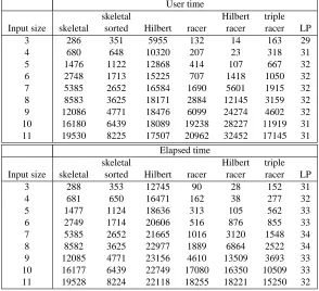
User time

skeletal Hilbert triple

Input size skeletal sorted Hilbert racer racer racer LP

3 286 351 5955 132 14 163 29

4 680 648 10320 207 23 318 31

5 1476 1122 12868 414 107 667 32

6 2748 1713 15225 707 1418 1050 32

7 5385 2652 16584 1690 5601 1915 32

8 8583 3625 18171 2884 12145 3159 32

9 12086 4771 18476 6099 24274 4602 32

10 16180 6439 18089 19238 28227 11919 31

11 19530 8225 17507 20962 32452 17145 31

Elapsed time

skeletal Hilbert triple

Input size skeletal sorted Hilbert racer racer racer LP

3 288 353 12745 90 28 152 31

4 681 650 16471 162 38 277 32

5 1477 1124 18636 313 105 562 33

6 2749 1714 20606 516 876 855 33

7 5385 2652 21665 1016 3120 1548 34

8 8582 3625 22977 1889 6864 2522 34

9 12085 4771 23156 4610 13509 3693 33

10 16177 6439 22749 17080 16350 10509 33

11 19528 8224 22118 18255 18221 15250 32

Table 4: Total computer times for the experiments in seconds.

time is actual clock time. Since the racing algorithms are multi-threaded, having multiple jobs run in parallel, elapsed time can be less than user time. For the single threaded algorithms, user time is approximately equal to elapsed time.

Comparing the unsorted and sorted skeleton approaches, it shows that ordering the skeletons can result in considerable time savings.

The HB decomposition algorithm is outperformed, clearly due to its bad performance in falsifi-cations. There is a relatively large gap between user and elapsed time for the HB algorithm, which is due to the way the time-out is implemented. This causes the central processing unit to be idle for some of the time in some cases. Note the high correlation between user time and number of unre-solved problems in Table 3. This indicates that the HB decomposition algorithm finds a resolution for a large number of problems very quickly, but performs very poor on a large number of others.

The racer algorithm performs very well on the smaller input sizes, but looses out on the larger ones. The Hilbert racer performs even better on the smaller problems, but again looses out on the larger input sizes. The triple racer is the best performer on the larger problems. However, taking in account the number of unresolved problems, the Hilbert racer is winning out, so it is to be expected that a slightly longer time-out period will bring the performance of the triple racer on the same level as the Hilbert racer.

The most remarkable result is the performance of the LP algorithm. Unlike all the other algo-rithms, it does not suffer from performance degradation with increasing input sizes. Furthermore, the calculation times are just a fraction of the times for the other algorithms. Considering that this is a straightforward Java implementation of the algorithm where only limited effort went in optimizing the code, its performance compared to the other algorithms is overwhelmingly better.

5.2 Experiments for Higher Number of Variables

To perform the experiments for|N|>5, the only chance is to use the LP method presented in Section 4.4. The experiments were analogously defined as in Section 5.1. If L is an input list of elementary CI statements, then one single experiment comprises the testing of |

E

(N)|many independence implications uL⇀u for all u∈

E

(N).7For|N|=4,5,6 we have considered input lists L containing

3 up to 11 different elementary CI statements over N and performed 1000 such experiments for each combination of|N|and|L|. Thus, we made 9000 experiments in total for |N|=4,5,6. For

|N|=7,8,9,10 we only considered 1000 experiments with L containing 3 elementary CI statements. The number of LP problems to be tested within a single experiment and the dimension of these problems depends on the number |

E

(N)|= |N₂|

·2|N|−2 _{of elementary imsets and on the number}

2|N|of subsets of N (compare with Table 2 in Section 4.4). The running times are averaged over all 9000 experiments for|N|=4,5,6 and over all 1000 experiments for|N|=7,8,9,10, respectively. The running times include the set up of the LP method and the actual LP computation. The tests are done using the commercial optimization software CPLEX 9.100 (IBM Ilog team, 2009) on a Sun Fire V890 Ultra Sparc IV processor.

Table 5 illustrates the growth of the running times of the computations for|N|=4 up to|N|=10. Therein, we relate the running times with the growth of|N|and the amount|

E

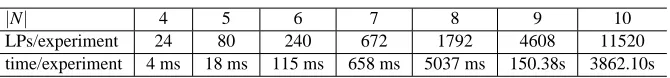
(N)|of LP problems to be tested for each experiment.

|N| 4 5 6 7 8 9 10

LPs/experiment 24 80 240 672 1792 4608 11520

time/experiment 4 ms 18 ms 115 ms 658 ms 5037 ms 150.38s 3862.10s

Table 5: The growth of computation times for|N|=4 to|N|=10.

5.2.1 RESULTS ANDDISCUSSION

Table 5 illustrates a natural increase in the time needed for one experiment as|N|increases. This is clear as both more LP problems have to be solved and they are of higher dimensions. For small values of|N|the increase in time occurs mainly because of the LP set up, not because of the com-putation itself. For higher|N|this proportion changes. But in spite of that, even for|N|=7 all 1000 experiments together could be done within minutes. For|N|=10 it took more than one month to perform all 1000 experiments; however, it took only about an hour for each single experiment. More specifically, on average, only about one third of a second was enough to test uL⇀ut for|N|=10.

Just looking at the increase of the dimensions of the LP problems, it is reasonable to assume that one can test independence implication for up to|N|=15 by directly plugging the corresponding LP problem into CPLEX. However, testing all|

E

(N)|inference problems for one experiment would be too expensive. Recall that one experiment already required about one hour of computation time for

|N|=10. To go even beyond|N|=15 for testing uL⇀ut, one can still exploit the known structure

of the matrix A of the LP problem and employ column generation techniques in order to solve these much bigger LP problems to optimality. Of course, this approach has to be coded and tested for bigger|N|to determine its efficiency.

6. Conclusions

Our computational experiments confirmed that the LP approach both overcomes the barriers of previous methods set by the number of variables in consideration and, moreover, it is also much faster. The new method also has the perspective to go even beyond the present limits, provided special LP techniques are used.

For small CI inference problems, involving a limited number of variables, one can enter data manually through web interfaces (based on LP method) available at

http://www.cs.waikato.ac.nz/˜remco/ci/.

For bigger inference problems, in which the input is expected in the form of a file, one can use efficient commercial LP software instead.

We showed that the potential application of computer testing of CI inference is in the area of Bayesian networks (see Section 2.4). More specifically, by Proposition 2 (and Corollary 3), testing independence inclusion (and reading CI restrictions from an acyclic directed graph) can be transformed to the task whether a difference of two standard imsets is a combinatorial imset. Since, by (3), every standard imset has at most 2· |N|non-zero values, and, also, its degree is at most

dare to conjecture that testing whether a difference of two standard imsets is a combinatorial imset can be done with polynomial complexity in|N|using the procedure from Section 4.2.1.

After finishing this paper, we learned about a conference paper by Niepert (2009), which also comes with the idea of application of the LP approach to probabilistic CI inference. The reader may be interested in what is the relation of both approaches. The LP problem in Niepert (2009, Proposition 4.9) is, in fact, equivalent to our task (9) with fixed factor k=1, if one uses a suitable one-to-one linear transformation to involved imsets u,v and w. This transformation has a nice

property that the transformed LP problem ˜Ax=˜b, x≥0has 0-1 matrix ˜A and ˜b≥0. However, since the transformation is linear and one-to-one, it is essentially the same LP problem. Our approach is more general because it allows one to consider the multiplicative factor k≥0 in (9), which results in a wider class of derivable CI implications (cf., Section 4.2.1). We hope that the algorithms presented in our paper will find their application, perhaps in the research on stable CI statements (Niepert, van Gucht, and Gyssens, 2010).

The results presented in the paper lead to further open theoretical problems. The most difficult one is probably to find out what is the exact value of the constant n∗ from Section 2.2 for|N|>5, as it seems to be related to finding the Hilbert basis

H

(N), which is a hard task. Another group of open questions concerns the verification of the implication u⇀v for u∈

C

(N)and v∈

E

(N). We would like to know the minimal bounds for the factors in (1), (6) and (8). Perhaps computing these bounds can be formulated as a mixed (integer) LP problem. Finally, there are general questions of complexity, like whether it is NP hard to decide CI implications with respect to the input size.

Acknowledgments

The research of Milan Studen´y has been supported by the grants GA ˇCR n. 201/08/0539 and M ˇSMT n. 1M0572. We thank the reviewers for their comments, which helped to improve the readability of the paper.

Appendix A. Proof of Proposition 1

Recall that L is an input list of CI statements over N and t another CI statement over N. The basic tool for our arguments is the multiinformation function mP:

P

(N)→Rascribed to any discrete

probability distribution P over N (for technical details see Studen´y, 2005, § 2.3.4). Corollary 2.2 in Studen´y (2005) says that mP is always a supermodular function and, for every CI statement s≡A⊥⊥B|C over N, one has

hmP,usi=0 iff A⊥⊥B|C[P]. (11)

Now, assuming uL⇀ut, the equivalent characterization (2) of the independence implication implies

that, for every discrete probability distribution P over N,

whenever hmP,uLi=0 then hmP,uti=0. (12)

Assuming P is a distribution such that every s in L is valid with respect to P, one hashmP,usi=0 by

(11), and, hence, by the linearity of the scalar product,hmP,uLi=∑s∈LhmP,usi=0. This implies,