A Heuristic Approach for Solving the Fixed Charge Transportation Problems

ISSN: 2306-9007 Altassan, El-Sherbiny, Ragab & Sasidhar (2018) 330

I

I

R

M

B

R

V

R

M

B

R

A Heuristic Approach for Solving the Fixed Charge

Transportation Problems

KHALID M. ALTASSAN

King Saud University, College of Business Administration, Saudi Arabia. Email: [email protected]

MAHMOUD M. EL-SHERBINY

King Saud University, College of Business Administration, Saudi Arabia Formerly at Institute of Statistical Studies and Research (ISSR), Cairo University, Egypt.

Email: [email protected]

ALY M. RAGAB

Institute of Statistical Studies and Research (ISSR), Cairo University, Giza, Egypt.

Email: [email protected]

BOKKASAM SASIDHAR

King Saud University, College of Business Administration, Saudi Arabia.

Email: [email protected]

Abstract

Most of researchers use the relaxed transportation problem proposed by (Balinski, 1961) to find approximate solution for the fixed charge transportation problem (FCTP). This approximated solution is considered as a lower limit for the optimal solution of FCTP. In this paper a heuristic approach has been developed to find an approximate solution used as a lower limit for the FCTP which is better than that is found by (Balinski, 1961). The same has been validated by applying the algorithm on 37 examples and testing for the significance of results. The algorithm is based on applying the Vogel approximation method on the relaxed transportation problem. In addition, an illustrative numerical example is given to show the simplicity of applying the proposed approach.

Keywords: Transportation Problem, Fixed Charge, Heuristic Methods.

Introduction

ISSN: 2306-9007 Altassan, El-Sherbiny, Ragab & Sasidhar (2018) 331

I

I

R

M

B

R

V

R

M

B

R

developed. Some of them are in (Adlakha & Kowalski, 2003; Adlakha, Kowalski, & Vemuganti, 2006; Cooper, 1975; Diaby, 1991; Gottlieb & Paulmann, 1998; Palekar, Karwan, & Zionts, 1990; Sun, Aronson, McKeown, & Drinka, 1998) .

An analytical branching method to solve the FCTP starting with a linear formulation of the problem that converges to an optimal solution by sequentially separating the fixed costs and finding a direction to improve the value of the objective function of the linear formulation has been proposed in (Adlakha, Kowalski, & Lev, 2010). An approximation for the lower bound of the FCTP is presented in (Adlakha, Kowalski, Wang, Lev, & Shen, 2014) and claimed that it is much superior to the lower bound developed in (Balinski, 1961). However, in the process, it was transformed to an NLP problem, which is computationally not simple.

The Fixed-charge Transportation Problem

The transportation model is a special case of the linear programming problem. It deals with transporting certain product from sources to destinations. The sources are production facilities with respictive

capacities and the destinations are warehouses with required levels of demands

The penality for transporting one unit of the given product from the source to the destination is . In the (FCTP) an additional fixed cost fij is assumed for opening the route (i, j) and the

problem is to determine the amounts to be transported from all sources to all destinations such that the total transportation cost is minimized while satisfying both the supply limits and the demand requirements.

The mathematical model of the FCTP can be represented as follows:

0 if 0 0 if 1 y 0 , (3) 1 for (2) 1 for s.t. ) 1 ( ) ( z ij 1 1 1 1              







Where xij is the unknown quantity to be transported through the route (i, j).

The Proposed Algorithm

This algorithm gives a better approximate solution for the FCTP that given in (Balinski, 1961). The proposed algorithm is an improved version of that Vogel Approximation Method (VAM) that generally produces a approximate solution for the traditional transportation problem. The basic idea of the algorithm is in adjusting the cost matrix of the Relaxed Transportation Problem (RTP), after each allocation (iteration) according to the changes in the supply and demand. The following steps illustrate the proposed algorithm:

Step1: Construct the Balinski RTP by relaxing the integer condition on yij (yij = fij/mij ) and the unit transportation cost Cij can be represented by (4).

)

4

(

/

ij

c

f

m

ISSN: 2306-9007 Altassan, El-Sherbiny, Ragab & Sasidhar (2018) 332

I

I

R

M

B

R

V

R

M

B

R

Where {

Step 2: For each row (column), determine a penalty by subtracting the smallest unit cost element in that row (column) from the next smallest unit cost element in the same row (column).

Step 3: Identify the row or column with the largest penalty. Break ties arbitrarily. Allocate as much as possible to the cell with the least cost in the identified row or column. Adjust the supply and demand, and cross out the satisfied row or column. If a row and a column are satisfied simultaneously, only one of the two is crossed out.

Step 4: If exactly one row (column) with positive supply (demand) remains uncrossed out, allocate this supply (demand) in the remaining uncrossed out cells with their unsatisfied demands (supply) of the uncrossed out column (row) and Stop. Otherwise go to step 5.

Step 5: Adjust the last cost matrix by recalculating the Cijfor the uncrossed out row (column) identified in

step 3. Go to step 3.

Numerical Example

Consider a company with four factories in locations S1, S2, S3 and S4 which produce a specific type of

product. There are six other locations D1, D2, D3, D4, D5 and D6 that receive this product as consumers. The

supply Si, the demand Dj, the cost fij for opening the route (i, j) and the unit cost cij for transporting one unit

of the given product from the source to the destination are given in Table 1.

Table1: Cost matrix fij, cij [13]

D1 D2 D3 D4 D5 D6 Supply

S1 11 , 0.69 16, 0.64 18, 0.71 17, 0.79 10, 1.7 20, 2.83 45

S2 14, 1.01 17, 0.75 17, 0.88 13, 0.59 15, 1.5 13, 2.63 35

S3 12, 1.05 13, 1.06 20, 1.08 17, 0.64 13, 1.22 15, 2.37 20

S4 16, 1.94 19, 1.5 15, 1.56 11, 1.22 15, 1.98 12, 1.98 15

Demand 35 30 25 15 5 5

Step 1: The Balinski RTP can be represented as in Table 2.

Table2: Balinski’s RTP matrix with Cij = cij + fij /mij

D1 D2 D3 D4 D5 D6 Supply

S1 1.00 1.17 1.43 1.92 3.70 6.83 45

S2 1.41 1.32 1.56 1.46 4.50 5.23 35

S3 1.65 1.71 2.08 1.77 3.82 5.37 20

S4 3.01 2.77 2.56 1.95 4.98 4.38 15

Demand 35 30 25 15 5 5

Step 2: Calculation of the penalty of each row (Pi) and of each column (Pj) is shown in Table 3.

Table 3: (Pi) and (Pj)

D1 D2 D3 D4 D5 D6 Supply Pi

S1 1.00 1.17 1.43 1.92 3.70 6.83 45 0.17

S2 1.41 1.32 1.56 1.46 4.50 5.23 35 0.09

S3 1.65 1.71 2.08 1.77 3.82 5.37 20 0.06

S4 3.01 2.77 2.56 1.95 4.98 4.38 15 0.61

Demand 35 30 25 15 5 5

ISSN: 2306-9007 Altassan, El-Sherbiny, Ragab & Sasidhar (2018) 333

I

I

R

M

B

R

V

R

M

B

R

Step 3: From Table 3, the sixth column has the maximum penalty (0.85) and the minimum cost in this column is 4.38 in the cell (4, 6). So, the cell (4, 6) is allocated with the maximum possible value (5 units) which is the minimum of S4 and D6. Cross out the column D6 corresponding to this minimum.

The uncrossed out row is the fourth row, then change the supply S4 to 10. The result of this step is

allocating 5 units in the cell (4, 6). This means that x46 = 5.

Step 4: Since there are more than one row (column) with positive supply (demand) uncrossed out, go to step 5.

Step 5: Since the uncrossed out row in step 3 is S4, calculate the costs C4j for row S4 based on its new

supply (10). The new cost matrix is presented in Table 4. Note that the costs in row S4 only are

changed due to changing S4 from 15 to 10. Go to step 3.

Table 4: Cost Matrix from Step 4

D1 D2 D3 D4 D5 Supply Pi

S1 1.00 1.17 1.43 1.92 3.70 45 0.17

S2 1.41 1.32 1.56 1.46 4.50 35 0.09

S3 1.65 1.71 2.08 1.77 3.82 20 0.06

S4 3.54 3.40 3.06 2.32 4.98 10 0.74

Demand 35 30 25 15 5

Pj 0.41 0.14 0.13 0.32 0.12

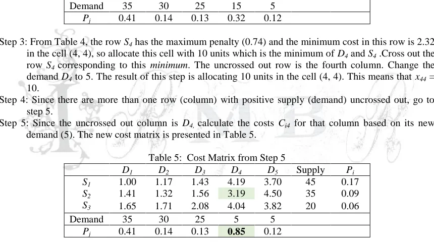
Step 3: From Table 4, the row S4 has the maximum penalty (0.74) and the minimum cost in this row is 2.32

in the cell (4, 4), so allocate this cell with 10 units which is the minimum of D4 and S4 .Cross out the

row S4 corresponding to this minimum. The uncrossed out row is the fourth column. Change the

demand D4 to 5. The result of this step is allocating 10 units in the cell (4, 4). This means that x44 =

10.

Step 4: Since there are more than one row (column) with positive supply (demand) uncrossed out, go to step 5.

Step 5: Since the uncrossed out column is D4, calculate the costs Ci4 for that column based on its new

demand (5). The new cost matrix is presented in Table 5.

Table 5: Cost Matrix from Step 5

D1 D2 D3 D4 D5 Supply Pi

S1 1.00 1.17 1.43 4.19 3.70 45 0.17

S2 1.41 1.32 1.56 3.19 4.50 35 0.09

S3 1.65 1.71 2.08 4.04 3.82 20 0.06

Demand 35 30 25 5 5

Pj 0.41 0.14 0.13 0.85 0.12

Step 3: The result of this step is transporting 5 units through the route (2, 4). That means x24 = 5.

Step 4: Since there are more than one row (column) with positive supply (demand) uncrossed out, go to step 5.

Step 5: Since the uncrossed out row is S2, recalculate the cost C2j. The result of this step is presented in

Table 6.

Table 6: Recalculated costs of Step 5

D1 D2 D3 D5 Supply Pi

S1 1.00 1.17 1.43 3.7 45 0.17

S2 1.48 1.32 1.56 4.5 30 0.09

S3 1.65 1.71 2.08 3.82 20 0.06

Demand 35 30 25 5

ISSN: 2306-9007 Altassan, El-Sherbiny, Ragab & Sasidhar (2018) 334

I

I

R

M

B

R

V

R

M

B

R

Step 3: The result of this step is transporting 35 units through the route (1, 1). That means x11 = 35, the S1

would be equal to 10 and the crossed out column D1.

Step 4: Since there are more than one row (column) with positive supply (demand) uncrossed out, go to step 5.

Step 5: Since the uncrossed out row is S1, recalculate the cost C1j as presented in Table 7.

Table 7: Recalculated costs of Step 5

D2 D3 D5 Supply Pi

S1 2.24 2.51 3.7 10 0.27

S2 1.32 1.56 4.5 30 0.24

S3 1.71 2.08 3.82 20 0.37

Demand 30 25 5

Pj 0.39 0.52 0.12

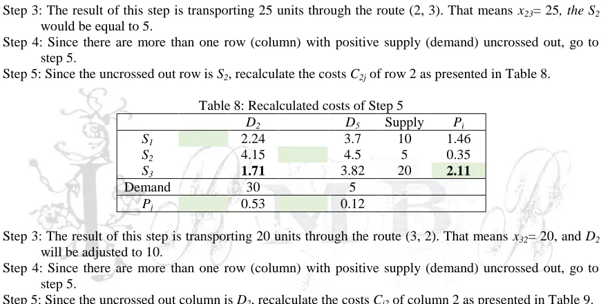
Step 3: The result of this step is transporting 25 units through the route (2, 3). That means x23= 25, the S2

would be equal to 5.

Step 4: Since there are more than one row (column) with positive supply (demand) uncrossed out, go to step 5.

Step 5: Since the uncrossed out row is S2, recalculate the costs C2j of row 2 as presented in Table 8.

Table 8: Recalculated costs of Step 5

D2 D5 Supply Pi

S1 2.24 3.7 10 1.46

S2 4.15 4.5 5 0.35

S3 1.71 3.82 20 2.11

Demand 30 5

Pj 0.53 0.12

Step 3: The result of this step is transporting 20 units through the route (3, 2). That means x32= 20, and D2

will be adjusted to 10.

Step 4: Since there are more than one row (column) with positive supply (demand) uncrossed out, go to step 5.

Step 5: Since the uncrossed out column is D2, recalculate the costs Ci2 of column 2 as presented in Table 9.

Table 9: Recalculated costs of Step 5

D2 D5 Supply Pi

S1 2.24 3.7 10 1.46

S2 4.15 4.5 5 0.35

Demand 10 5

Pj 1.91 0.80

Step 3: The result of this step is transporting 10 units through the route (1, 2). Cross out D2 and adjust S1to 0 as in Table 10.

Table 10: Recalculated costs of Step 5

D2 D5 Supply Pi

S1 3.7 0 1.46

S2 4.5 5 0.35

Demand 5

ISSN: 2306-9007 Altassan, El-Sherbiny, Ragab & Sasidhar (2018) 335

I

I

R

M

B

R

V

R

M

B

R

Step 4: Since there is only one column (D5) with positive demand (5) uncrossed out, allocate 5 units to the

cell (2, 5) and stop. The final allocation is shown in Table 11.

Table 11: Final allocation

D1 D2 D3 D4 D5 D6 Supply

S1 35 10 0 45

S2 25 5 5 35

S3 20 20

S4 10 5 15

Demand 35 30 25 15 5 5

The total variable cost



 

m

i n

j ij ij

x

c

of final allocation is 106.3, the total fixed cost



 

m

i n

j ij ij

y

f

is 108 and

the total cost

(

)

1 1

ij ij m

i n

j ij ij

x

f

y

c





 

is 214.3. While the proposed algorithm finds an initial feasible solution

with total cost equals 214.3, which is less than the initial feasible solution (the optimal RTP solution) given in (Balinski, 1961) gives total cost of 229.1.

Computational Results and Analysis

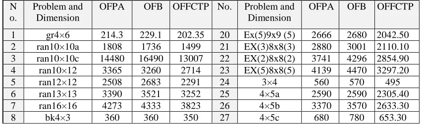
As many as 37 FCTP problems have been chosen, with different dimensions (ranging from 3x4 up to 17×17) from different references, including from OR library ("OR Library: Testcases for Transportation Problems, Fixed Charge Transportation Benchmark Problems,,") and (Adlakha et al., 2014). Table 12

shows a comparison between the objective functions of the approximate solutions using the proposed

algorithm (OFPA) and the results of the approach (OFB) proposed in (Balinski, 1961), who adopted results from (Adlakha et al., 2010). The two approaches gave the same solutions for 7 problems viz., 8, 25, 26, 28, 29, 31 and 32. The approach gave better solutions for 4 problems viz., 9, 17, 35 and 36. In order to establish how close is the objective function of the approximate solution to the optimal solution of the FCTP (OFFCTP), using both the proposed algorithm and the approach in (Balinski, 1961), paired-sample t-test was carried out. The test was carried out on the results of 37 problems considered in Table 12. The results of the test are presented in Tables 13 and 14. It can be observed that the difference between the value of the objective function of the approximate solution by the proposed algorithm and the optimal solution of the FCTP is significantly lower than the difference between the proposed and value of the objective function of the approximate solution by the Balinski’s approach (Balinski, 1961) and the optimal solution of the FCTP. Hence the proposed algorithm can be considered superior to that of Balinski’s and provides a technique for finding the initial solution for the FCTP.

Table 12: Comparison between the objective functions of approximate solutions using the proposed algorithm and the Balinski’s approach.

N o.

Problem and Dimension

OFPA OFB OFFCTP No. Problem and

Dimension

OFPA OFB OFFCTP

1 gr4×6 214.3 229.1 202.35 20 Ex(5)9x9 (5) 2666 2680 2042.50

2 ran10×10a 1808 1736 1499 21 EX(3)8x8(3) 2880 3001 2110.10

3 ran10×10c 14480 16490 13007 22 EX(2)8x8(2) 3741 4296 2854.90

4 ran10×12 3365 3260 2714 23 EX(5)8x8(5) 4139 4470 3297.20

5 ran12×12 2508 2683 2291 24 3×4 560 570 495

6 ran13×13 3390 3521 3252 25 4×5a 2590 2590 2305.40

7 ran16×16 4273 4333 3823 26 4×5b 3370 3570 2633.30

ISSN: 2306-9007 Altassan, El-Sherbiny, Ragab & Sasidhar (2018) 336

I

I

R

M

B

R

V

R

M

B

R

9 ran17×17 1525 1464 1373 28 4×5d 9900 9900 8946.70

10 bal8×12 501 504.2 471.5 29 4×5e 1960 1960 1743.30

11 kow4×5 265 285 250 30 4×5f 315 320 305.80

12 Kawl4×5 335 345 335 31 4×5h 325 325 296.70

13 ran10×10bT 3491 3546 2672.80 32 4×5i 345 345 311.70

14 ran10×10cT 16591 16653 12544.7 33 3×4 30350 30455 29950

15 ran10×12T 2874 3289 2326.70 34 4×5 395 405 325.70

16 ran12×12T 2559 2691 1972.30 35 4×6 835 805 740

17 Ex(3)7x8 2545 2449 1970.60 36 4×5 3170 3150 2620.00

18 Ex(15)7x8(3) 2493 2510 1974.20 37 4×5 1350 1360 1350.00

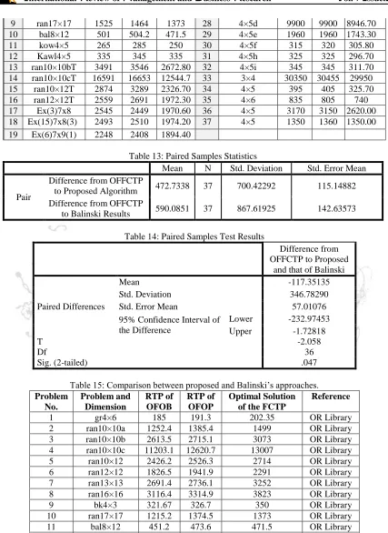
19 Ex(6)7x9(1) 2248 2408 1894.40

Table 13: Paired Samples Statistics

Mean N Std. Deviation Std. Error Mean

Pair

Difference from OFFCTP

to Proposed Algorithm 472.7338 37 700.42292 115.14882

Difference from OFFCTP

to Balinski Results 590.0851 37 867.61925 142.63573

Table 14: Paired Samples Test Results

Difference from OFFCTP to Proposed

and that of Balinski

Paired Differences

Mean -117.35135

Std. Deviation 346.78290

Std. Error Mean 57.01076

95% Confidence Interval of the Difference

Lower -232.97453

Upper -1.72818

T -2.058

Df 36

Sig. (2-tailed) .047

Table 15: Comparison between proposed and Balinski’s approaches. Problem

No.

Problem and Dimension

RTP of OFOB

RTP of OFOP

Optimal Solution of the FCTP

Reference

1 gr4×6 185 191.3 202.35 OR Library

2 ran10×10a 1252.4 1385.4 1499 OR Library

3 ran10×10b 2613.5 2715.1 3073 OR Library

4 ran10×10c 11203.1 12620.7 13007 OR Library

5 ran10×12 2426.2 2526.3 2714 OR Library

6 ran12×12 1826.5 1941.9 2291 OR Library

7 ran13×13 2691.4 2736.1 3252 OR Library

8 ran16×16 3116.4 3314.9 3823 OR Library

9 bk4×3 76.1:; 326.7 350 OR Library

10 ran17×17 1215.2 1374.5 1373 OR Library

11 bal8×12 89.16 473.6 471.5 OR Library

12 ran14×18 3016.9 3227.5 3712 OR Library

13 kow4×5 226 258.3 250 Adalkha

ISSN: 2306-9007 Altassan, El-Sherbiny, Ragab & Sasidhar (2018) 337

I

I

R

M

B

R

V

R

M

B

R

Table 15 shows that the values of the RTP obtained by the proposed approach (OFOP) lies between the values of the RTP given by Balinski’s approach (OFOB)(Balinski, 1961) and the optimal solution of the RTP matrix, for some of the problems considered in OR library ("OR Library: Testcases for Transportation Problems, Fixed Charge Transportation Benchmark Problems,,") and (Adlakha et al., 2014). Also, all the values do not penetrate the optimal values of such problems. Hence, the RTP values given by the proposed algorithm can be considered as a lower bound – as a reference - for the optimal solution of FCTP instead of using the RTP value given by the optimal solution of RTP matrix as mentioned in (Adlakha et al., 2010).

Conclusion

This paper presented a heuristic approach for finding an approximate solution used as a lower bound for the optimal solution of FCTP. This heuristic approach has been applied to a set of problems and the results indicate that it is significantly better. The RTP value using this algorithm can be considered as a better lower bound to the optimal solution of FCTP compared to the RTP value obtained by Baliniski’s approach (Balinski, 1961). In addition, the proposed algorithm is simple and computationally feasible as compared to the algorithm presented in (Adlakha et al., 2014) which is dealing with a non-linear formulation of the problem.

Acknowledgement

This paper is supported by the Research Center at the College of Business Administration and the Deanship of Scientific Research at King Saud University, Riyadh.

References

Adlakha, V., & Kowalski, K. (2003). A simple heuristic for solving small fixed-charge transportation

problems. Omega, 31(3), 205-211.

Adlakha, V., Kowalski, K., & Lev, B. (2010). A branching method for the fixed charge transportation

problem. Omega, 38(5), 393-397.

Adlakha, V., Kowalski, K., & Vemuganti, R. (2006). Heuristic algorithms for the fixed-charge

transportation problem. Opsearch, 43(2), 132-151.

Adlakha, V., Kowalski, K., Wang, S., Lev, B., & Shen, W. (2014). On approximation of the fixed charge transportation problem. Omega, 43, 64-70.

Altassan, K. M., El-Sherbiny, M. M., & Sasidhar, B. (2013). Near Optimal Solution for the Step Fixed

Charge Transportation Problem. Applied Mathematics & Information Sciences, 7(2), 661-669.

Balinski, M. (1961). Fixed cost transportation problems. Naval Research Logistics Quarterly, 8, 41–54.

Cooper, L. (1975). The fixed charge problem—I: a new heuristic method. Computers & Mathematics with

Applications, 1(1), 89-95.

Diaby, M. (1991). Successive linear approximation procedure for generalized fixed-charge transportation

problems. Journal of the Operational Research Society, 42(11), 991-1001.

Gottlieb, J., & Paulmann, L. (1998). Genetic algorithms for the fixed charge transportation problem. Paper presented at the Evolutionary Computation Proceedings, 1998. IEEE World Congress on Computational Intelligence., The 1998 IEEE International Conference on.

Hirsch, W. M., & Dantzig, G. B. (1954). Notes on Linear Programming, Part XIX: The Fixed Charge Problem: Rand Corporation.

OR Library: Testcases for Transportation Problems, Fixed Charge Transportation Benchmark Problems,. Palekar, U. S., Karwan, M. H., & Zionts, S. (1990). A branch-and-bound method for the fixed charge

transportation problem. Management Science, 36(9), 1092-1105.

Sun, M., Aronson, J. E., McKeown, P. G., & Drinka, D. (1998). A tabu search heuristic procedure for the