Improving Activated Sludge Wastewater Treatment Process Efficiency Using Predictive Control

Improving Activated Sludge Wastewater Treatment Process Efficiency

Using Predictive Control

Ioana Nascu

,

Ioan Nascu

1

Artie McFerrin Department of Chemical Engineering, Texas A&M, College Station TX, USA.

2

Department of Automation, Technical University of Cluj-Napoca, Romania.

Received 05, June 2017; received in revised form 07, June 2017; accepted 09, July 2017

Abstract

This paper investigates the performance of a new predict ive control approach used to improve the energy

efficiency and effluent quality of a conventional Wastewater Treatment Plant (WWTP). A modified variant of the

well-known Generalized Predictive Control (GPC) method has been applied to control the dissolved oxygen

concentration in the aerobic bioreactor of a WWTP. The quadratic cost function was modified to a positional

imple mentation that considers control signal weighting and not its increments, in ord er to minimize the control

energy. The Activated Sludge Process (ASP) optimizat ion using the proposed variant of the GPC a lgorith m provides

an improved aeration system effic iency to reduce energy costs. The control strategy is investigated and evaluated by

performing simulations and analyzing the results. Both the set point tracking and the regulatory performances have

been tested. Moreover, the effects of some tuning parameters are also investigated. The results show that this control

strategy can be efficiently used for dissolved oxygen control in WWTP.

Keywords: predict ive control, process optimization, process model, wastewater treat ment plant, activated sludge treatment

1.

Introduction

Wastewater treatment plants are key infrastructures for ensuring a proper protection of our environment. Biologica l

treatment is an important and integral part of any WWTP. The Activated Sludge Process is the most commonly used

technology to treat sewage and industrial wastewaters due to its flexibility, high reliability and cost-effectiveness, as well as its

capacity of producing high quality effluent. An overv iew of the activated sludge wastewater treat ment process mathemat ical

modeling is presented in [1] and application of ASP models can be found in [2]. The ASPs a re d ifficult to be controlled because

of their co mple x and nonlinear behavior. However, the optima l control of the biologica l reactors plays an important role in t he

operation of a WWTP and the efficiency of most WWTP is an important issue still to be improved .

A good control of WWTP processes could lead to better water quality and t o an effic ient use of energy [3-4]. This research

area is a key part of keeping the environ ment clean and nowadays has received great emphasis due to the strict regulations fo r

the discharged water. Many o f the WWTP are operated in a less -than-optimal manner with respect to both treatment and

energy efficiency, causing high costs and inefficient operation in order to meet the regulations.

*Corresponding author. E-mail address: [email protected]

The dissolved oxygen concentration has a ma jor impact in the activated sludge process. To control the dissolved oxygen

concentration, the a mount of air provided by the blowe rs in the ae ration tank is modified. The activated sludge process is the

most energy consuming process es in the whole WWTP, nearly half of the energy consumed in a WWTP being used in the

aeration tank. An over dosage of aeration is unwanted because it brings increased costs and just little or even no gain in the

quality of water. Fo r values of dissolved oxygen concentration in the aeration tank above 2 mg/l, the increase of the aeration

flow begins to have a lower effect in the quality of effluent and at values of 4-6 mg/ l doesn’t have any effect. In the absence of

adequate control systems, to reduce the effect o f disturbances on the flow or load of the effluent, it is sometimes preferred to

operate at high concentrations of dissolved oxygen in the aerat ion tank. Using the blowe rs in manual operation at constant flow

rates during the periods of reduced wastewater intake will produce a loss of energy. Thus, optimizing the aerat ion process

defines an important objective to reduce energy consumption and imp rove energy effic iency. Severa l strategies have been

proposed for controlling the dissolved oxygen concentration. So me researchers have focused on the importance of we ll -tuned

models and simu lation p latforms in the process of designing the controllers for the dissolved oxygen concentration [5-6]. Other

researchers have focused on designing multip le model controllers instead of nonlinear comp le x ones [7]. Nevertheless,

because of the high nonlinearit ies of the process, robust controllers are required to maintain an optimu m setpoint, regardles s of

the changes in the operating point. Such control strategies have also been proposed, including adaptive [8-9], predict ive

[10-11], fuzzy [12] or fractional order PIμDλ control [13].

Optimizing and ma intaining the dissolved oxygen set point define important objectives for researchers in WWTP c ontrol.

Optimization of the dissolved oxygen set point is not the purpose of this paper. In practice, an appropriate dissolved oxygen set

point is determined either manually by e xperienced operators or automatica lly through optimization algorith ms. In this paper,

we assume the appropriate set point is prescribed by the optimizing part of a mult ilayer hie rarchica l control structure and the

proposed control system will be responsible for forcing the plant to follow this set -point. A modified variant of the well-known

Generalized Predict ive Control method [14] has been applied to control the d issolved oxygen concentration in the aeration tank

of an activated sludge process . The ASP process optimization using the proposed variant of the GPC a lgorith m provides an

improved aeration system effic iency to reduce energy costs. The GPC a lgorith m is well known and consists of applying a

control sequence that minimizes a quadratic cost function defined over a prediction horizon. The consideration of weighting o f

control incre ments in the cost function in GPC allows an incre mental imp le mentation which ensures offset-free re ference

tracking and disturbance rejection but does not provide minimizat ion of the control energy. To a lleviate the above mentioned

limitat ion, the aim of this paper is to propose a different variant of the quadratic cost function. In order to minimize the control

energy, the quadratic cost function was modified to a positional imp le mentation that considers control signal weighting and n ot

its incre ments. To evaluate the performance of the proposed design for ASP process optimizat ion, simulat ion results are

presented and discussed in detail. The ASP process was first modeled and the models were calibrated and validated based on a

combination of laboratory tests and plant operating measured data. The proposed control strategy is investigated and evaluated

by performing simulations and analyzing the results. Both the set poin t tracking and the regulatory performances have been

tested. Moreover, the effects of some tuning parameters are also investigated. The results show that this control strategy ca n be

efficiently used for dissolved oxygen control in WWTP.

2.

Process Description and Modeling

The activated sludge wastewater treatment processes are very co mple x, with large, uncontrollable input disturbances,

significant nonlinearities and characterized by uncertainties regarding their para meters. The most widely used models to

describe these processes is the Activated Sludge Model Nr.1 (ASM 1) proposed by the International Water Association (IWA)

the behavior of the process. Since the model a lso contains a large number of b iokinetic and stoichiometries parameters, for

control purposes it is necessary to simplify it into a simpler model, especially if a hierarchical control structure is used.

The modelling process and the model ca libration are made based on data obtained from a conventional activated sludge

system operating under aerobic conditions and whose main purpose is to ensure the removal o f colloida l and dissolved

carbonaceous organic matter. The res idual water that needs to be treated is coming fro m a factory that processes and is painted

cotton, a milk factory and from domestic households.

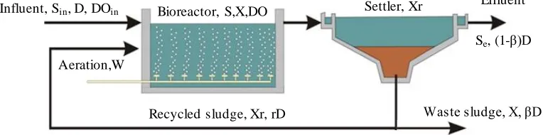
Fig. 1. WWTP's biological treatment process schematic configuration.

The wastewater first enters the aerated bioreactor where the treatment based on ASP takes place. The clea r water and the

sludge are separated due to gravity in the secondary settler. In orde r to keep b iological sustainability, the act ive sludge is

recirculated and the bioreactor is aerated using an aeration network where air is being blown with fine bubbles.

In our previous work [16-17] we have developed a reduced model to the ASP based wastewater treatment process where the simplest possible case was taken into consideration. Only the re moval of organic matter is considered, while bio logical

phosphorus and nitrogen re moval is neglected . The following co mponents are treated in the model: one organic matter

component, one microorganism co mponent and dissolved o xygen. For the model used in this paper, t wo processes are

considered to take place in the aeration tank: the reduction of organic substance in heterotrophic aerobic bacteria and the

reduction of ammonia n itrogen with autotrophic aerobic bacteria. The carbonaceous conversion is integrated in a consistent

manner with the transformations of nitrogen. The following components are treat ed in the model: one organic matter

component, two nitrogen components, two microorganism components and dissolved oxygen.

The developed model is based on the following assumptions: the content of the aeration tank is considered perfect stirred;

there are no d irections in the secondary settler; the bio mass concentration in the e ffluent is negligible; the o xygen concentration

and substrate are neglected in the recycled sludge; the active sludge is the only recycled component into the aeration tank.

In this case, there are 6 equations. that can be written for the aeration tank considered as a completely mixed reactor. Eqs.

(1-6) correspond to the mass balance Eqs. for:heterotrophic (1) and autotrophic (2) b io mass, biodegradable substrate (3),

ammonia nitrogen (4), nitrite and nitrate nitrogen (5) and dissolved oxygen(6) concentration.

( )

( ) ( ) ( )(1 ) ( ) [ ( ) ( ) ] ( )

B,H

r B,H B,H H Ha H B,H

dX t

= r D t X t D t + r X t + m t + m t b X t

dt     (1)

( )

( ) ( ) ( )(1 ) ( ) [ ( ) ] ( ) B,A

r B,A B,A A A B,A

dX t

= r D t X t D t + r X t + m t b X t

dt    (2)

( ) ( ) ( )

( ) ( )[( ) ( ) ( )]

S H Ha

B,H S Sin

H

dS t m t + m t

= X t D t 1+ r S t + S t

dt  Y  (3)

Bioreactor, S,X,DO Settler, Xr

Recycled sludge, Xr, rD Waste sludge, X, βD Aeration,W

Influent, Sin, D, DOin

Effluent

, ,

( ) 1 1

= ( ) ( ) ( ) ( ) ( )[(1 ) ( ) ( )] 2.86

NO

Ha B H A B A NO NOin

H A

dS t YH

m t X t m t X t D t r S t S t

dt Y Y



     (4)

( ) 1

[ ( ) ( )] ( ) ( ) ( ) ( ) ( )[(1 ) ( ) ( )] NH

XB H Ha BH XB A BA NH NHin

A

dS t

= -i m t + m t X t - i + m t X t - D t + r S t + S t

dt Y (5)

1 ( )

( ) ( ) (1 ) ( ) ( ) ( )[(1 ) ( ) ( )] [ ( )] H

in max

H B,H A B,A

H A

Y

dDO t 4.57

= m t X t m t X t D t +r DO t + DO t ++aW DO DO t

dt Y Y



     (6)

The mass balance equations for the recycled biomass are:

) ( ) )( ( ) ( ) 1 )( ( ) ( , , , t X r t D t X r t D dt t dX H rB S H B S H

rB _{    (7)}

,

, ,

( )

( )(1 ) ( ) ( )( ) ( )

rB A

S B A S rB A

dX t

D t r X t D t r X t

dt     (8)

Under steady state conditions, from mass balance equations in the settling tank the resulting concentrations in the effluent SSef,

SNHef and SNOef are:

( )

(1

)

( )

Sef S

S

t =

+ r S t

( ) (1 ) ( )

NHef NH

S t = +r S t (10)

(t) S r) + (1 (t)

SNOef  NO (11)

The equations for the heterotrophic growth of the biomass in aerobic (µH) and anoxic (µHa) conditions are:

H Hmax , ( ) ( ) ( ) ( ) ( ) S

S S O H

S t DO t

t

K S t K DO t

  

  (12)

H a Hmax

,

( ) ( )

( )

( ) ( ) ( )

S OH NO

g

S S O H NO NO

S t K S t

t

K S t K DO t K S t

    

   (13)

While the equation for the growth of autotrophic mass µA is:

) ( ) ( ) ( ) ( (t) , Hmax A t DO K t DO t S K t S A O NH NH NH    

 ₍₁₄₎

where XB,H and XB,A represent the active heterotrophic and autotrophic biomass concentration, SS, SNH, SNO, and DO -

concentration of b iodegradable organic matter, a mmonia nitrogen, n itrite -n itrate, and dissolved oxygen in the aerated

bioreactor, SSin, SNHin, and SNOin - concentrations in the influent, XrB,H and XrB,A - recycled heterotrophic and autotrophic bio mass

concentrations, D and DS - dilution rates (ratio of influent flow to volu me of the aerated bioreactor and settler), W - aeration rate,

α - o xygen transfer rate, r - the ratio of recycled sludge flo w to influent flow, β - the ratio of waste flow to influent flow, YA -

autotrophic biomass yield factor, YH - heterotrophic bio mass yield factor, iXB - conversion coefficient for the nitrogen mass,

KOH and KOA - oxygen saturation coefficients at half for heterotrophic/autotrophic biomass, KNH and KNO - ammonia and nitrate

saturation coeffic ients at half for autotrophic bio mass, KS - organic substrate saturation coefficient, ηg - correct ion coeffic ient

for µH in ano xic conditions. This model has 8 state variables: XB,H, XB,A, XrB,H, XrB,A, SS, SNH, SNO, and DO. The kinetic and

stoichiometric para meters va lues obtained after the model calibrat ion are : bH=0.034; bA=0.002; YH=0.54; YA=0.13; iXB=0.068; α

3.

Control Strategy

The aeration system, the b lower and p iping model and th e proportional–integral–derivative (PID) control of the air flow is

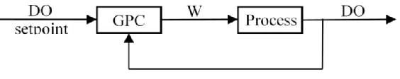
presented in [18-19]. Following this work, this paper investigates the performance of a mod ified variant of the we ll-known

Generalized Pred ictive Control (GPC) method to control the dissolved oxygen concentration (DO) in the aerated bioreactor of

an activated sludge process , considered as process output variable (Fig. 2). We assume that the appropriate set point for the

dissolved o xygen concentration is given and the predict ive control system is used to maintain this set point. The aeration a ir

flow (W) is considered as manipulated variable.

Fig. 2 Predictive control schemes

The Generalized Predictive Controller is one of the most relevant design methods of Model-Based Pred ictive Control

(MBPC). The standard GPC synthesis is based on a linear p rocess model, CARIMA - Controlled Auto-Regressive Integrated

Moving-Average, a quadratic cost function and a control law, both using an incremental structure (the actual control signal

incre ment - Δu- is co mputed) [14]. Th is incre mental imple mentation ensures offset -free behavior in closed loop control

systems.

The activated sludge process is the most energy consuming process es in the whole WWTP, nearly half of the energy

consumed in a WWTP being used for the aeration. An important step in developing the proposed control strategy is the

repara metrizat ion of the cost function in the pred ictive a lgorith m to contain a measure of energy consumed by ae ration process.

This could exploit the fluctuation of operating conditions by realizing significant energy savings. Since the aeration air flow W

is the manipulated variable resulted fro m the con troller output u, to minimize the aeration flow and not its variations the repara metrized cost function of the predictive algorithm has to contain the controller output u, instead of the control output incre ment Δu. This will lead to a positional imp le mentation based on a positional form for the process model and controller

cost function.

Consider the following modified MBPC cost function:

2

1

2 2

1 2

1

( , , ) [ ( ) ( )] [ [ ( 1)]

u

N N

u r

j N j

J N N N E y t j y t j



 

 

 

 _       _

 







where: y r is the future refe rence sequence, N1 is the minimu m costing horizon, N2 is the ma ximu m costing horizon, Nu is the

control horizon,and ρ is a control-weighting coefficient

.

The use of the CARMA process model instead of the CARIMA model :

1 1 1

( ) ( ) ( ) ( ) ( ) ( )

A q y t B q u t k C q e t (16)

will lead to a positional form for the controller and therefore the controller will not have an integrator.

1 1 1

1E q_j( ) (A q)q F qj _j( ) (17)

where Ej(q-1) and Fj(q-1) are polynomia ls uniquely defined, given A(q-1) and the prediction interval j, o f degree j and

respectively n (n - the process order).

Based on Eq. (16) and Eq. (17) we obtain:

1 1 1 1

( ) j( ) ( ) ( ) j( ) ( ) j( ) ( )

y t j E q B q u t   j k F q y t E q e t j (18)

The optimal predictor, given measured data up to time t (including t) is written as:

1 1 1

( | ) j( ) ( ) j( ) ( ) j( ) ( )

y tj t G q u t  j k F q y t E q e tj (19)

where

) ( ) ( )

( 1 _ 1 _ 1

q B q E q

Gj j (20)

For simplic ity, in the derivation below, N1 is set to 1, N2 to N, Nu to N and k to 1. For j = 1,...,N,the optima l predictor Eq. (18)

can be written::

1

0 1 0 1

( ) ( ) [ ( ) ] ( ) ( ) ( 1) ( )

1

y t 1 g u t  G q g u t F y t E q e t1 (21)

1 1 1

1 0 2 1 0 2

( ) ( ) ( ) [ ( ) ] ( 1) ( ) ( ) ( 1) ( )

2

y t2 g u t g u t    1 G q q g g u t F q y t E q e t2 (22)

1 ( 1)

1 0

1

( ) ( ) ( ) [ ( ) ... ] ( 1)

( ) ( ) ( ) ( )

N

N -1 0 N N

1

N N

y t N g u t ... g u t N 1 G q q g g u t N

F q y t E q e t N

   

 

             

   (23)

On observe that the predictor y (t+j), consists of three terms: one including the past known control actions and the filtered

measured process outputs, the second depending on future control actions which must be determined and the third, depending

on the future noise signals. Let f( t+j) be the component of y (t+j), which includes all the known terms at a timely moment:

1

1 0 1

1 ( ) ( )

f(t ) [G (q )g ]u t F y t ₍₂₄₎

1 1 1

2 1 0 2

( 2) [ ( ) ] ( 1) ( ) ( )

f t  G q q g g u t F q y t (25)

1 ( 1)

1 0

(

) [

(

)

...

] (

1)

(

) ( )

f t



N



G q



q

g

 

g u t

  

N

F q

y t

Then Eq. (19) can be rewritten in the vectorial form:

e f u G

y    (27)

where y, u, f and e are vectors of the form: [ ( 1), ..., ( )] , x 1T

y y t y t N N (28)

[ ( ), ..., ( 1)] , x 1T

u u t u t N  N (29)

[ ( 1), ..., ( )] , x 1T

f  f t f t N N (30)

1 1

1

[ ( ) ( 1), ...,

e E q e t E q e tN N (31)



































1 N 2 N 3 0

N 0 1 2 0 1 0

g

...

g

g

g

...

...

...

...

...

0

...

g

g

g

0

...

0

g

g

0

...

0

0

g

G

For N u < N the matrix G is then of dimension N x N u:

                   

 g g ... gN Nu g ... ... ... ... ... 0 ... g g g 0 ... 0 g g 0 ... 0 0 g G 3 N 2 N 1 N 0 1 2 0 1 0 (33)

And y, u, f and e are vectors of the form: [ ( 1), ..., ( )] , x1T

y y t y tN N (34)

[ ( ), ..., (

1)] ,

x1

u



u t

u t N





N

[ (

1), ..., (

)] , x1

f



f t



f t N



N

1 1

1

[ ( ) ( 1), ...,

e E q e t E q e tN N (37)

The cost function becomes:

( ) [( )T( ) T ] [( )T( ) T ]

u r r r r

J 1,N,N = E y -y y -y + uu = E Gu+ f +e -y Gu+ F +e -y +uu (38)

Assuming that E[eTu]=0, E[e]=0, and E[eTe] is not affected by u, the first derivative of the previous equation gives:

[ T( ) ] [( T ) T( )]

r r

J

= 2EG Gu + f +e -y + Iu = 2E GG+ I u +G f -y

u  



 (39)

For the first derivatal ive equate zero the control vector u is obtained:

1

( T ) T( )

r

u G GI G y f (40)

Only the first element of u vector, u(t), must be determined and this value represents the current controller output:

) ( )

(t y f

u r

T _





where α T _{= [α}

1... αN] is the first row of the (G TG+ρI) -1G T matrix. Note that if the equation for the calculation of the controller

output (u) has the same form as that for the incremental GPC a lgorith m (Δu), the diophantine equation form and calculat ion of

polynomials Ej and Gj is different.

4.

Simulation Results

The assessment of the developed control system is done through numerica l simulation in Matlab/SIM ULINK

environment. The nonlinear model of the activated sludge wastewater treatment process given by Eqs. (1)-(14) was used to

simu late the process dynamics. In the GPC a lgorith m the pred iction of the process output is based on a linear process model.

To obtain the linear state space model and the transfer function fro m W to DO the model was linearized a roun d an operating

state-space realizat ion was first computed and then the smallest 6 diagonal entries of the balanced grammians were e liminated

using modred. Simila r results were obtained using the input and output data obtained during simulat ions of the nonlinear model

dynamics for sma ll variations around the considered operating point and a Recursive Least Square algorithm to estimate a

second order discrete transfer function.

The steady state values of the input variables are: DO=0.064[h-1]; DOin0=0.5[mg/l]; Sin0=765[mg/l]; W0=100[m3/h] and

r0=0.8. The steady state value for the considered process output is DO0 =1.36 mg/ l. The aeration air flo w (W) is considered as

the manipulated input, the other inputs being considered as disturbances. The air flow values were limited between Wmin =

50m3/h and Wmax =210m3/h. The controller design para meters are : N=6, Nu=1, sa mpling period ts= 0.01 h. Diffe rent aspects,

such as setpoint changes and effects of load disturbances , have been analyzed.

In Fig. 3 the setpoint tracking for a step fro m DO0 =1.36 mg/l to DO1 = 2mg/l in DO setpoint at the time mo ment t=1h is

presented. All the process inputs excepting the manipulated input have been considered as constants and equal to their steady

state values. Using the original GPC control a lgorith m that has an incremental form there is no steady s tate error between the

process output (continuous line) and the setpoint. The developed GPC control algorith m has a positional form and the steady

state error is increasing with the value o f the control-we ighting coeffic ient, ρ( dotted line). However, it can be observed that

with the increasing value of this coefficient, the aeration air flow W is decreasing and also the total a mount of air consume d to

reach the new setpoint.

Fig. 3 Setpoint tracking performances for process output (DO) and contro l output (W). Incre mental GPC - continuous line, positional GPC for different values of the control-weighting coefficient (ρ) - dotted line

For the ne xt simu lation scenarios a constant setpoint is considered and the regulatory performance during a simu lation test

when the disturbances presented in Fig. 4 (a step disturbance with an a mp litude equal to 10% of the steady state value Sin0, fro m

t=10h to t=20h) and Fig. 5 (rando m d isturbances for a large simu lation time) are applied on the most significant input for the

process output: influent organic matter concentration SSin.

Fig. 4 Regulatory performances. Step SSin input disturbances

Fig. 5 Regulatory performances. Random SSin input disturbances

1 1.2 1.4 1.6 1.8 2

1.3 1.4 1.5 1.6 1.7 1.8 1.9 2

t [ h ]

D

O

[

m

g

/

l

]

ro=0.002

ro=0.003

ro=0.004 incremental GPC positional GPC, ro=0.001

1 1.2 1.4 1.6 1.8 2

100 120 140 160 180 200

t [ h ]

W

[

m

3

/

h

]

incremental GPC

positional GPC, ro=0.001

ro=0.002

Fig. 6 shows the regulatory performance during simulat ion test when the disturbances presented in Fig. 4 a re applied.

Using the incre mental GPC control algorith m, there is no steady state error between the process output (continuous line) and

the setpoint. Using the positional GPC control algorith m the steady state error in the process output is increasing with the value

of the control-weighting coefficient, ρ (only the case ρ=0.002 is shown by dotted line in the figure). With the increasing value

of this coefficient, the aeration air flo w W is decreasing and also the total amount of air consumed to reject the disturbance. As

can be seen in the figure representing the control output W, the surplus of air needed to reject the disturbance using a positional

GPC control a lgorith m (dotted line) represents 72% of the surplus of air needed to reject the disturbance using incremental

GPC (continuous line). Of course it needs to consider the disadvantage of the steady state error and of the response time.

Fig. 6 Regulatory performances fo r step disturbances presented in Fig . 4, process,output (DO) and control output (W). Incremental GPC - continuous line, positional GPC with ρ=0.002 - dotted line, no control - dashed line.

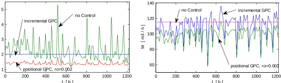
Fig. 7 shows the regulatory performance during simulat ion test when the disturbances presented in Fig. 5 a re applied.

Three cases are presented: (i) control using positional GPC (dotted line ), (ii) control using incre mental GPC (continuous line)

and (iii) no control (dashed line). The DO setpoint is fixed at 2 mg/l and is kept constant during the simu lation. The

disadvantage of using the positional GPC is the steady state error and the advantage is a low power consumption. Therefore,

choosing the control-weighting coefficient value will be based on compromise between performance and power consumption.

In the case of Fig. 7, the average amount of air necessary for aeration is 2647 cubic meters daily if incre mental GPC control is

used. Positional GPC with a value ρ=0.002 leads to an average amount of air necessary for aeration of 2348 cubic meters daily.

Considering the percentage, this means 88% of the average a mount of air necessary for aeration using incremental GPC, i.e. a

12% reduction in a ir flo w. The blo wers operate under a predictable set of laws concerning speed, power and pressure. In

accordance with affinity la ws, flow is proportional to motor speed; and power is proportional to the cube of motor speed. This

means that already min ima l reductions in blower air flow can provide savings in en ergy consumption. Reducing the blower air

flow by 12% decreases the power requirement by 32%.

Fig. 7 Regulatory performances for load disturbances presented in Fig . 5, process output (DO) and control output (W). Incremental GPC - continuous line, positional GPC with ρ=0.002 - dotted line, no control - dashed line.

10 15 20 25 30

100 110 120

t [ h ]

W

[

m

3

/

h

]

no Control incremental GPC

positional GPC, ro=0.002

10 15 20 25 30

0.7 0.8 0.9 1 1.1 1.2 1.3 1.4

t [ h ]

D

O

[

m

g

/

l

] positional GPC, ro=0.001

no control incremental GPC

0 200 400 600 800 1000 1200

1 2 3 4 5

D

O

[

m

g

/

l

]

t [ h ] incremental GPC

no Control

positional GPC, ro=0.002

0 200 400 600 800 1000 1200

60 80 100 120 140

W

[

m

3

/

h

]

t [ h ]

no Control incremental GPC

5.

Conclusions

The wastewater treatment plants are considered comple x processes due to the strong nonlinearit ies, large variable time

constants and continuous perturbations present in the influent. This study evaluates the performance of a positional GPC

control algorith m for the dissolved oxygen concentration in the activated sludge process of a WWTP. Both the setpoint

tracking and the regulatory performances have been tested and compared with those obtained using the incremental GPC. The

design parameters for both controllers are the same and the simulations provide information on the compromise between

control performances (steady state error and response time ) and savings in energy consumption. The aerat ion flo w and, by

default, the b lower’s speed is allowed to be lowered when the operatin g conditions of the WWTP permit. The power consumed

by blowers is proportional to the cube of air flo w. This means that already min ima l reductions in blo wer a ir flow can provide

savings in energy consumption.

Since the presented control system is responsible for forc ing the plant to follow the setpoint prescribed by the optimizing

part of a mult ilayer hiera rchica l control structure, it re ma ins to be analyzed in what degree the overall performances of the

hierarchical control system will be affected by the steady state error of this control loop.

Acknowledgement

The support of the Ro manian National Authority for Scientific Research, UEFISCDI, under Grant CASEAU - 274/ 2014

and PN-III-P2-2.1-CI-2017-0202 is gratefully acknowledged.

References

[1] U. Jeppsson, “Modelling aspects of wastewater treatment processes,” Ph.D. thesis, Dept. of Industrial Electrical Eng. and Automation, Lund University, Sweden, 1996.

[2] D. Brjdanovic, S. C. F. Meijer, C. M. Lopez-Va zquez, C.M. Hooijmans, M. C. M. van Loosdrecht, “Applications of

a

s

m

[3] R. Katebi, M. A. Johnson, and J. W ilkie, Control and instrumentation for wastewater treat ment plants, Springer, London, 2012.

[4] M.A. Brdys, M. Grochowski, T. Gminski, K. Konarcza k, and M. Dre wa, “ Hierarch ical predict ive control o f integrated wastewater treatment systems,” Control Engineering Practice, vol. 16, no. 6, pp. 751-767, June 2008.

[5] N. S. Iordache, C. Petrescu, G. Necula, and Busuioc, “Municipal wastewater treat ment improve ment using computer simu lating, advances in waste management,” Proc. the 4th WSEAS International Conf. Waste Management, Water Pollution, Air Pollution, Indoor Climate (WWAI’10), May 2010, pp. 95-100.

[6] I. Naşcu,G. Vlad, S. Folea , and T. Buzdugan, “Deve lopment and application of a PID auto-tuning method to a wastewater treatment process,” 2008 IEEE International Conf. Automation, Quality and Testing, Robotics, IEEE Press, August 2008, pp. 229-234.

[7] J. Kocijan, N. Hvala, and S. Strmčn ik, “Multi-model control of wastewater treat ment reactor,” System and control: theory and applications , pp. 49-54, 2000.

[8] G. Vlad, R. Crişa, B. Mureşan, I. Naşcu, and C. Dǎrab, “ Develop ment and application o f a predict ive adaptive controlle r to a wastewater treatment process,” 2010 IEEE International Conf. Automation, IEEE Press, July 2010, pp. 219-224. [9] S. M irghasemi, C. J. B. Macnab, A. Chu, “ Dissolved oxygen control of activated sludge biorectors using neural-adaptive

control,” Proc. IEEE Symp. Computational Intelligence in Control and Automation, Dec. 2014. pp. 1-6.

[10] B. Ho lenda, E. Do mo kos, A. Redey, and J. Faza kas, “Dissolved oxygen control of the activated sludge wastewater treatment process using model p redictive control,” Co mputers and Chemica l Engineering, vol. 32, no. 6, pp. 1270-1278, June2008.

[12] C. Belch ior, R. A raújo, and J. Landeck, “ Dissolved oxygen control of the activated sludge wastewater treat ment process using stable adaptive fuzzy control,” Computers and Chemical Engineering, vol. 37, pp. 152-162, February 2012. [13] G. Harja, I. Nascu, C. Muresan, and I. Nascu, “Improve ments in dissolved oxygen control of an activated sludge

wastewater treatment process,”Circuits Systems and Signal Processing, vol. 35, no. 6, pp. 2259-2281, June 2016. [14] D. W. Clarke, C. Mohtadi, and P. Tuffs, “ Generalized predictive control part 1. the basic algorith m,” Automatica, vo l. 23,

no. 2, pp. 137-148, March 1987.

[15] W. Gu jer, M. Henze, T. M ino, and M . Van Loosdrecht, Activated sludge models ASM1, ASM2, ASM 2d and ASM 3, IWA Publishing, 2000.

[16] S. Cristescu, I. Naşcu, and I. Naşcu, “Sensitivity analysis of an activated sludge model for a qastewater treatment plant,” Proc. International Conf. System Theory, Control and Computing, pp. 595-600, October 2015.

[17] I. Muntean, R. Both, R. Crisan, and I. Nascu, “ RGA analysis and decentralized control for a wastewater treatment plant,” Proc. the IEEE International Conf. Industrial Technology, March 2015, pp. 453-458.

[18] G. Ha rja , C. Mureşan, G. Vlad and I. Naşcu, “ Fract ional order PI control strategy on an activated slud ge wastewater treatment process,” 17th International Conf. System Theory, Control and Co mputing (ICSTCC), IEEE Press, October 2015.

[19] G. Harja, G. Vlad, and I. Naşcu. “Dissolved oxygen control strategy for an activated sludge wastewater treatment process ,” Recent Advances in Electrical Engineering Series. Proc. the 19th International Conf. Systems (CSCC'15), Ju ly 2015 pp.