Learning to Select Features using their Properties

Learning to Select Features using their Properties

Eyal Krupka [email protected]

Amir Navot [email protected]

Naftali Tishby [email protected]

School of Computer Science and Engineering Interdisciplinary Center for Neural Computation The Hebrew University Jerusalem, 91904, Israel

Editor: Isabelle Guyon

Abstract

Feature selection is the task of choosing a small subset of features that is sufficient to predict the target labels well. Here, instead of trying to directly determine which features are better, we attempt to learn the properties of good features. For this purpose we assume that each feature is represented by a set of properties, referred to as meta-features. This approach enables prediction of the quality of features without measuring their value on the training instances. We use this ability to devise new selection algorithms that can efficiently search for new good features in the presence of a huge number of features, and to dramatically reduce the number of feature measurements needed. We demonstrate our algorithms on a handwritten digit recognition problem and a visual object cate-gory recognition problem. In addition, we show how this novel viewpoint enables derivation of better generalization bounds for the joint learning problem of selection and classification, and how it contributes to a better understanding of the problem. Specifically, in the context of object recog-nition, previous works showed that it is possible to find one set of features which fits most object categories (aka a universal dictionary). Here we use our framework to analyze one such universal dictionary and find that the quality of features in this dictionary can be predicted accurately by its meta-features.

Keywords: feature selection, unobserved features, meta-features

1. Introduction

In many supervised learning tasks the input is represented by a very large number of features, many of which are not needed for predicting the labels. Feature selection is the task of choosing a small subset of features that is sufficient to predict the target labels well. The main motivations for feature selection are computational complexity, reducing the cost of measuring features, improved classification accuracy and problem understanding. Feature selection is also a crucial component in the context of feature extraction. In feature extraction the original input features (for example, pixels) are used to generate new, more complicated features (for example logical AND of sets of 3 binary pixels). Feature extraction is a very useful tool for producing sophisticated classification rules using simple classifiers. One main problem here is that the potential number of additional features one can extract is huge, and the learner needs to decide which of them to include in the model.

function can be based on the performance of a specific predictor (wrapper model) or on some gen-eral (typically cheaper to compute) relevance measure of the features to the prediction (filter model) (Kohavi and John, 1997). In any case, an exhaustive search over all feature sets is generally in-tractable due to the exponentially large number of possible sets. Therefore, search methods apply a variety of heuristics, such as hill climbing and genetic algorithms. Other methods simply rank individual features, assigning a score to each feature independently. These methods ignore redun-dancy and inevitably fail in situations where only a combined set of features is predictive of the target function. However, they are usually very fast, and are very useful in most real-world prob-lems, at least for an initial stage of filtering out useless features. One very common such method is Infogain (Quinlan, 1990), which ranks features according to the mutual information1_{between each} feature and the labels. Another selection method which we refer to in the following is Recursive Feature Elimination (RFE, Guyon et al., 2002). SVM-RFE is a wrapper selection methods for linear Support Vector Machine (SVM). In each round it measures the quality of the candidate features by training SVM and eliminates the features with the lowest weights. See Guyon and Elisseeff (2003) for a comprehensive overview of feature selection.

In this paper we present a novel approach to the task of feature selection. Classical methods of feature selection tell us which features are better. However, they do not tell us what characterizes these features or how to judge new features which were not measured in the training data. We claim that in many cases it is natural to represent each feature by a set of properties, which we call meta-features. As a simple example, in image-related tasks where the features are gray-levels of pixels, the(x,y)position of each pixel can be the meta-features. The value of the meta-features is fixed per feature; in other words it is not dependent on the instances. Therefore, we refer to the meta-features as prior knowledge. We use the training set to learn the relation between the meta-feature values and feature usefulness. This in turn enables us to predict the quality of unseen features. This ability is an asset particularly when there are a large number of potential features and it is expensive to measure the value of each feature. For this scenario we suggest a new algorithm called Meta-Feature based Predictive Meta-Feature Selection (MF-PFS) which is an alternative to RFE. The MF-PFS algorithm uses predicted quality to select new good features, while eliminating many low-quality features without measuring them. We apply this algorithm to a visual object recognition task and show that it outperforms standard RFE. In the context of object recognition there is an advantage in finding one set of features (referred to as a universal dictionary) that is sufficient for recognition of most kinds of objects. Serre et al. (2005) found that such a dictionary can be built by random selection of patches from natural images. Here we show what characterizes good universal features and demonstrate that their quality can be predicted accurately by their meta-features.

The ability to predict feature quality is also a very valuable tool for feature extraction, where the learner has to decide which potential complex features have a good chance of being the most useful. For this task we derive a selection algorithm (called Mufasa) that uses meta-features to explore a huge number of candidate features efficiently. We demonstrate the Mufasa algorithm on a handwritten digit recognition problem. We derive generalization bounds for the joint problem of feature selection (or extraction) and classification, when the selection uses meta-features. We show that these bounds are better than those obtained by direct selection.

The paper is organized as follows: we provide a formal definition of the framework and define some notations in Section 2. In Sections 3 and 4 we show how to use this framework to predict the

quality of individual unseen features and how this ability can be combined with RFE. In Section 5 we apply MF-PFS to an object recognition task. In Section 6 we show how the use of meta-features can be extended to sets of features, and present our algorithm for guiding feature extraction. We illustrate its abilities on the problem of handwritten digit recognition. Our theoretical results are presented in Section 7. We discuss how to choose meta-features wisely in Section 8. Finally we conclude with some further research directions in Section 9. A Matlab code running the algorithms and experiments presented in this paper is available upon request from the authors.

1.1 Related Work

Incorporating prior knowledge about the representation of objects has long been known to pro-foundly influence the effectiveness of learning. This has been demonstrated by many authors using various heuristics such as specially engineered architectures or distance measures (see, for example, LeCun et al., 1998; Simard et al., 1993). In the context of support vector machines (SVM) a variety of successful methods to incorporate prior knowledge have been published over the last ten years (see, for example, Decoste and Schölkopf 2002 and a recent review by Lauer and Bloch 2006). Krupka and Tishby (2007) proposed a framework that incorporates prior knowledge on features, which is represented by meta-features, into learning. They assume that a weight is assigned to each feature, as in linear discrimination, and they use the meta-features to define a prior on the weights. This prior is based on a Gaussian process and the weights are assumed to be a smooth function of the meta-features. While in their work meta-features are used for learning a better classifier, in this work meta-features are used for feature selection.

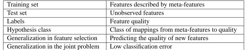
Training set Features described by meta-features

Test set Unobserved features

Labels Feature quality

Hypothesis class Class of mappings from meta-features to quality Generalization in feature selection Predicting the quality of new features

Generalization in the joint problem Low classification error

Table 1: Feature learning by meta-features as a form of standard supervised learning

2. Framework and Notation

In supervised (classification) learning it is assumed that we have a training set Sm=

xi,yi m_i=1, xi∈RN and yi=c xiwhere c is an unknown classification rule. The task is to find a mapping h fromRN to the label set with a small chance of erring on a new unseen instance, x∈RN, that was drawn according to the same probability function as the training instances. The N coordinates are called features. The standard task of feature selection is to select a subset of features that enables good prediction of the label. This is done by looking for features which are more useful than the others. We can also consider the instances as abstract entities in space

S

and think of the features as measurements on the instances. Thus each feature f can be considered as a function from

S

to

R; that is, f :

S

→R. We denote the set of all the features by{fj}N_j=1. We use the term feature to

describe both raw input variables (for example, pixels in an image) and variables constructed from the original input variables using some function (for example, product of 3 pixels in the image). We also use F to denote a set of features and Sm_F to denote the training set restricted to F; that is, each instance is described only by the features in F.

Here we assume that each feature is described by a set of k properties u(·) ={ur(·)}kr=1which we call meta-features. Formally, each ur(·)is a function from the space of possible measurements

toR. Thus each feature f is described by a vector u(f) = (u1(f), . . . ,uk(f))∈Rk. Note that the

meta-features are not dependent on the instances. As already mentioned, and will be described in detail later, this enables a few interesting applications. We also denote a general point in the image of u(·) by u. log is the base 2 logarithm while ln denotes the natural logarithm. A table that summarizes the above notations and additional notations that will be introduced later appears in Appendix B.

3. Predicting the Quality of Features

In this section we show how meta-features can be used to predict the quality of unseen features. The ability to predict the quality of features without measuring them is advantageous for many applications. In the next section we demonstrate its usage for efficient feature selection for SVM (Vapnik, 1995), when it is very expensive to measure each feature.

We assume that we observe only a subset of the N features; that is in the training set we only see the value of some of the features. We can directly measure the quality (that is, usefulness) of these features using the training set. Based on the quality of these features, our goal is to predict the quality of all features, including features that were not part of the training set. Thus we can think of the training set not only as a “training set of instances”, but also as a “training set of features”.

Algorithm 1 ˆQ=quality_map(Sm,featquality,regalg)

1. measure the feature quality vector: YMF =featquality(Sm)

2. calculate the N×k meta-features matrix XMF

3. use the regression alg. to learn a mapping from meta-feature value to quality: Qˆ =

regalg(XMF,YMF)

The quality can be based on any kind of standard evaluation function that uses the labeled training set to evaluate features (for example, Infogain or the square weights assigned by linear SVM). YMF

denotes the vector of measured qualities; that is YMF(j) is the measured quality of the j’s feature

in the training set. Now we have a new supervised learning problem, with the original features as instances, the meta-features as features and YMF as the (continuous) target label. The analogy to

the standard supervised problem is summarized in Table 1. Thus we can use any standard regression learning algorithm to find the required mapping from meta-features to quality. The above procedure is summarized in Algorithm 1. Note that this procedure uses a standard regression learning proce-dure. That is, the generalization ability to new features can be derived using standard generalization bounds for regression learning. In the next section we give a specific choice for featquality and regalg (see step 2(b) of algorithm 2).

4. Efficient Feature Selection for SVM

Support Vector Machine (SVM) (Vapnik, 1995), is one of the most prominent learning algorithms of the last decade. Many feature selection algorithms for SVM have been suggested (see, for example, Weston et al. 2000). One of the popular methods for linear SVM is Recursive Feature Elimination (Guyon et al., 2002). In SVM-RFE you start by training SVM using all the features, then eliminate the ones with the smallest square weights in the result linear classifier and repeat the same procedure with the remaining features until the set of selected features is small enough. The reason that features are eliminated iteratively and not in one step is that the weights given by SVM to a feature depend on the set of features that was used for training. Thus eliminating only a small number of the worst features in each stage minimizes the unwanted effect of this phenomenon.

Algorithm 2 ˆQ=MF-PFS(Sm,n,t,featquality,regalg)

(The algorithm selects n features out of the full set of N)

1. Initialize the set of selected features F =

fj N_j=1(all the features).

2. while|F|>n,

(a) Select a set F0of randomαn features out of F, measure them and produce a training set of features Sm_F

0.

(b) Use Algorithm 1 to produce a map ˆQ from meta-features values to quality:

ˆ

Q=quality_map(Sm_F0,featquality,regalg)

where featquality trains linear SVM and uses the resulting square weights as a measure of quality (YMF in Algorithm 1). regalg is based on k-Nearest-Neighbor Regression

(Navot et al., 2006).

(c) Use ˆQ to estimate the quality of all the features in F.

(d) Eliminate from F min(t|F|,|F| −n)features with the lowest estimated quality.

The number of measured features can be further reduced by the following method. The relative number of features we measure in each round (αin step 2(a) of the algorithm) does not have to be fixed; for example, we can start with a small value, since a gross estimation of the quality is enough to eliminate the very worst features, and then increase it in the last stages, where we fine-tune the selected feature set. This way we can save on extra feature measurements without compromising on the performance. Typical values forαmight be around 0.5 in the first iteration and slightly above 1 in the last iteration. For the same reason, in step 2(d), it makes sense to decrease the number of features we drop along the iterations. Hence, we adopted the approach that is commonly used in SVM-RFE that drops a constant fraction, t∈(0,1)of the remaining features, where a typical value of t is 0.5. An example of specific choice of parameter values is given in the next section.

5. Experiments with Object Recognition

(Gabor, 1946) of 4 different orientations and 16 different scales, followed by a local maximum of the absolute value over the location, two adjacent scales and decimation (sub-sampling). Thus, each image is replaced by 8 quadruplets of lower resolution images. Each quadruplet corresponds to one scale, and includes all 4 orientations. The following description is over this complex representation. Each feature is defined by a specific patch prototype. The prototype is one such quadruplet of a given size (4x4, 8x8, 12x12 or 16x16). The value of the feature on a new image is calculated as follows:

1. The image is converted to the above complex representation.

2. The Euclidean distance of the prototype from every possible patch (that is, at all locations and the 8 scales) of the same size in the image representation is calculated. The minimal distance (over all possible locations and scales) is denoted by d.

3. The value of the feature is e−βd2 , whereβis a parameter.

Step 2 is very computationally costly, and takes by far more resources than any other step in the process. This means that calculating the feature value on all images takes a very long time. Since each feature is defined by a prototype, the feature selection is done by selecting a set of prototypes. In Serre’s paper the features are selected randomly by choosing random patches from a data set of natural images (or the training set itself). Namely, to select a prototype you chose an image ran-domly, convert it to the above representation, then randomly select a patch from it. In Serre’s paper, after this random selection, the feature set is fixed, that is no other selection algorithm is used. One method to improve the selected set of features is to use SVM-RFE to select the best features from a larger set of randomly selected candidate features. However, since SVM-RFE requires calculating all the feature values, this option is very expensive to compute. Therefore we suggest choosing the features using meta-features by MF-PFS. The meta-features we use are:

1. The size of the patch (4, 8, 12 or 16).

2. The DC of the patch (average over the patch values).

3. The standard deviation of the patch.

4. The peak value of the patch.

5. Quantiles 0.3 and 0.7 of the values of the patch.

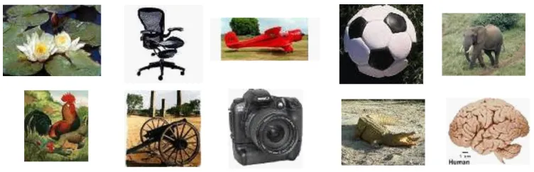
Figure 1: Excerpts from the Caltech-101 data-set

5.1 Predicting the Quality of New Features

Since the entire discussion here relies on the assumption that we can predict the quality of a feature from its meta-feature values, we first need to test whether this assumption holds. We need to prove that we can indeed predict the quality of a patch using the above meta-features; that is, from its size, DC, std, peak value and quantile values. We measure feature quality by SVM square weights of multi-class SVM (Shalev-Shwartz and Singer, 2006). Based on this quality definition, Figure 2 presents an example of prototypes of “good” and “bad” features of different sizes. In Figure 3 we explore the quality of features as a function of two meta-features: the patch size and the standard deviation (std). We can see that for small patches (4x4), more details are better, for large patches (16x16) fewer details are better and for medium size patches (for example, 8x8) an intermediate level of complexity is optimal. In other words, the larger the patch, the smaller the optimal com-plexity. This suggests that by using the size of the patch together with certain measurements of its “complexity” (for example, std) we should be able to predict its quality. In the following experiment we show that such a prediction is indeed possible.

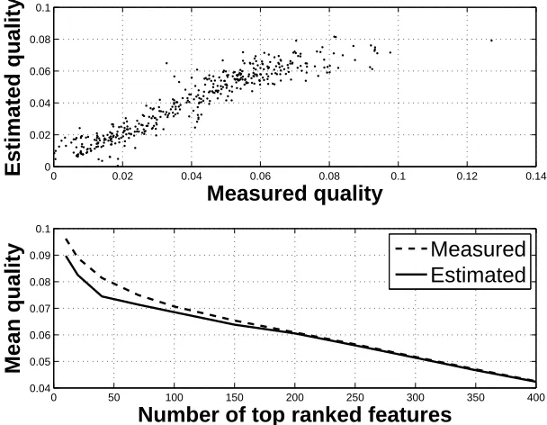
We use Algorithm 1 with the sum square of SVM weights as the direct measure for patch quality and a weighted version of k-Nearest-Neighbor Regression (Navot et al., 2006) as a regressor. To solve the SVM, we use the Shalev-Shwartz and Singer (2006) online algorithm. This algorithm has the advantage of a built-in ability to deal with multi-class problems. We use 500 features as training features. Then we use the map returned by Algorithm 1 to predict the quality of another 500 features. The results presented in Figure 4 show that the prediction is very accurate. The correlation coefficient between measured and predicted quality (on the test set of 500 features) is 0.94. We also assessed the contribution of each meta-feature, by omitting one meta-feature each time and measuring the drop in the correlation coefficient. The meta-features which contributed most to the prediction are size, mean (DC) and std.

(a) (b) (c) (d) (e)

Good 4x4 Patches

(a) (b) (c) (d) (e)

Bad 4x4 Patches

(a) (b) (c) (d) (e)

Good 16x16 Patches

(a) (b) (c) (d) (e)

Bad 16x16 Patches

Figure 2: Examples of “good” and “bad” patch prototypes of different sizes. Each row represents one patch. The left column (a) is the image from which the patch was extracted and the other 4 columns (b,c,d,e) correspond to the 4 different orientations (– / | \, respectively). Good small patches are rich in details whereas good large patches are relatively uniform.

the most useful features. However, in their work the features are object fragments, and hence their quality is dependent on the specific training set and not on general statistical properties as we found in this work.

5.2 Applying MF-PFS to Object Recognition

0 0.05 0.1 0.15 0.2 0

0.05 0.1 0.15 0.2

Standard deviation of patch levels

Quality

Patch size is 4*4

0 0.05 0.1 0.15 0.2 0

0.05 0.1 0.15 0.2

Standard deviation of patch levels

Quality

Patch size is 8*8

0 0.05 0.1 0.15 0.2 0

0.05 0.1 0.15 0.2

Standard deviation of patch levels

Quality

Patch size is 12*12

0 0.05 0.1 0.15 0.2 0

0.05 0.1 0.15 0.2

Standard deviation of patch levels

Quality

Patch size is 16*16

Figure 3: Quality as function of the standard deviation of the meta-feature. Good small patches are “complex” whereas good large patches are “simple”.

0 0.02 0.04 0.06 0.08 0.1 0.12 0.14 0

0.02 0.04 0.06 0.08 0.1

Measured quality

Estimated quality

0 50 100 150 200 250 300 350 400 0.04

0.05 0.06 0.07 0.08 0.09 0.1

Number of top ranked features

Mean quality

Measured

Estimated

We use Algorithm 2, with multi-class SVM (Shalev-Shwartz and Singer, 2006) as a classifier and the square of weights as a measure of feature quality. The regression algorithm for quality prediction is based on a weighted version of the k-Nearest-Neighbor regression (Navot et al., 2006). Since the number of potential features is virtually infinite, we have to select the initial set of N features.2 We always start with N =10n that were selected randomly from natural images in the same manner as in Serre et al. (2005). We use 4 elimination steps (follows from t =0.5, see Algorithm 2). We start with α=0.4 (see step 2(a) of the algorithm) and increase it during the iterations up toα=1.2 in the last step (values in the 2nd and 3rd iteration are 0.8 and 1 respectively). The exact values may seem arbitrary; however the algorithm is not sensitive to small changes in these values. This can be shown as follows. First note that increasing α can only improve the accuracy. Now, note also that the accuracy is bounded by the one achieved by RFEall. Thus, since the accuracy we achieve is very close to the accuracy of RFEall (see Figure 5), there is a wide range of α selection that hardly affects the accuracy. For example, our initial tests were with al pha=0.6,0.8,1,1.2 which yielded the same accuracy, while measuring almost 10% more features. General guidelines for selectingαare discussed in Section 4. For the above selected value ofα,the algorithm measures only about 2.1n features out of the 10n candidates.

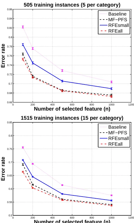
We compared MF-PFS to three different feature selection algorithms. The first was a standard RFE which starts with all the N=10n features and selects n features using 6 elimination steps (referred to as RFEall). The second method was also a standard RFE, but this time it started with 2.1n features that were selected randomly from the N=10n features (referred to as RFEsmall). The rationale for this is to compare the performance of our algorithm to standard RFE that measures the same number of features. Since standard RFE does not predict the quality of unseen features, it has to select the initial set randomly. As a baseline we also compared it to random selection of the n features as done in Serre et al. (2005) (referred to as Baseline). Note that RFEall considers all the features MF-PFS does, but makes many more measurements (with costs that become infeasible in many cases).3 On the other hand RFEsmall uses the same number of measurements as MF-PFS, but it considers about one-fifth of the potential features. Finally, in order to estimate the statistical significance of the results we repeated the whole experiment 20 times, with different splits into train instances and test instances.

Results. The results are presented in Figure 5. MF-PFS is nearly as accurate as RFEall, but uses many fewer feature measurements. When RFE measures the same number of features (RFEsmall), it needs to select twice the number of selected features (n) to achieve the same classification accuracy as MF-PFS. Recall that in this setting, as Serre et al. (2005) mentioned, measuring each feature is very expensive; thus these results represent a significant improvement.

6. Guided Feature Extraction

In the previous section we demonstrated the usefulness of meta-features in a scenario where the measurement of each feature is very costly. Here we show how the low dimensional representation of features by a relatively small number of meta-features enables efficient selection even when the number of potential features is very large or even infinite and the evaluation function is expensive (for example, the wrapper model). This is highly relevant to the feature extraction scenario. Note

2. In Section 6 we show that meta-features can be used to explore a space of an infinite number of potential features. 3. It took days on dozens of computers to measure the N=10,000 features on Caltech-101 required for RFEall. This is

0 200 400 600 800 1000 1200 0.66

0.68 0.7 0.72 0.74 0.76 0.78 0.8 0.82 0.84 0.86

Number of selected feature (n)

Error rate

505 training instances (5 per category)

Baseline MF−PFS RFEsmall RFEall

0 200 400 600 800 1000 1200

0.5 0.55 0.6 0.65 0.7 0.75 0.8 0.85

Number of selected feature (n)

Error rate

1515 training instances (15 per category)

Baseline MF−PFS RFEsmall RFEall

Figure 5: Applying SVM with different feature selection methods for object recognition. When the number of selected features (n) is not too small, our meta-feature based selection (MF-PFS) achieves the same accuracy as RFEall which measures 5 times more features at training time. MF-PFS significantly outperforms RFEsmall which measures the same number of features at training time. To get the same classification accuracy RFEsmall needs about twice the number of features that MF-PFS needs. The results of the baseline algorithm that uses random selection are also presented (Baseline). Error bars show 1-std of the mean performance over the 20 runs.

Algorithm 3 Fbest =Mufasa(n,J)

1. Initialization: qbest=maxreal, u0is the initial guess of u (In our experiments we use uniform random).

2. For j=1. . .J

(a) Select (or generate) a new set Fj of n random features according to p(v|uj−1). See Sections 6.1 and 6.2 for details.

(b) qj=quality(Fj). (Any measure of quality, In our experiment we use cross-validation

classification accuracy of SVM)

(c) If qj≥qbest

Fbest=Fj, ubest=uj−1, qbest=qj

(d) Randomly select new uj which is near ubest. For example, in our experiments we add

Gaussian random noise to each coordinate of ubest, followed by round to the nearest

valid value.

3. return Fbest

6.1 Meta-features Based Search

Assume that we want to select (or extract) a set of n features out of large number of N potential features. We define a stochastic mapping from values of meta-features to selection (or extraction) of features. More formally, let V be a random variable that indicates which feature is selected. We assume that each point u in the meta-feature space induces density p(v|u) over the features. Our goal is to find a point u in the meta-feature space such that drawing n features (independently) according to p(v|u)has a high probability of giving us a good set of n features. For this purpose we suggest the Mufasa (for Meta-Features Aided Search Algorithm) (Algorithm 3) which implements a stochastic local search in the meta-feature space.

Note that Mufasa does not use explicit prediction of the quality of unseen features as we did in MF-PFS, but it is clear that it cannot work unless the meta-features are informative on the quality. Namely, Mufasa can only work if the likelihood of drawing a good set of features from p(v|u)is some continuous function of u; that is, a small change in u results in a small change in the chance of drawing a good set of features. If, in addition, the meta-feature space is “simple”4 we expect it to find a good point in a small number of steps J. In practice, we can stop when no notable improvement is achieved in a few iterations in a row. The theoretical analysis we present later suggests that overfitting is not a main consideration in the choice of J, since the generalization bound depends on J only logarithmically.

Like any local search over a non-convex target function, convergence to a global optimum is not guaranteed, and the result may depend on the starting point u0. Note that the random noise added to u (step 2d in Algorithm 3) may help avoid local maxima. However, other standard techniques to avoid local maxima can also be used (for example, simulated annealing). In practice we found, at least in our experiments, that the results are not sensitive to the choice of u0, though it may affect

the number of iterations, J, required to achieve good results. The choice of p(v|u)is application-dependent. In the next section we show how it is done for a specific example of feature generation. For feature selection it is possible to cluster the features based on the similarity of meta-features, and then randomly select features per cluster. Another issue is how to choose the next meta-features point (step 2(d)). Standard techniques for optimizing the step size, such as gradually reducing it, can be used. However, in our experiment we simply added an independent Gaussian noise to each meta-feature.

In Section 6.2 we demonstrate the ability of Mufasa to efficiently select good features in the presence of a huge number of candidate (extracted) features on a handwritten digit recognition problem. In Section 7.1 we present a theoretical analysis of Mufasa.

6.2 Illustration on a Digit Recognition Task

In this section we use a handwritten digit recognition problem to demonstrate how Mufasa works for feature extraction. We used the MNIST (LeCun et al., 1998) data set which contains images of 28×28 pixels of centered digits(0. . .9). We converted the pixels from gray-scale to binary by thresholding. We use extracted features of the following form: logical AND of 1 to 8 pixels (or their negation), which are referred to as inputs. This creates intermediate AND-based features which are determined by their input locations. The features we use are calculated by logical OR over a set of such AND-features that are shifted in position in a shiftInfLen*shiftInvLen square. For example, assume that an AND-based feature has two inputs in positions(x1,y1)and(x2,y2), shiftInvLen=2 and both inputs are taken without negation. Thus the feature value is calculated by OR over 2*2 AND-based features as follows:

(Im(x1,y1)∧Im(x2,y2))∨(Im(x1,y1+1)∧Im(x2,y2+1))∨

(Im(x1+1,y1)∧Im(x2+1,y2))∨(Im(x1+1,y1+1)∧Im(x2+1,y2+1))

where Im(x,y)denotes the value of the image in location(x,y). This way we obtain features which are not sensitive to the exact position of curves in the image.

Thus a feature is defined by specifying the set of inputs, which inputs are negated, and the value of shiftInvLen. Similar features have already been used by Kussul et al. (2001) on the MNIST data set, but with a fixed number of inputs and without shift invariance. The idea of using shift invariance for digit recognition is also not new, and was used, for example, by Simard et al. (1996). It is clear that there are a huge number of such features; thus we have no practical way to measure or use all of them. Therefore we need some guidance for the extraction process, and this is the point where the meta-features framework comes in. We use the following four meta-features:

1. numInputs: the number of inputs (1-8).

2. percentPos: percent of logic positive pixels (0-100, rounded). 3. shiftInvLen: maximum allowed shift value (1-8).

4. scatter: average distance of the inputs from their center of gravity (COG) (1-3.5).

0

0.5

1

1.5

2

2.5

x 10

4

10

−1

Total budget

Test Error

Mufasa Rand Search Norm. Infogain Polynomial SVM

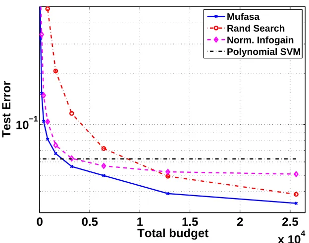
Figure 6: Guided feature extraction for digit recognition. The generalization error rate as a function of the available budget for features, using different selection methods. The number of training instances is 2000 (randomly selected from the MNIST training set). Error bars show a one standard deviation confidence interval. SVM is not limited by the budget, and always implicitly uses all the products of features. We only present the results of SVM with a polynomial kernel of degree 2, the value that gave the best results in this case.

computationally expensive. Thus a selection algorithm is restricted by a budget which the total cost of the selected set of features cannot be exceeded, rather than by an allowed number of selected features. We defined the cost of measuring (calculating) a feature as 0.5 1+a2, where a is the shiftInvLen of the feature; this way the cost is proportional to the number of locations where we measure the feature.5

We used 2000 images as a training set, and the number of steps, J, is 50. We chose specific fea-tures, given a value of meta-feafea-tures, by re-drawing features randomly from a uniform distribution over the features that satisfied the given value of the meta-features until the full allowed budget was used up. We used 2-fold cross validation of the linear multi-class SVM (Shalev-Shwartz and Singer, 2006; Crammer, 2003) to check the quality of the set of selected features in each step. Finally, for each value of allowed budget we checked the results obtained by the linear SVM on the MNIST standard test set using the selected features.

We compared the results with those obtained using the features selected by Infogain as follows. We first drew features randomly using a budget which was 50 times larger, then we sorted them by Infogain (Quinlan, 1990) normalized by the cost6 (that is, the value of Infogain divided by 5. The number of inputs does not affect the cost in our implementation since the feature value is calculated by 64-bit

logic operations.

2 3 4 1

2 3 4 5

Inputs #

(a)

2 3 4

1 2 3 4 5 6

Shift inv

(b)

2 3 4

0 50 100

% Positive

(c)

Y−axis: Optimal value

2 3 4

1 2 3 4

Scatter

(d) X−axis: Log₁₀(budget)

Figure 7: Optimal value of the different meta-features as a function of the budget. The results are averaged over 20 runs, and the error bars indicate the range where values fall in 80% of the runs. The size of the optimal shift invariance and the optimal number inputs increases with the budget.

computational cost of calculating the feature as defined above). We then selected the prefix that used the allowed budget. This method is referred to as Norm Infogain. As a sanity check, we also compared the results to those obtained by doing 50 steps of choosing features of the allowed budget randomly; that is, over all possible values of the meta-features. Then we used the set with the lowest 2-fold cross-validation error (referred to as Rand Search). We also compared our results to SVM with a polynomial kernel of degree 1-8, that uses the original pixels as input features. This comparison is relevant since SVM with a polynomial kernel of degree k implicitly uses ALL the products of up to k pixels, and the product is equal to AND for binary pixels. To evaluate the statistical significance, we repeated each experiment 20 times, with a different random selection of training sets out of the standard MNIST training set. For the test set, we use the entire 10,000 test instances of the MNIST data set. The results are presented in Figure 6. It is clear that Mufasa outperforms the budget-dependent alternatives, and outperforms SVM for budgets larger than 3000 (about 600 features). It is worth mentioning that our goal here is not to compete with the state-of-art results on MNIST, but to illustrate our concept and to compare the results for the same kind of classifier with and without using our meta-features guided search. Note that our concept can be combined with most kinds of classification, feature selection, and feature extraction algorithms to improve them, as discussed in Section 9.

the available budget. Figure 7 presents the average chosen value of each meta-feature as a function of the budget. As shown in Figure 7b, when the budget is very limited, it is better to take more cheap features rather than fewer more expensive shift invariant features. On the other hand, when we increase the budget, adding these expensive complex features is worth it. We can also see that when the budget grows, the optimal number of inputs increases. This occurs because for a small budget, we prefer features that are less specific, and have relatively high entropy, at the expense of “in class variance”. For a large budget, we can permit ourselves to use sparse features (low probability of being 1), but with a gain in specificity. For the scatter meta-features, there is apparently no correlation between the budget and the optimal value. The vertical lines (error bars) represent the range of selected values in the different runs. It gives us a sense of the importance of each meta-feature. A smaller error bar indicates higher sensitivity of the classifier performance to the value of the meta-feature. For example, we can see that performance is sensitive to shiftInvLen and relatively indifferent to percentPos.

7. Theoretical Analysis

In this section we derive generalization bounds for the combined process of selection and classifica-tion when the selecclassifica-tion process is based on meta-features. We show that in some cases, these bounds are far better than the bounds that assume each feature can be selected directly. This is because we can significantly narrow the number of possible selections, and still find a good set of features. In Section 7.1 we analyzed the case where the selection is made using Mufasa (Algorithm 3). In Sec-tion 7.2 we present a more general analysis, which is independent of the selecSec-tion algorithm, and instead assumes that we have a given class of mappings from meta-features to a selection decision.

7.1 Generalization Bounds for Mufasa Algorithm

The bounds presented in this section assume that the selection is made using Mufasa (Algorithm 3), but they could be adapted to other meta-feature based selection algorithms. Before presenting the bounds, we need some additional notations. We assume that the classifier that is going to use the selected features is chosen from a hypothesis class

H

cof real valued functions and the classification

is made by taking the sign.

We also assume that we have a hypothesis class

H

f s, where each hypothesis is one possible way

to select the n out of N features. Using the training set, our feature selection is limited to selecting one of the hypotheses that is included in

H

f s. As we show later, if

H

f scontains all the possible ways

of choosing n out of N features, then we get an unattractive generalization bound for large values of n and N. Thus we use meta-features to further restrict the cardinality (or complexity) of

H

f s. We

have a combined learning scheme of choosing both hc∈

H

c and hf s∈

H

f s. We can view this as

choosing a single classifier from

H

f s×

H

c. In the following paragraphs we analyze the equivalent

size of hypothesis space

H

f sof Mufasa as a function of the number of steps in the algorithm.

For the theoretical analysis, we need to bound the number of feature selection hypotheses Mu-fasa considers. For this purpose, we reformulate MuMu-fasa as follows. First, we replace step 2(a) with an equivalent deterministic step. To do so, we add a “pre-processing” stage that generates (randomly) J different sets of features of size n according to p(v|u) for any possible value of the point u in the meta-feature space.7 Now, in step 2(a) we simply use the relevant set, according to

the current u and current j. Namely, in step j we use the jth set of features that was created in the pre-processing stage according to p(v|uj), where uj is the value of u in this step. Note that the

resulting algorithm is identical to the original Mufasa, but this new formulation simplifies the theo-retical analysis. The key point here is that the pre-processing is done before we see the training set, and that now Mufasa can only select one of the feature sets created in the pre-processing. Therefore, the size of

H

f s, denoted by|

H

f s|, is the number of hypotheses created in pre-processing.

The following two lemmas upper bound|

H

f s|, which is a dominant quantity in the

generaliza-tion bound. The first one handles the case where the meta-features have discrete values, and there are a relatively small number of possible values for the meta-features. This number is denoted by |MF|.

Lemma 1 Any run of Mufasa can be duplicated by first generating J|MF|hypotheses and then running Mufasa using these hypotheses alone; that is, using|

H

f s| ≤J|MF|, where J is the number

of iterations made by Mufasa and|MF|is the number of different values the meta-features can be assigned.

Proof

We first generate J random feature sets for each of the |MF|possible values of meta-features. The total number of sets we get is J|MF|. We have only J iterations in the algorithm, and we generated J feature sets for each possible value of the meta-features. This guarantees that all the hypotheses required by Mufasa are available.

Note that in order to use the generalization bound of the algorithm, we cannot only consider the subset of J hypotheses that was tested by the algorithm. This is because this subset of hypotheses is affected by the training set (just as one cannot choose a single hypothesis using the training set, and then claim that the hypothesis space of the classifier includes only one hypothesis). However, from Lemma 1, the algorithm search is within no more than J|MF|feature selection hypotheses that were determined without using the training set.

The next lemma handles the case where the cardinality of all possible values of meta-features is large relative to 2J, or even infinite. In this case we can get a tighter bound that depends on J but not on|MF|.

Lemma 2 Any run of Mufasa can be duplicated by first generating 2J−1hypotheses and then run-ning Mufasa using only these hypotheses; that is, using|

H

f s| ≤2J−1, where J is the number of

iterations Mufasa performs.

The proof of this lemma is based on PAC-MDL bounds (Blum and Langford, 2003). Briefly, a codebook that maps between binary messages and hypotheses is built without using the training set. Thus, the generalization bound then depends on the length of the message needed to describe the selected hypothesis. For a fixed message length, the upper bound on the number of hypotheses is 2l where l is the length of the message in bits.

Proof

simply get the next stored random number. After this pre-processing, the feature set, which is the output of Mufasa, can be one of 2J−1previously determined sets, since it only depends on the J−1 binary decisions in step 2(c) of the algorithm (in the first iteration the decision of step 2(c) is fixed, hence we only have J−1 decisions that depend on the training set). Thus, we can generate these 2J−1hypotheses before we see the training set.

Using the above PAC-MDL technique, we can also reformulate the last part of the proof by showing that each of the feature-set hypotheses can be uniquely described by J−1 binary bits, which describes the decisions in step 2(c). A better generalization bound can be obtained if we assume that in the last steps a new hypothesis will rarely be better than the stored one, and hence the probability of replacing the hypothesis in step 2(c) is small. In this case, we can get a data-dependent bound that usually increases more slowly with the number of iterations (J), since the entropy of the message describing the hypothesis is likely to increase slowly for large J.

To state our theorem we also need the following standard definitions:

Definition 3 Let

D

be a distribution over

S

× {±1}and h :

S

→ {±1}a classification function. We denote by er_D(h)the generalization error of h w.r.t

D

:

er_D(h) =Prs,y∼D[h(s)6=y].

For a sample Sm={(sk,yk)}mk=1∈(

S

× {±1})

m_{and a constantγ>0, theγ-sensitive training error}

is:

ˆ

erγ_S(h) = 1

m|{i : h(si)6=yi} or

(si has sample-margin<γ),|

where the sample-margin measures the distance between the instance and the decision boundary induced by the classifier.

Now we are ready to present the main result of this section:

Theorem 4 Let

H

cbe a class of real valued functions. Let S be a sample of size m generated i.i.d

from a distribution

D

over

S

× {±1}. If we choose a set of features using Mufasa, with a probability of 1−δover the choices of S, for every hc∈

H

cand everyγ∈(0,1]:

er_D(hc)≤erˆγS(hc)+

s

2 m

d ln

34em d

log(578m) +ln

8 γδ

+g(J)

,

where

• g(J) =min(J ln 2,ln(J|MF|)) (where J is the number of steps Mufasa makes and|MF|is the number of different values the meta-features can be assigned, if this value is finite, and∞ otherwise).

Our main tool in proving the above theorem is the following theorem:

Theorem 5 (Bartlett, 1998)

Let

H

be a class of real valued functions. Let S be a sample of size m generated i.i.d from a distribution

D

over

S

× {±1}; then with a probability of 1−δover the choices of S, every h∈

H

and everyγ∈(0,1]:

er_D(h)≤erˆγ_S(h)+

s 2 m d ln 34em d

log(578m) +ln

8 γδ

,

where d= f at_H (γ/32)

Proof (of theorem 4) LetnF1, ...,F|Hf s|

o

be all possible subsets of the selected features. From Theorem 5 we know that

er_D(hc,Fi)≤erˆγ_S(hc,Fi)+

s 2 m d ln 34em d

log(578m) +ln

8 γδFi

,

where er_D(hc,Fi)denotes the generalization error of the selected hypothesis for the fixed set of

features Fi.

By choosingδF=δ/|

H

f s|and using the union bound, we get that the probability that there exist

Fi (1≤i≤ |

H

f s|) such that the equation below does not hold is less thanδ

er_D(hc)≤erˆγS(hc) +

s 2 m d ln 34em d

log(578m) +ln

8 γδ

+ln|

H

f s|

.

Therefore, with a probability of 1−δthe above equation holds for any algorithm that selects one of the feature sets out of nF1, ...,F|Hf s|

o

. Substituting the bounds for |

H

f s|from Lemma 1 and

Lemma 2 completes the proof.

An interesting point in this bound is that it is independent of the total number of possible fea-tures, N (which may be infinite in the case of feature generation). Nevertheless, it can select a good set of features out of O 2J

7.2 VC-dimension of Joint Feature Selection and Classification

In the previous section we presented an analysis which assumes that the selection of features is made using Mufasa. In this section we turn to a more general analysis, which is independent of the specific selection algorithm, and rather assumes that we have a given class

H

sof mappings from

meta-features to a selection decision. Formally,

H

sis a class of mappings from meta-feature value to

{0,1}; that is, for each hs∈

H

s,hs::Rk→ {0,1}. hsdefines which features are selected as follows:

f is selected⇐⇒hs(u(f)) =1,

where, as usual, u(f)is the value of the features for feature f . Given the values of the meta-features of all the meta-features together with hswe get a single feature selection hypothesis. Therefore,

H

sand the set of possible values of meta-features indirectly defines our feature selection hypothesis

class,

H

f s. Since we are interested in selecting exactly n features (n is predefined), we use only a

subset of

H

swhere we only include functions that imply the selection of n features.8For simplicity,

in the analysis we use the VC-dim of

H

swithout this restriction, which is an upper bound of the

VC-dim of the restricted class.

Our goal is to calculate an upper bound on the VC-dimension (Vapnik, 1998) of the joint prob-lem of feature-selection and classification. To achieve this, we first derive an upper bound on

H

_{f s}

as a function of VC-dim(

H

s)and the number of features N.

Lemma 6 Let

H

sbe a class of mappings from the meta-feature space (Rk) to{0,1}, and let

H

f sbe

the induced class of feature selection schemes; the following inequality holds:

H

_{f s}

≤

eN VC-dim(

H

s)

VC-dim(Hs)

.

Proof

The above inequality follows directly from the well known fact that a class with VC-dim d cannot produce more than em_d ddifferent partitions of a sample of size m (see, for example, Kearns and Vazirani 1994 pp. 57).

The next lemma relates the VC dimension of the classification concept class (dc), the cardinality

of the selection class (

H

_{f s}

) and the VC-dim of the joint learning problem.

Lemma 7 Let

H

f s be a class of the possible selection schemes for selecting n features out of N

and let

H

c be a class of classifiers over Rn. Let dc =dc(n) be the VC-dim of

H

c. If dc ≥11

then the VC-dim of the combined problem (that is, choosing(hf s,hc)∈

H

f s×

H

c) is bounded by (dc+log|

H

f s|+1)log dc.

The proof of this lemma is given in Appendix A.

Now we are ready to state the main theorem of this section.

8. Note that one valid way to defineHsis by applying a threshold on a class of mappings from meta-feature values to

Theorem 8 Let

H

s be a class of mappings from the meta-feature space (Rk) to{0,1}, let

H

f s be

the induced class of feature selection schemes for selecting n out of N features and let

H

cbe a class

of classifiers overRn. Let dc=dc(n)be the VC-dim of the

H

c. If dc≥11, then the VC-dim of the

joint class

H

f s×

H

c is upper bounded as follows

VC-dim(

H

f s×

H

c)≤

dc+dslog

eN ds

+1

log dc,

where dsis the VC-dim of

H

s.

The above theorem follows directly by substituting Lemma 6 in Lemma 7.

To illustrate the gain of the above theorem we calculate the bound for a few specific choices of

H

sand

H

c:

1. First, note that if we do not use meta-features, but consider all the possible ways to select n out of N features the above bound is replaced by

dc+log

N n

+1

log dc, (1)

which is very large for reasonable values of N and n.

2. Assuming that both

H

sand

H

care classes of linear classifiers onRkandRnrespectively, then

ds=k+1 and dc=n+1 and we get that the VC of the combined problem of selection and

classification is upper bounded by

O( (n+k log N)log n).

If

H

cis a class of linear classifiers, but we allow any selection of n features the bound is (by

substituting in 1):

O((n+n log N)log n),

which is much larger if kn. Thus in the typical case where the number of meta-features is much smaller than the number of selected features (for example in Section 6.2) the bound for meta-feature based selection is much smaller.

3. Assuming that the meta-features are binary and

H

sis the class of all possible functions from

meta-feature to{0,1}, then ds=2kand the bound is

O dc+2klog N

log dc

,

which is still much better than the bound in equation 1 if klog n.

8. Choosing Good Meta-features

the difficult and crucial problem of finding a good representation. It gives us a systematic way to incorporate prior knowledge about the features in the feature selection and extraction process. It also enables us to use the acquired experience in order to guide the search for good features. The fact that the number of meta-features is typically significantly smaller than the number of features makes it easy to understand the results of the feature selection process. It is easier to guess which properties might be indicative of feature quality than to guess which exact features are good. Nevertheless, the whole concept can work only if we use “good” meta-features, and this requires design. In Sections 5 and 6.2 we demonstrated how to choose meta features for specific problems. In this section we give general guidelines on good choices of features and mappings from meta-feature values to selection of meta-features.

First, note that if there is no correlation between meta-features and quality, the meta-features are useless. In addition, if any two features with the same value of meta-features are redundant (highly correlated), we gain almost nothing from using a large set of them. In general, there is a trade-off between two desired properties:

1. Features with the same value of meta-features have similar quality.

2. There is low redundancy between features with the same value of meta-features.

When the number of features we select is small, we should not be overly concerned about redundancy and rather focus on choosing meta-features that are informative on quality. On the other hand, if we want to select many features, redundancy may be dominant, and this requires our attention. Redundancy can also be tackled by using a distribution over meta-features instead of a single point.

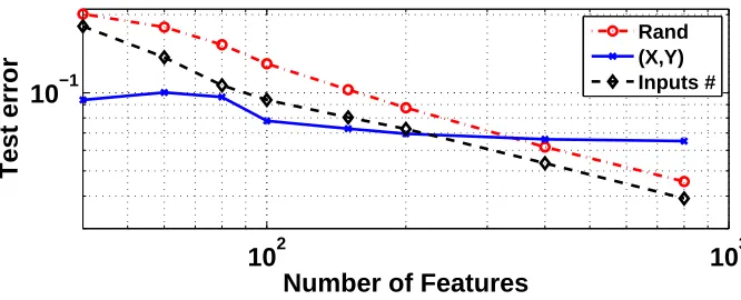
In order to demonstrate the above trade-off we carried out one more experiment using the MNIST data set. We used the same kind of features as in Section 6.2, but this time without shift-invariance and with fixed scatter. The task was to discriminate between 9 and 4 and we used 200 images as the training set and another 200 as the test set. Then we used Mufasa to select features, where the meta-features were either the (x,y)-location or the number of inputs. When the meta-feature was the(x,y)-location, the distribution of selecting the features, p(v|u), was uniform in a 4×4 window around the chosen location (step 2a in Mufasa). Then we checked the classification error on the test set of a linear SVM (which uses the selected features). We repeated this experiment for different numbers of features.9 _{The results are presented in Figure 8. When we use a small} number of features, it is better to use the(x,y)-location as a meta-feature whereas when using many features it is better to use the number of inputs as a meta-feature. This supports our contention about the redundancy-homogeneity trade-off. The(x,y)-locations of features are good indicators of their quality, but features from similar positions tend to be redundant. On the other hand, constraints on the number of inputs are less predictive of feature quality but do not cause redundancy.

9. Summary and Discussion

In this paper we presented a novel approach to feature selection. Instead of merely selecting a set of better features out of a given set, we suggest learning the properties of good features. This approach can be used for predicting the quality of features without measuring them even on a single instance.

102 103 10−1

Number of Features

Test error

Rand (X,Y) Inputs #

Figure 8: Different choices of meta-features. The generalization error as a function of the number of selected features. The two lines correspond to using different meta-features: (x,y) -location or number of inputs. The results of random selection of features are also pre-sented.

We suggest exploring for new good features by assessing features with meta-feature values similar to those of known good features. Based on this idea, we presented two new algorithms that use feature prediction. The first algorithm is MF-PFS, which estimates the quality of individual features and obviates the need to calculate them on the instances. This is useful when the computational cost of measuring each feature is very high. The second algorithm is Mufasa, which efficiently searches for a good feature set without evaluating individual features. Mufasa is very helpful in feature extraction, where the number of potential features is huge. Further, it can also help avoiding overfitting in the feature selection task.

In the context of object recognition we showed that the feature (patch) quality can be predicted by its general statistical properties which are not dependent on the objects we are trying to recognize. This result supports the existence of a universal set of features (universal-dictionary) that can be used for recognition of most objects. The existence of such a dictionary is a key issue in computer vision and brain research. We also showed that when the selection of features is based on meta-features it is possible to derive better generalization bounds on the combined problem of selection and classification.

In Section 6 we used meta-features to guide feature selection. Our search for good features is computationally efficient and has good generalization properties because we do not examine each individual feature. However, avoiding examination of individual features may also be considered as a disadvantage since we may include some useless individual features. This can be solved by using a meta-features guided search as a fast but rough filter for good features, and then applying more computationally demanding selection methods that examine each feature individually.

In Krupka and Tishby (2007) meta-features were used to build a prior on the weight assigned to each feature by a linear classifier. In that study, the assumption was that meta-features are infor-mative about the feature weights (including sign). In this work, however, meta-features should be informative about feature relevance, and the exact weight (and sign) is not important. An interesting future research direction would be to combine these concepts of using meta-features into a single framework.

tissue classification according to a gene expression array where each gene is one feature, ontology-based properties may serve as meta-features. In most cases in this domain there are many genes and very few training instances; therefore standard feature selection methods tend to over-fit and thus yield meaningless results (Ein-Dor et al., 2006). A meta-feature based selection can help as it may reduce the complexity of the class of possible selections.

In addition to the applications presented here which involve predicting the quality of unseen features, the meta-features framework can also be used to improve estimation of the quality of features that we do see in the training set. We suggest that instead of using direct quality estimation, we use some regression function on the meta-feature space (as in Algorithm 1). When we have only a few training instances, direct approximation of the feature quality is noisy; thus we expect that smoothing the direct measure by using a regression function of the meta-features may improve the approximation.

Appendix A. A Proof for Lemma 7

Lemma 7 Let

H

f s be a class of the possible selection schemes for selecting n features out of N

and let

H

c be a class of classifiers over Rn. Let dc =dc(n) be the VC-dim of

H

c. If dc ≥11

then the VC-dim of the combined problem (that is, choosing(hf s,hc)∈

H

f s×

H

c) is bounded by (dc+log|

H

f s|+1)log dc.

Proof

For a given set of selected features, the possible number of classifications of m instances is upper

bounded

em dc

dc

(see Kearns and Vazirani 1994 pp. 57). Thus, for the combined learning problem,

the total number of possible classifications of m instances is upper bounded by|

H

f s|

em dc

dc

. The

following chain of inequalities shows that if m= dc+log

H

_{f s}

+1

log dcthen

H

_{f s}

em dc dc

<2m:

|

H

f s|

e(dc+log|

H

f s|+1)log dc

dc

dc

= |

H

f s|(e log dc)dc

1+log|

H

f s|+1

dc

dc

≤ e(|

H

f s|)1+log e(e log dc)dc (2)

≤ (|

H

f s|)2+log e(e log dc)dc (3)

≤ (|

H

f s|)2+log edcdc+1 (4)

≤ ddc+1

c (|

H

f s|)log dc (5)

= ddc+1

c d

(log|Hf s|)

c (6)

= 2(dc+1+log|Hf s|)log dc_,

where we used the following equations / inequalities: (2)(1+a/d)d_≤ea _∀a,d>0

(3) here we assume|

H

f s|>e, otherwise the lemma is trivial

(6) alog b=blog a ∀a,b>1 Therefore, dc+log

H

_{f s}

+1

log dc is an upper bound on VC-dim of the combined learning

problem.

Appendix B. Notation Table

The following table summaries the notation and definitions introduced in the paper for quick refer-ence.

Notation Short description Sections

meta-feature a property that describes a feature N total number of candidate features n number of selected features k number of meta-features m number of training instances

S

(abstract) instance space 2, 7.1

f a feature: formally, f :

S

→R

c a classification rule

Sm Smis a labeled set of instances (a training set) 2, 3, 7.1 ui(f) the the value of thei’s meta-feature on feature f 2, 6 u(f) u(f) = (u1(f), . . . ,uk(f)), a vector that describes the feature f 2, 6, 7.1 u a point (vector) in the meta-feature space 2, 6

ˆ

Q a mapping from meta-features value to feature quality 3, 7.2 YMF measured quality of the features (for instance Infogain) 3

XMF XMF(i,j) =the value of the j’s meta-feature on the i’s feature 3

F,Fj a set of features 6

V a random variable indicating which features are selected 6 p(v|u) the conditional distribution of V given meta-features values (u) 6, 8

hc a classification hypothesis 7.1

H

c the classification hypothesis class 7.1

dc the VC-dimension of

H

c 7.2

hf s a feature selection hypothesis - says which n features are selected 7.1

H

f s The feature selection hypothesis class 7.1

hs A mapping form meta-feature space to{0,1} 7.2

H

s Class of mappings from meta-feature space to{0,1} 7.2

ds The VC-dimension of

H

s

J number of iteration Mufasa (Algorithm 3) does 6, 7.1 |MF| Number of possible different values of meta-features 7.1

er_D(h) generalization error of h 7.1

ˆ

References

P.L. Bartlett. The size of the weights is more important than the size of the network. IEEE Trans-actions on Information Theory, 1998.

A. Blum and J. Langford. Pac-mdl bounds. Learning Theory and Kernel Machines, 2003.

K. Crammer. Mcsvm_1.0: C code for multiclass svm, 2003. http://www.cis.upenn.edu/∼crammer.

D. Decoste and B. Schölkopf. Training invariant support vector machines. Machine Learning, 2002.

L. Ein-Dor, O. Zuk, and E. Domany. Thousands of samples are needed to generate a robust gene list for predicting outcome in cancer. Proceedings of the National Academy of Sciences, 2006.

D. Gabor. Theory of communication. J. IEE, 93:429–459, 1946.

R. Gilad-Bachrach, A. Navot, and N. Tishby. Margin based feature selection - theory and algorithms. In International Conference on Machine Learning (ICML), 2004.

R. Greiner. Using value of information to learn and classify under hard budgets. In NIPS Workshop on Value of Information in Inference, Learning and Decision-Making, 2005.

I. Guyon and A. Elisseeff. An introduction to variable and feature selection. Journal of Machine Learning Research, 2003.

I. Guyon, J. Weston, S. Barnhill, and V. Vapnik. Gene selection for cancer classification using support vector machines. Machine Learning, 46, 2002.

M. W. Kadous and C. Sammut. Classification of multivariate time series and structured data using constructive induction. Machine Learning, 2005.

M. J. Kearns and U. V. Vazirani. An Introduction to Computational Learning Theory. MIT Press, Cambridge, MA, USA, 1994.

R. Kohavi and G.H. John. Wrapper for feature subset selection. Artificial Intelligence, 97(1-2): 273–324, 1997.

E. Krupka and N. Tishby. Generalization from observed to unobserved features by clustering. Journal of Machine Learning Research, 2008.

E. Krupka and N. Tishby. Incorporating prior knowledge on features into learning. In International Conference on Artificial Intelligence and Statistics (AISTATS), 2007.

E. Kussul, T. Baidyk, L. Kasatkina, and V. Lukovich. Rosenblatt perceptrons for handwritten digit recognition. In Int’l Joint Conference on Neural Networks, pages 1516–20, 2001.

F. Lauer and G. Bloch. Incorporating prior knowledge in support vector machines for classification: a review. Submitted to Neurocomputing, 2006.