New Algorithms for Efficient High-Dimensional
Nonparametric Classification
Ting Liu [email protected]
Andrew W. Moore [email protected]
Alexander Gray [email protected]
Computer Science Department Carnegie Mellon University Pittsburgh, PA 15213, USA
Editor: Claire Cardie
Abstract
This paper is about non-approximate acceleration of high-dimensional nonparametric operations such as k nearest neighbor classifiers. We attempt to exploit the fact that even if we want exact answers to nonparametric queries, we usually do not need to explicitly find the data points close to the query, but merely need to answer questions about the properties of that set of data points. This offers a small amount of computational leeway, and we investigate how much that leeway can be exploited. This is applicable to many algorithms in nonparametric statistics, memory-based learn-ing and kernel-based learnlearn-ing. But for clarity, this paper concentrates on pure k-NN classification. We introduce new ball-tree algorithms that on real-world data sets give accelerations from 2-fold to 100-fold compared against highly optimized traditional ball-tree-based k-NN . These results in-clude data sets with up to 106dimensions and 105records, and demonstrate non-trivial speed-ups while giving exact answers.
keywords: ball-tree, k-NN classification
1. Introduction
Nonparametric models have become increasingly popular in the statistics and probabilistic AI com-munities. These models are extremely useful when the underlying distribution of the problem is unknown except that which can be inferred from samples. One simple well-known nonparametric classification method is called the k-nearest-neighbors or k-NN rule. Given a data set V ⊂RD con-taining n points, it finds the k closest points to a query pointq∈RD, typically under the Euclidean
methods (Woods et al., 1997). However, these methods all remain hampered by their computational complexity.
Several effective solutions exist for this problem when the dimension D is small, including Voronoi diagrams (Preparata and Shamos, 1985), which work well for two dimensional data. Other meth-ods are designed to work for problems with moderate dimension (i.e. tens of dimensions), such as k-D tree (Friedman et al., 1977; Preparata and Shamos, 1985), R-tree (Guttman, 1984), and ball-tree (Fukunaga and Narendra, 1975; Omohundro, 1991; Uhlmann, 1991; Ciaccia et al., 1997). Among these tree structures, balltree, or metric-tree (Omohundro, 1991), represent the practical state of the art for achieving efficiency in the largest dimension possible (Moore, 2000; Clarkson, 2002) without resorting to approximate answers. They have been used in many different ways, in a variety of tree search algorithms and with a variety of “cached sufficient statistics” decorating the internal leaves, for example in Omohundro (1987); Deng and Moore (1995); Zhang et al. (1996); Pelleg and Moore (1999); Gray and Moore (2001). However, many real-world problems are posed with very large dimensions that are beyond the capability of such search structures to achieve sub-linear efficiency, for example in computer vision, in which each pixel of an image represents a dimension. Thus, the high-dimensional case is the long-standing frontier of the nearest-neighbor problem.
With one exception, the proposals involving tree-based or other data structures have considered the generic nearest-neighbor problem, not that of nearest-neighbor classification specifically. Many proposals designed specifically for nearest-neighbor classification have been proposed, virtually all of them pursuing the idea of reducing the number of training points. In most of these approaches, such as Hart (1968), although the runtime is reduced, so is the classification accuracy. Several sim-ilar training set reduction schemes yielding only approximate classifications have been proposed (Fisher and Patrick, 1970; Gates, 1972; Chang, 1974; Ritter et al., 1975; Sethi, 1981; Palau and Snapp, 1998). Our method achieves the exact classification that would be achieved by exhaus-tive search for the nearest neighbors. A few training set reduction methods have the capability of yielding exact classifications. Djouadi and Bouktache (1997) described both approximate and exact methods, however a speedup of only about a factor of two over exhaustive search was reported for the exact case, for simulated, low-dimensional data. Lee and Chae (1998) also achieves exact clas-sifications, but only obtained a speedup over exhaustive search of about 1.7. It is in fact common among the results reported for training set reduction methods that only 40-60% of the training points can be discarded, i.e. no important speedups are possible with this approach when the Bayes risk is not insignificant. Zhang and Srihari (2004) pursued a combination of training set reduction and a tree data structure, but is an approximate method.
In this paper, we propose two new ball-tree based algorithms, which we’ll call KNS2 and KNS3. They are both designed for binary k-NN classification. We only focus on binary case, since there are many binary classification problems, such as anomaly detection (Kruegel and Vigna, 2003), drug activity detection (Komarek and Moore, 2003); and video segmentation (Qi et al., 2003). Liu et al. (2004b) applied similar ideas to many-class classification and proposed a variation of the
k-NN algorithm. KNS2 and KNS3 share the same insight that the task of k-nearest-neighbor
clas-sification of a queryqneed not require us to explicitly find those k nearest neighbors. To be more
neigh-bors ofq?” (b) “How many of the k nearest neighbors ofqare from the positive class?” and (c) “Are at least t of the k nearest neighbors from the positive class?” Many researches have focused
on the first question (a), but uses of proximity queries in statistics far more frequently require (b) and (c) types of computations. In fact, for the k-NN classification problem, when the threshold t is set, it is sufficient to just answer the much simpler question (c). The triangle inequality underlying a ball-tree has the advantage of bounding the distances between data points, and can thus help us estimate the nearest neighbors without explicitly finding them. In our paper, we test our algorithms on 17 synthetic and real-world data sets, with dimensions ranging from 2 to 1.1×10⁶and number of data points ranging from 104to 4.9×10⁵. We observe up to 100-fold speedup compared against highly optimized traditional ball-tree-based k-NN , in which the neighbors are found explicitly.
Omachi and Aso (2000) proposed a fast k-NN classifier based on a branch and bound method, and the algorithm shares some ideas of KNS2, but it did not fully explore the idea of doing k-NN classifi-cation without explicitly finding the k nearest neighbor set, and the speed-up the algorithm achieved is limited. In section 4, we address Omachi and Aso’s method in more detail.
We will first describe ball-trees and this traditional way of using them (which we call KNS1), which computes problem (a). Then we will describe a new method (KNS2) for problem (b), designed for the common setting of skewed-class data. We’ll then describe a new method (KNS3) for problem (c), which removes the skewed-class assumption, applying to arbitrary classification problems. At the end of Section 5 we will say a bit about the relative value of KNS2 versus KNS3.
2. Ball-Tree
A ball-tree (Fukunaga and Narendra, 1975; Omohundro, 1991; Uhlmann, 1991; Ciaccia et al., 1997; Moore, 2000) is a binary tree where each node represents a set of points, called Points(Node). Given a data set, the root node of a ball-tree represents the full set of points in the data set. A node can be either a leaf node or a non-leaf node. A leaf node explicitly contains a list of the points represented by the node. A non-leaf node has two children nodes: Node.child1 and Node.child2, where
Points(Node.child1)∩Points(Node.child2) =φ
Points(Node.child1)∪Points(Node.child2) =Points(Node)
Points are organized spatially. Each node has a distinguished point called a Pivot. Depending on the implementation, the Pivot may be one of the data points, or it may be the centroid of Points(Node). Each node records the maximum distance of the points it owns to its pivot. Call this the radius of the node
Node.Radius= max
x∈Points(Node)|Node.Pivot−x|
Nodes lower down the tree have smaller radius. This is achieved by insisting, at tree construction time, that
x∈Points(Node.child1) ⇒ |x−Node.child1.Pivot| ≤ |x−Node.child2.Pivot|
Provided that our distance function satisfies the triangle inequality, we can bound the distance from a query pointqto any point in any ball-tree node. If x∈Points(Node) then we know that:
|x−q| ≥ |q−Node.Pivot| −Node.Radius (1) |x−q| ≤ |q−Node.Pivot|+Node.Radius (2)
Here is an easy proof of the inequality. According to triangle inequality, we have|x−q| ≥ |q− Node.Pivot| − |x−Node.Pivot|. Given x∈Points(Node) and Node.Radius is the maximum distance
of the points it owns to its pivot,|x−Node.Pivot| ≤Node.Radius, so |x−q| ≥ |q−Node.Pivot| − Node.Radius. Similarly, we can prove Equation (2).
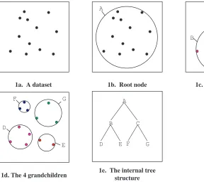
A ball-tree is constructed top-down. There are several ways to construct them, and practical al-gorithms trade off the cost of construction (it can be inefficient to be O(R2)given a data set with R points, for example) against the tightness of the radius of the balls. Moore (2000) describes a fast way for constructing a ball-tree appropriate for computational statistics. If a ball-tree is balanced, then the construction time is O(CR log R), where C is the cost of a point-point distance computation (which is O(m)if there are m dense attributes, and O(f m)if the records are sparse with only frac-tion f of attributes taking non-zero value). Figure 1 shows a 2-dimensional data set and the first few levels of a ball-tree.
1a. A dataset
A
1b. Root node
B
C
1c. The 2 children
D
G
E F
1d. The 4 grandchildren
A
B C
D E F G
1e. The internal tree structure
Figure 1: An example of ball-tree structure
3. KNS1: Conventional k Nearest Neighbor Search with Ball-Tree
Say that PS consists of the k-NN ofqin V if and only if
|V |≥k and PS are the k-NN ofqin V or
|V |<k and PS==V
(3)
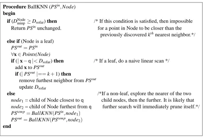
We now define a recursive procedure called BallKNN with the following inputs and output.
PSout=BallKNN(PSin,Node)
Let V be the set of points searched so far, on entry. Assume that PSinconsists of the k-NN ofqin V.
This function efficiently ensures that on exit, PSout consists of the k-NN ofqin V∪Points(Node).
We define
Dsofar=
∞
i f |PSin|<k
maxx∈PSin|x−q| i f |PSin|==k (4) Dsofaris the minimum distance within which points become interesting to us.
Let DNodeminp=
(
max(|q−Node.Pivot| −Node.Radius,DminpNode.parent) i f Node6=Root
max(|q−Node.Pivot| −Node.Radius,0) i f Node==Root
(5)
DNodeminp is the minimum possible distance from any point in Node toq. This is computed using the
bound given by Equation (1) and the fact that all points covered by a node must be covered by its parent. This property implies that DNodeminp will never be less than the minimum distance of its ancestors. Step 2 of section 4 explains this optimization further. See Figure 2 for details.
Experimental results show that KNS1 (conventional ball-tree-based k-NN search) achieves signifi-cant speedup over Naive k-NN when the dimension d of the data set is moderate (less than 30). In the best case, the complexity of KNS1 can be as good as O(d log R), given a data set with R points. However, with d increasing, the benefit achieved by KNS1 degrades, and when d is really large, in the worst case, the complexity of KNS1 can be as bad as O(dR). Sometimes it is even slower than Naive k-NN search, due to the curse of dimensionality.
In the following sections, we describe our new algorithms KNS2 and KNS3, these two algorithms are both based on ball-tree structure, but by using different search strategies, we explore how much speedup can be achieved beyond KNS1.
4. KNS2: Faster k-NN Classification for Skewed-Class Data
Procedure BallKNN (PSin,Node)
begin
if (DNodeminp ≥Dsofar) then /* If this condition is satisfied, then impossible Return PSinunchanged. for a point in Node to be closer than the
previously discovered kthnearest neighbor.*/
else if (Node is a leaf)
PSout=PSin ∀x∈Points(Node)
if (|x−q|<Dsofar) then /* If a leaf, do a naive linear scan */
add x to PSout
if (|PSout|==k+1) then
remove furthest neighbor from PSout update Dsofar
else /*If a non-leaf, explore the nearer of the two
node1= child of Node closest toq child nodes, then the further. It is likely that node2= child of Node furthest fromq further search will immediately prune itself.*/ PStemp=BallKNN(PSin,node1)
PSout=BallKNN(PStemp,node2)
end
Figure 2: A call of BallKNN({},Root) returns the k nearest neighbors ofqin the ball-tree.
methods to solve this type of problem (Cardie and Howe, 1997). The new algorithm introduced in this section, KNS2, is designed to accelerate k-NN based classification in such skewed data scenar-ios.
KNS2 answers type(b) question described in the introduction, namely, “How many of the k nearest neighbors are in the positive class?” The key idea of KNS2 is we can answer question (b) without explicitly finding the k-NN set.
KNS2 attacks the problem by building two ball-trees: A Postree for the points from the positive (small) class, and a Negtree for the points from the negative (large) class. Since the number of points from the positive class(small) is so small, it is quite cheap to find the exact k nearest positive points ofqby using KNS1. And the idea of KNS2 is first search Postree using KNS1 to find the k nearest positive neighbors set Possetk, and then search Negtree while using Possetk as bounds to
prune nodes far away, and at the same time estimating the number of negative points to be inserted to the true nearest neighbor set. The search can be stopped as soon as we get the answer to question (b). Empirically, much more pruning can be achieved by KNS2 than conventional ball-tree search. A concrete description of the algorithm is as follows:
Let Rootpos be the root of Postree, and Rootneg be the root of Negtree. Then, we classify a new
• Step 1 — “ Find positive”: Find the k nearest positive class neighbors of q(and their
dis-tances toq) using conventional ball-tree search.
• Step 2 — “Insert negative”: Do sufficient search on the negative tree to prove that the number of positive data points among k nearest neighbors is n for some value of n.
Step 2 is achieved using a new recursive search called NegCount. In order to describe NegCount we need the following four definitions.
• The Dists Array. Dists is an array of elements Dists1. . .Distskconsisting of the distances to
the k nearest positive neighbors found so far ofq, sorted in increasing order of distance. For
notational convenience we will also write Dists0=0 and Distsk+1=∞.
• Pointset V . Define pointset V as the set of points in the negative balls visited so far in the
search.
• The Counts Array (n,C)(n≤k+1). C is an array of counts containing n+1 array elements
C0,C1, ...Cn. Say (n,C) summarize interesting negative points for pointset V if and only if
1. ∀i=0,1, ...,n,
Ci=|V∩ {x :|x−q|<Distsi} | (6)
Intuitively Ciis the number of points in V whose distances toqare closer than Distsi. In
other words, Ciis the number of negative points in V closer than the ithpositive neighbor
toq.
2. Ci+i≤k(i<n),Cn+n>k.
This simply declares that the length n of the C array is as short as possible while ac-counting for the k members of V that are nearest toq. Such an n exists since C0=0 and Ck+1=Total number of negative points. To make the problem interesting, we assume
that the number of negative points and the number of positive points are both greater than k.
• DNodeminpand DNodemaxp
Here we will continue to use DNodeminp which is defined in equation (4). Symmetrically, we also define DNodemaxpas follows:
Let DNodemaxp=
min(|q−Node.Pivot|+Node.Radius,DNodemaxp.parent) i f Node6=Root |q−Node.Pivot|+Node.Radius i f Node==Root
(7)
DNodemaxpis the maximum possible distance from any point in Node toq. This is computed using
the bound in Equation (1) and the property of a ball-tree that all the points covered by a node must be covered by its parent. This property implies that DNodemaxpwill never be greater than the maximum possible distance of its ancestors.
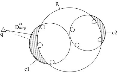
Figure 3 gives a good example. There are 3 nodes p, c1 and c2. c1 and c2 are p’s children.
Dminp c1 00000000000 00000000000 00000000000 00000000000 00000000000 00000000000 00000000000 00000000000 00000000000 00000000000 00000000000 00000000000 00000000000 00000000000 00000000000 00000000000 00000000000 00000000000 00000000000 00000000000 00000000000 11111111111 11111111111 11111111111 11111111111 11111111111 11111111111 11111111111 11111111111 11111111111 11111111111 11111111111 11111111111 11111111111 11111111111 11111111111 11111111111 11111111111 11111111111 11111111111 11111111111 11111111111 000000000 000000000 000000000 000000000 000000000 000000000 000000000 000000000 000000000 000000000 000000000 000000000 000000000 000000000 000000000 000000000 000000000 111111111 111111111 111111111 111111111 111111111 111111111 111111111 111111111 111111111 111111111 111111111 111111111 111111111 111111111 111111111 111111111 111111111 000000 000000 000000 000000 000000 111111 111111 111111 111111 111111 p c2 c1 q
Figure 3: An example to illustrate how to compute DNodeminp
which is the dotted line in the figure, but Dc1minp can be further bounded by Dminpp , since it is impossible for any point to be in the shaded area. Similarly, we get the equation for Dc1maxp.
DNodeminp and DNodemaxpare used to estimate the counts array (n,C). Again we take advantage of the triangle inequality of ball-tree. For any Node, if there exists an i (i∈[1,n]), such that
Distsi−1≤DNodemaxp<Distsi, then for∀x∈Points(Node), Distsi−1≤|x−q|<Distsi.
Accord-ing to the definition of C, we can add|Points(Node)|to Ci,Ci+1, ...Cn. The function of DNodeminp
similar to KNS1, is used to help prune uninteresting nodes.
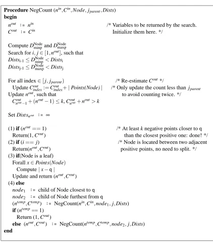
Step 2 of KNS2 is implemented by the recursive function below:
(nout,Cout) =NegCount(nin,Cin,Node,jparent,Dists)
See Figure 4 for the detailed implementation of NegCount.
Assume that on entry (nin,Cin) summarize interesting negative points for pointset V , where V is
the set of points visited so far during the search. This algorithm efficiently ensures that, on exit, (nout,Cout) summarize interesting negative points for V∪Points(Node). In addition, j
parent is a
temporary variable used to prevent multiple counts for the same point. This variable relates to the implementation of KNS2, and we do not want to go into the details in this paper.
We can stop the procedure when nout becomes 1 (which means all the k nearest neighbors of q
are in the negative class) or when we run out of nodes. noutrepresents the number of positive points in the k nearest neighbors ofq.The top-level call is
NegCount(k,C0,NegTree.Root,k+1,Dists)
where C0is an array of zeroes and Dists are defined in step 2 and obtained by applying KNS1 to the
Postree.
There are at least two situations where this algorithm can run faster than simply finding k-NN . First of all, when n=1, we can stop and exit, since this means we have found at least k negative points closer than the nearest positive neighbor to q. Notice that the k negative points we have
Procedure NegCount (nin,Cin,Node,jparent,Dists)
begin
nout := nin /* Variables to be returned by the search.
Cout := Cin Initialize them here. */
Compute DNodeminpand DNodemaxp Search for i,j∈[1,nout], such that Distsi-1≤DNodeminp <Distsi
Distsj-1≤DNodemaxp<Distsj
For all index∈[j,jparent) /* Re-estimate Cout*/
Update Cindexout :=Coutindex+|Points(Node)| /* Only update the count less than jparent
Update nout, such that to avoid counting twice. */
Cnoutout−1+ (nout−1)≤k, Cnoutout+nout>k
Set Distsnout := ∞
(1) if (nout==1) /* At least k negative points closer toq
Return(1, Cout) than the closest positive one: done! */ (2) if (i== j) /* Node is located between two adjacent
Return(nout,Cout) positive points, no need to split. */
(3) if(Node is a leaf) Forall x∈Points(Node)
Compute|x−q|
Update and return (nout,Cout)
(4) else
node1 := child of Node closest toq node2 := child of Node furthest fromq
(ntemp,Ctemp) := NegCount(nin,Cin,node
1,j,Dists)
if (ntemp== 1) Return (1, Cout)
else (nout,Cout) := NegCount(ntemp,Ctemp,node
2,j,Dists)
end
Figure 4: Procedure NegCount.
our question. This situation happens frequently for skewed data sets. The second situation is as follows: A Node can also be pruned if it is located exactly between two adjacent positive points, or it is farther away than the nthpositive point. This is because that in these situations, there is no need
to figure out which negative point is closer within the Node. Especially as n gets smaller, we have more chance to prune a node, because Distsnin decreases as nindecreases.
builds two trees, one for each class. For consistency, let’s still call them Postree and Negtree. KNSV first searches the tree whose center of gravity is closer toq. Without loses of generality, we assume Negtree is closer, so KNSV will search Negtree first. Instead of fully exploring the tree, it does a
greedy depth first search only to find k candidate points. Then KNSV moves on to search Postree. The search is the same as conventional ball-tree search (KNS1), except that it uses the kthcandidate negative point to bound the distance. After the search of Postree is done. KNSV counts how many of the k nearest neighbors so far are from the negative class. If the number is more than k/2, the al-gorithm stops. Otherwise, KNSV will go back to search Negtree for the second time, this time fully search the tree. KNSV has advantages and disadvantages. The first advantage is that it is simple, and thus it is easy to extend to many-class case. Also if the first guess of KNSV is correct and the
k candidate points are good enough to prune away many nodes, it will be faster than conventional
ball-tree search. But there are some obvious drawbacks of the algorithm. First, the guess of the winner class is only based on which class’s center of gravity is the closest toq. Notice that this is
a pure heuristic, and the probability of making a mistake is high. Second, using a greedy search to find the k candidate nearest neighbors has a high risk, since these candidates might not even be close to the true nearest neighbors. In that case, the chance for pruning away nodes from the other class becomes much smaller. We can imagine that in many situations, KNSV will end up searching the first tree for yet another time. Finally, we want to point out that KNSV claims it can perform well for many-class nearest neighbors, but this is based on the assumption that the winner class contains at least k/2 points within the nearest neighbors, which is often not true for the many-class case. Comparing to KNSV, KNS2’s advantages are (i) it uses the skewness property of a data set, which can be robustly detected before the search, and (ii) more careful design gives KNS2 more chance to speedup the search.
5. KNS3: Are at Least t of the k Nearest Neighbors Positive?
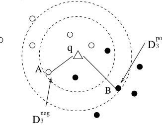
In this paper’s second new algorithm, we remove KNS2’s constraint of an assumed skewness in the class distribution. Instead, we answer a weaker question: “are at least t of the k nearest neighbors positive?”, where the questioner must supply t and k. In the usual k-NN rule, t represents a majority with respect to k, but here we consider the slightly more general form which might be used for example during classification with known false positive and false negative costs.
In KNS3, we define two important quantities:
Dtpos = distance o f the tthnearest positive neighbor o f q (8) Dnegm = distance o f the mthnearest negative neighbor o f q (9)
where m+t=k+1.
Before introducing the algorithm, we state and prove an important proposition, which relate the two quantities Dtposand Dnegm with the answer to KNS3.
Proof:
If Dtpos≤Dnegm , then there are at least t positive points closer than the mthnegative point toq. This
also implies that if we draw a ball centered atq, and with its radius equal to Dnegm , then there are
exactly m negative points and at least t positive points within the ball. Since t+m=k+1, if we use Dkto denote the distance of the kthnearest neighbor, we get Dk≤Dnegm , which means that there
are at most m−1 of the k nearest neighbors of q from the negative class. It is equivalent to say
that there are at least t of the k nearest neighbors of q are from the positive class. On the other
hand, if there are at least t of the k nearest neighbors from the positive class, then Dtpos≤Dk, the
number of negative points is at most k−t<m, so Dk≤Dnegm . This implies that Dtpos≤D neg
m is true.
Figure 5 provides an illustration. In this example, k=5,t=3. We use black dots to represent positive points, and white dots to represent negative points. The reason to redefine the problem of
D3 neg
D3 pos
q
A
B
Figure 5: An example of Dtposand Dnegm
KNS3 is to transform a k nearest neighbor searching problem to a much simpler counting prob-lem. In fact, in order to answer the question, we do not even have to compute the exact value of
Dtpos and D neg
m , instead, we can estimate them. We define Lo(Dtpos) and U p(D pos
t ) as the lower
and upper bounds of Dtpos, and similarly we define Lo(Dnegm )and U p(Dnegm )as the lower and upper
bounds of Dnegm . If at any point, U p(Dtpos)≤Lo(D neg
m ), we know Dtpos≤D neg
m , on the other hand, if U p(Dnegm )≤Lo(Dtpos), we know D
neg
m ≤Dtpos.
Now our computational task is to efficiently estimate Lo(Dtpos), U p(Dtpos), Lo(Dnegm )and U p(Dnegm ).
And it is very convenient for a ball-tree structure to do so. Below is the detailed description:
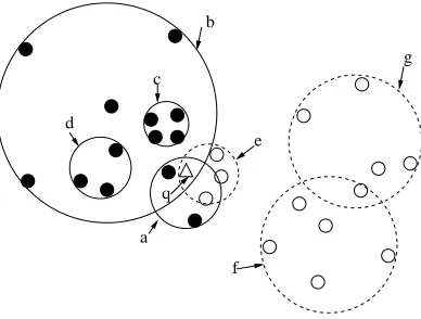
At each stage of KNS3 we have two sets of balls in use called P and N, where P is a set of balls from
Postree built from positive data points, and N consists of balls from Negtree built from negative data
points.
Both sets have the property that if a ball is in the set, then neither its ball-tree ancestors nor de-scendants are in the set, so that each point in the training set is a member of one or zero balls in
P∪N. Initially, P={PosTree.root}and N={NegTree.root}. Each stage of KNS3 analyzes P to estimate Lo(Dtpos), U p(Dtpos), and analyzes N to estimate Lo(Dnegm ), U p(Dnegm ). If possible, KNS3
involved are labeled a through g and we have
P={a,b,c,d}
N={e,f,g}
Notice that although c and d are inside b, they are not descendants of b. This is possible because when a ball is splitted, we only require the pointset of its children be disjoint, but the balls covering the children node may be overlapped.
a b
c
d
f
g
e
q
Figure 6: A configuration at the start of a stage.
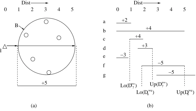
In order to compute Lo(Dtpos), we need to sort the balls u∈P, such that
∀ui,uj∈P,i< j⇒Diminp≤D j minp
Then
Lo(Dtpos) =D uj
minp, where j−1
∑
i=1|Points(ui)|<t and j
∑
i=1|Points(ui)|≥t
Symmetrically, in order to compute U p(Dtpos), we sort u∈P, such that
∀ui,uj∈P,i< j⇒Dimaxp≤Dmaxpj .
Then
U p(Dtpos) =D uj
maxp, where j−1
∑
i=1|Points(ui)|<t and j
∑
i=1|Points(ui)|≥t
Similarly, we can compute Lo(Dnegm )and U p(Dnegm ).
any location in b toqlies in the range[0,5]. The value of Lo(Dtpos)can be understood as the answer
to the following question: what if we tried to slide all the positive points within their bounds as far to the left as possible, where would the tth closest positive point lie? Similarly, we can estimate
U p(Dtpos)by sliding all the positive points to the right ends within their bounds.
Dist
0 1 2 3 4 5
Dist
0 1 2 3 4 5
Up(D6neg
)
Lo(D )7
pos
Lo(D6neg
)
Up(D )7
pos
q
+5
a +2
b +4
+4 c
d e
f
g −3
+3
−5
−5 B
(a) (b)
Figure 7: (a) The interval representation of a ball B. (b) The interval representation of the configu-ration in Figure 6
.
For example, in Figure 6, let k=12 and t=7. Then m=12−7+1=6. We can estimate (Lo(D7pos),
U p(D7pos)) and (Lo(Dneg6 ), U p(Dneg6 )), and the results are shown in Figure 5. Since the two intervals (Lo(D7pos), U p(D7pos)) and (Lo(Dneg6 ),U p(Dneg6 )) have overlap now, no conclusion can be made at this stage. Further splitting needs to be done to refine the estimation.
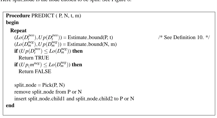
Below is the pseudo code of KNS3 algorithm: We define a loop procedure called PREDICT with the following input and output.
Answer=PREDICT(P,N,t,m)
The Answer, a boolean value, is TRUE, if there are at least t of the k nearest neighbors from the positive class; and False otherwise. Initially, P = {PosTree.root} and N = {NegTree.root}. The threshold t is given, and m=k−t+1.
Before we describe the algorithm, we first introduce two definitions. Define:
(Lo(DSi),U p(DSi)) =Estimate bound(S,i) (10)
Here S is either set P or N, and we are interested in the ith nearest neighbor of qfrom set S. The
output is the lower and upper bounds. The concrete procedure for estimating the bounds was just described.
and will not give us enough information to answer the question. In this case, we will need to split a ball-tree node and re-estimate the bounds. With more and more nodes being splitted, our estimation becomes more and more precise, and the procedure can be stopped as soon as U p(Dtpos)≤Lo(Dnegm )
or U p(Dnegm )≤Lo(Dtpos). The function of Pick(P,N)below is to choose one node either from P or
N to split. There are different strategies for picking a node, for simplicity, our implementation only randomly pick a node to split.
Define:
split node=Pick(P,N) (11)
Here split node is the node chosen to be split. See Figure 8.
Procedure PREDICT ( P, N, t, m) begin
Repeat
(Lo(Dtpos),U p(Dtpos)) = Estimate bound(P, t) /* See Definition 10. */
(Lo(Dnegm ),U p(Dnegm )) = Estimate bound(N, m)
if (U p(Dtpos)≤Lo(D neg m )) then
Return TRUE
if (U p(mneg)≤Lo(Dnegm )) then
Return FALSE
split node = Pick(P, N) remove split node from P or N
insert split node.child1 and split node.child2 to P or N
end
Figure 8: Procedure PREDICT. .
Our explanation of KNS3 was simplified for clarity. In order to avoid frequent searches over the full lengths of sets N and P, they are represented as priority queues. Each set in fact uses two queues: one prioritized by Dumaxpand the other by Duminp.This ensures that the costs of all argmins, deletions and splits are logarithmic in the queue size.
6. Experimental Results
To evaluate our algorithms, we used both real data sets (from UCI and KDD repositories) and also synthetic data sets designed to exercise the algorithms in various ways.
6.1 Synthetic Data Sets
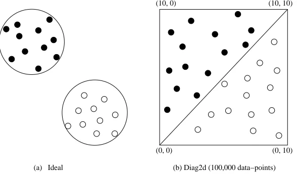
We have six synthetic data sets. The first synthetic data set we have is calledIdeal, as illustrated in Figure 6.1(a). All the data in the left upper area are assigned to the positive class, and all the data in the right lower area are assigned to the negative class. The second data set we have is calledDiag2d, as illustrated in Figure 6.1(b). The data are uniformly distributed in a 10 by 10 square. The data above the diagonal are assigned to the positive class, below diagonal are assigned to the negative class. We made several variants of Diag2d to test the robustness of KNS3. Diag2d(10%)has 10% data of Diag2d. Diag3d is a cube with uniformly distributed data and classified by a diagonal-plane. Diag10dis a 10 dimensional hypercube with uniformly distributed data and classified by a hyper-diagonal-plane. Noise-diag2dhas the same data asDiag2d(10%), but 1% of the data was assigned to the wrong class.
(10, 0)
(0, 0) (0, 10)
(10, 10)
(b) Diag2d (100,000 data−points) (a) Ideal
Figure 9: Synthetic Data Sets
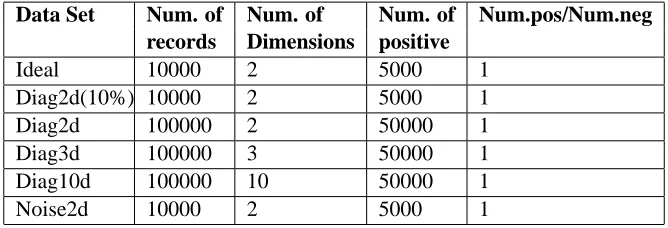
Table6.1 is a summary of the data sets in the empirical analysis.
6.2 Real-World Data Sets
We used UCI & KDD data (listed in Table 6.2), but we also experimented with data sets of particular current interest within our laboratory.
Life Sciences. These were proprietary data sets (ds1 and ds2) similar to the publicly available Open
Compound Database provided by the National Cancer Institute (NCI Open Compound Database, 2000). The two data sets are sparse. We also present results on data sets derived from ds1, denoted
Data Set Num. of Num. of Num. of Num.pos/Num.neg records Dimensions positive
Ideal 10000 2 5000 1
Diag2d(10%) 10000 2 5000 1 Diag2d 100000 2 50000 1 Diag3d 100000 3 50000 1 Diag10d 100000 10 50000 1 Noise2d 10000 2 5000 1
Table 1: Synthetic Data Sets
(PCA).
Link Detection. The first, Citeseer, is derived from the Citeseer web site (Citeseer,2002) and lists
the names of collaborators on published materials. The goal is to predict whether J Lee (the most common name) was a collaborator for each work based on who else is listed for that work. We use J Lee.100pca to represent the linear projection of the data to 100 dimensions using PCA. The second link detection data set is derived from the Internet Movie Database (IMDB, 2002) and is denoted imdb using a similar approach, but to predict the participation of Mel Blanc (again the most common participant).
UCI/KDD data. We use four large data sets from KDD/UCI repository (Bay, 1999). The data
sets can be identified from their names. They were converted to binary classification problems. Each categorical input attribute was converted into n binary attributes by a 1-of-n encoding (where
n is the number of possible values of the attribute).
1. Letter originally had 26 classes: A-Z. We performed binary classification using the letter A as the positive class and “Not A” as negative.
2. Ipums (from ipums.la.97). We predict farm status, which is binary.
3. Movie is a data set from (informedia digital video library project, 2001). The TREC-2001 Video Track organized by NIST shot boundary Task. 4 hours of video or 13 MPEG-1 video files at slightly over 2GB of data.
4. Kdd99(10%) has a binary prediction: Normal vs. Attack.
6.3 Methodology
The data set ds2 is particular interesting, because its dimension is 1.1×10⁶. Our first experiment
Data Set Num. of Num. of Num.of Num.pos/Num.neg records Dimensions positive
ds1 26733 6348 804 0.03 ds1.10pca 26733 10 804 0.03 ds1.100pca 26733 100 804 0.03 ds2 88358 1.1×10⁶ 211 0.002 ds2.100anchor 88358 100 211 0.002 J Lee.100pca 181395 100 299 0.0017 Blanc Mel 186414 10 824 0.004
Data Set Num. Num. of Num.of Num.pos/Num.neg
records Dimensions positive
Letter 20000 16 790 0.04 Ipums 70187 60 119 0.0017 Movie 38943 62 7620 0.24 Kdd99( 10% ) 494021 176 97278 0.24
Table 2: Real Data Sets
For our second set of experiments, we did 10-fold cross-validation on all the data sets. For each data set, we tested k=9 and k=101, in order to show the effect of a small value and a large value. For KNS3, we used t =⌈k/2⌉: a data point is classified as positive iff the majority of its
k nearest neighbors are positive. Since we use cross-validation, thus each experiment required R k-NN classification queries (where R is the umber of records in the data set) and each query
in-volved the k-NN among 0.9R records. A naive implementation with no ball trees would thus require 0.9R2 distance computations. We want to emphasize here that these algorithms are all exact. No
approximations were used in the classifications.
6.4 Results
Figure 10 shows the histograms of times and speed-ups for queries on the ds2 data set. For Naive
k-NN , all the queries take 87372 distance computations. For KNS1, all the queries take more than
1.0×10⁴ distance computations, (the average number of distances computed is 1.3×10⁵) which is greater than 87372 and thus traditional ball-tree search is worse than “naive” linear scan. For KNS2, most of the queries take less than 4.0×10⁴distance computations, a few points take longer time. The average number of distances computed is 6233. For KNS3, all the queries take less than 1.0×10⁴ distance computations, the average number of distances computed is 3411. The lower
three figures illustrate speed-up achieved for KNS1, KNS2 and KNS3 over naive linear scan. The figures show the distribution of the speedup obtained for each query. From 10(d) we can see that on average, KNS1 is even slower than the naive algorithm. KNS2 can get from 2- to 250-fold speedups. On average, it has a 14-fold speedup. KNS3 can get from 2- to 2500-fold speedups. On average, it has a 26-fold speedups.
kns1
distance computation
number of data
0 20000 40000 60000 80000 120000
0 100 200 300 400 500 kns2 distance computation
number of data
0 20000 40000 60000 80000 120000
0 100 200 300 400 500 kns3 distance computation
number of data
0 20000 40000 60000 80000 120000
0 100 200 300 400 500 kns1 speedup
folds of speed up
number of data
0 20 40 60 80 100
0 200 400 600 800 kns2 speedup
folds of speed up
number of data
0 20 40 60 80 100
0 200 400 600 800 kns3 speedup
folds of speed up
number of data
0 20 40 60 80 100
0
200
400
600
800
Figure 10: (a) Distribution of times taken for queries of KNS1 (b) Distribution of times taken for queries of KNS2 (c) Distribution of times taken for queries of KNS3 (d) Distribution of speedup for queries achieved for KNS1 (e) Distribution of speedup for queries achieved for KNS2 (f) Distribution of speedup for queries achieved for KNS3
time on an unloaded 2 GHz Pentium. We then examine the speedups of KNS1 (traditional use of a ball-tree) and our two new ball-tree methods (KNS2 and KNS3). Generally speaking, the speedup achieved for distance computations on all three algorithms are greater than the correspond-ing speedup for wall-clock time. This is expected, because the wall-clock time also includes the time for building ball trees, generating priority queues and searching. We can see that for the syn-thetic data sets, KNS1 and KNS2 yield 2-700 fold speedup over naive. KNS3 yields a 2-4500 fold speedup. Notice that KNS2 can’t beat KNS1 for these data sets, because KNS2 is designed to speedup k-NN search on data sets with unbalanced output classes. Since all the synthetic data sets have equal number of data from positive and negative classes, KNS2 has no advantage.
over naive. KNS2 and KNS3 do, however, and in some cases they are hundreds of times faster than KNS1.
NAIVE KNS1 KNS2 KNS3
dists time dists time dists time dists time (secs) speedup speedup speedup speedup speedup speedup ideal k=9 9.0×10⁷ 30 96.7 56.5 112.9 78.5 4500 486
k=101 23.0 10.2 24.7 14.7 4500 432
Diag2d(10%)k=9 9.0×10⁷ 30 91 51.1 88.2 52.4 282 27.1
k=101 22.3 8.7 21.3 9.3 167.9 15.9
Diag2d k=9 9.0×10⁹ 3440 738 366 664 372 2593 287
k=101 202.9 104 191 107.5 2062 287
Diag3d k=9 9.0×10⁹ 4060 361 184.5 296 184.5 1049 176.5
k=101 111 56.4 95.6 48.9 585 78.1
Diag10d k=9 9.0×10⁹ 6080 7.1 5.3 7.3 5.2 12.7 2.2
k=101 3.3 2.5 3.1 1.9 6.1 0.7
Noise2d k=9 9.0×10⁷ 40 91.8 20.1 79.6 30.1 142 42.7
k=101 22.3 4 16.7 4.5 94.7 43.5
ds1 k=9 6.4×10⁸ 4830 1.6 1.0 4.7 3.1 12.8 5.8
k=101 1.0 0.7 1.6 1.1 10 4.2
ds1.10pca k=9 6.4×10⁸ 420 11.8 11.0 33.6 21.4 71 20
k=101 4.6 3.4 6.5 4.0 40 6.1
ds1.100pca k=9 6.4×10⁸ 2190 1.7 1.8 7.6 7.4 23.7 29.6
k=101 0.97 1.0 1.6 1.6 16.4 6.8
ds2 k=9 8.5×10⁹ 105500 0.64 0.24 14.0 2.8 25.6 3.0
k=101 0.61 0.24 2.4 0.83 28.7 3.3
ds2.100- k=9 7.0×10⁹ 24210 15.8 14.3 185.3 144 580 311
k=101 10.9 14.3 23.0 19.4 612 248
J Lee.100- k=9 3.6×10¹⁰ 142000 2.6 2.4 28.4 27.2 15.6 12.6
k=101 2.2 1.9 12.6 11.6 37.4 27.2
Blanc Mel k=9 3.8×10¹⁰ 44300 3.0 3.0 47.5 60.8 51.9 60.7
k=101 2.9 3.1 7.1 33 203 134.0
Letter k=9 3.6×10⁸ 290 8.5 7.1 42.9 26.4 94.2 25.5
k=101 3.5 2.6 9.0 5.7 45.9 9.4
Ipums k=9 4.4×10⁹ 9520 195 136 665 501 1003 515
k=101 69.1 50.4 144.6 121 5264 544
Movie k=9 1.4×10⁹ 3100 16.1 13.8 29.8 24.8 50.5 22.4
k=101 9.1 7.7 10.5 8.1 33.3 11.6
Kddcup99 k=9 2.7×10¹¹ 1670000 4.2 4.2 574 702 4 4.1
(10%) k=101 4.2 4.2 187.7 226.2 3.9 3.9
Table 3: Number of distance computations and wall-clock-time for Naive k-NN classification (2nd column). Acceleration for normal use of KNS1 (in terms of num. distances and time). Accelerations of new methods KNS2 and KNS3 in other columns. Naive times are inde-pendent of k.
7. Comments and Related Work
Why k-NN ? k-NN is an old classification method, often not achieving the highest possible
accu-racies when compared to more complex methods. Why study it? There are many reasons. k-NN is a useful sanity check or baseline against which to check more sophisticated algorithms provided
k-NN is tractable. It is often the first line of attack in a new complex problem due to its
theo-retical properties, which explains its surprisingly good performance in practice in many cases. For these reason and others, k-NN is still popular in some fields that need classification, for example Computer Vision and QSAR analysis of High Throughput Screening data (e.g., Zheng and Tropsha, 2000). Finally, we believe that the same insights that accelerate k-NN will apply to more modern algorithms. From a theoretical viewpoint, many classification algorithms can be viewed simply as the nearest-neighbor method with a certain broader notion of distance function; see for example Baxter and Bartlett (1998) for such a broad notion. RKHS kernel methods use another example of a broadened notion of distance function. More concretely, we have applied similar ideas to speed up nonparametric Bayes classifiers, in work to be submitted.
Applicability of other proximity query work. For the problem of “find the k nearest datapoints”
(as opposed to our question of “perform k-NN or Kernel classification”) in high dimensions, the fre-quent failure of a traditional ball-tree to beat naive has lead to some very ingenious and innovative alternatives, based on random projections, hashing discretized cubes, and acceptance of approxi-mate answers. For example Gionis et al. (1999) gives a hashing method that was demonstrated to provide speedups over a ball-tree-based approach in 64 dimensions by a factor of 2-5 depending on how much error in the approximate answer was permitted. Another approximate k-NN idea is in Arya et al. (1998), one of the first k-NN approaches to use a priority queue of nodes, in this case achieving a 3-fold speedup with an approximation to the true k-NN . In (Liu et al., 2004a), we introduced a variant of ball-tree structures which allow non-backtracking search to speed up approximate nearest neighbor, and we observed up to 700-fold accelerations over conventional ball-tree based k-NN . Similar idea has been proposed by Indyk (2001). However, these approaches are based on the notion that any points falling within a factor of(1+ε)times the true nearest neighbor distance are acceptable substitutes for the true nearest neighbor. Noting in particular that distances in high-dimensional spaces tend to occupy a decreasing range of continuous values (Hammersley, 1950), it remains unclear whether schemes based upon the absolute values of the distances rather than their ranks are relevant to the classification task. Our approach, because it need not find the
k-NN to answer the relevant statistical question, finds an answer without approximation. The fact
that our methods are easily modified to allow (1+ε)approximation in the manner of Arya et al. (1998) suggests an obvious avenue for future research.
No free lunch. For uniform high-dimensional data no amount of trickery can save us. The
expla-nation for the promising empirical results is that all the inter-dependences in the data mean we are working in a space of much lower intrinsic dimensionality (Maneewongvatana and Mount, 2001). Note though, that in experiments not reported here, QSAR and vision k-NN classifiers give better performance on the original data than on PCA-projected low dimensional data, indicating that some of these dependencies are non-linear.
Summary. This paper has introduced and evaluated two new algorithms for more effectively
References
S. Arya, D. M. Mount, N. S. Netanyahu, R. Silverman, and A. Y. Wu. An optimal algorithm for approximate nearest neighbor searching fixed dimensions. Journal of the ACM, 45(6):891–923, 1998. URLciteseer.ist.psu.edu/arya94optimal.html.
J. Baxter and P. Bartlett. The Canonical Distortion Measure in Feature Space and 1-NN Classifica-tion. In Advances in Neural Information Processing Systems 10. Morgan Kaufmann, 1998.
S. D. Bay. UCI KDD Archive [http://kdd.ics.uci.edu]. Irvine, CA: University of California, Dept of Information and Computer Science, 1999.
C. Cardie and N. Howe. Improving minority class prediction using case-specific feature weights. In Proceedings of 14th International Conference on Machine Learning, pages 57–65. Morgan Kaufmann, 1997. URLciteseer.nj.nec.com/cardie97improving.html.
C. L. Chang. Finding prototypes for nearest neighbor classifiers. IEEE Trans. Computers, C-23 (11):1179–1184, November 1974.
P. Ciaccia, M. Patella, and P. Zezula. M-tree: An efficient access method for similarity search in metric spaces. In Proceedings of the 23rd VLDB International Conference, September 1997.
K. Clarkson. Nearest Neighbor Searching in Metric Spaces: Experimental Results for sb(S). , 2002.
S. Cost and S. Salzberg. A Weighted Nearest Neighbour Algorithm for Learning with Symbolic Features. Machine Learning, 10:57–67, 1993.
T. M. Cover and P. E. Hart. Nearest neighbor pattern classification. IEEE Trans. Information Theory, IT-13,no.1:21–27, 1967.
S. C. Deerwester, S. T. Dumais, T. K. Landauer, G. W. Furnas, and R. A. Harshman. Indexing by latent semantic analysis. Journal of the American Society of Information Science, 41(6):391–407, 1990.
K. Deng and A. W. Moore. Multiresolution Instance-based Learning. In Proceedings of the Twelfth
International Joint Conference on Artificial Intelligence, pages 1233–1239, San Francisco, 1995.
Morgan Kaufmann.
L. Devroye and T. J. Wagner. Nearest neighbor methods in discrimination, volume 2. P.R. Krish-naiah and L. N. Kanal, eds., North-Holland, 1982.
A. Djouadi and E. Bouktache. A fast algorithm for the nearest-neighbor classifier. IEEE Trans.
Pattern Analysis and Machine Intelligence, 19(3):277–282, March 1997.
N. R. Draper and H. Smith. Applied Regression Analysis, 2nd ed. John Wiley, New York, 1981.
R. O. Duda and P. E. Hart. Pattern Classification and Scene Analysis. John Wiley & Sons, 1973.
C. Faloutsos, R. Barber, M. Flickner, J. Hafner, W. Niblack, D. Petkovic, and William Equitz. Efficient and effective querying by image content. Journal of Intelligent Information Systems, 3 (3/4):231–262, 1994.
T. Fawcett and F. J. Provost. Adaptive fraud detection. Data Mining and Knowledge Discovery, 1 (3):291–316, 1997. URLciteseer.nj.nec.com/fawcett97adaptive.html.
F. P. Fisher and E. A. Patrick. A preprocessing algorithm for nearest neighbor decision rules. In
Proc. Nat’l Electronic Conf., volume 26, pages 481–485, December 1970.
M. Flickner, H. Sawhney, W. Niblack, J. Ashley, Q. Huang, B. Dom, M. Gorkani, J. Hafner, D. Lee, D. Petkovic, D. Steele, and P. Yanker. Query by image and video content: the qbic system. IEEE
Computer, 28:23–32, 1995.
J. H. Friedman, J. L. Bentley, and R. A. Finkel. An algorithm for finding best matches in logarithmic expected time. ACM Transactions on Mathematical Software, 3(3):209–226, September 1977.
K. Fukunaga and P.M. Narendra. A Branch and Bound Algorithm for Computing K-Nearest Neigh-bors. IEEE Trans. Computers, C-24(7):750–753, 1975.
G. W. Gates. The reduced nearest neighbor rule. IEEE Trans. Information Theory, IT-18(5):431– 433, May 1972.
A. Gionis, P. Indyk, and R. Motwani. Similarity Search in High Dimensions via Hashing. In
Proceedings of the 25th VLDB Conference, 1999.
A. Gray and A. W. Moore. N-Body Problems in Statistical Learning. In Todd K. Leen, Thomas G. Dietterich, and Volker Tresp, editors, Advances in Neural Information Processing Systems 13. MIT Press, 2001.
A. Guttman. R-trees: A dynamic index structure for spatial searching. In Proceedings of the Third
ACM SIGACT-SIGMOD Symposium on Principles of Database Systems. Assn for Computing
Machinery, April 1984.
J. M. Hammersley. The Distribution of Distances in a Hypersphere. Annals of Mathematical
Statis-tics, 21:447–452, 1950.
P. E. Hart. The condensed nearest neighbor rule. IEEE Trans. Information Theory, IT-14(5):515– 516, May 1968.
T. Hastie and R. Tibshirani. Discriminant adaptive nearest neighbor classification. IEEE Trans.
Pattern Analysis and Machine Intelligence, 18(6):607–615, June 1996.
P. Indyk. On approximate nearest neighbors under l∞ norm. Journal of Computer and System
Sciences, 63(4), 2001.
CMU informedia digital video library project. The trec-2001 video trackorganized by nist shot boundary task, 2001.
V. Koivune and S. Kassam. Nearest neighbor filters for multivariate data. In IEEE Workshop on
P. Komarek and A. W. Moore. Fast robust logistic regression for large sparse datasets with binary outputs. In Artificial Intelligence and Statistics, 2003.
C. Kruegel and G. Vigna. Anomaly detection of web-based attacks. In Proceedings of the 10th
ACM conference on Computer and communications security table of contents, pages 251–261,
2003.
E. Lee and S. Chae. Fast design of reduced-complexity nearest-neighbor classifiers using triangular inequality. IEEE Trans. Pattern Analysis and Machine Intelligence, 20(5):562–566, May 1998.
T. Liu, A. W. Moore, A. Gray, and K. Yang. An investigation of practical approximate nearest neighbor algorithms. In Proceedings of Neural Information Processing Systems, 2004a.
T. Liu, K. Yang, and A. Moore. The ioc algorithm: Efficient many-class non-parametric classifi-cation for high-dimensional data. In Proceedings of the conference on Knowledge Discovery in
Databases (KDD), 2004b.
S. Maneewongvatana and D. M. Mount. The analysis of a probabilistic approach to nearest neighbor searching. In In Proceedings of WADS 2001, 2001.
A. W. Moore. The Anchors Hierarchy: Using the Triangle Inequality to Survive High-Dimensional Data. In Twelfth Conference on Uncertainty in Artificial Intelligence. AAAI Press, 2000.
S. Omachi and H. Aso. A fast algorithm for a k-nn classifier based on branch and bound method and computational quantity estimation. In In Systems and Computers in Japan, vol.31, no.6, pp.1-9, 2000.
S. M. Omohundro. Bumptrees for Efficient Function, Constraint, and Classification Learning. In R. P. Lippmann, J. E. Moody, and D. S. Touretzky, editors, Advances in Neural Information
Processing Systems 3. Morgan Kaufmann, 1991.
S. M. Omohundro. Efficient Algorithms with Neural Network Behaviour. Journal of Complex
Systems, 1(2):273–347, 1987.
A. M. Palau and R. R. Snapp. The labeled cell classifier: A fast approximation to k nearest neigh-bors. In Proceedings of the 14th International Conference on Pattern Recognition, 1998.
E. P. D. Pednault, B. K. Rosen, and C. Apte. Handling imbalanced data sets in insurance risk modeling, 2000.
D. Pelleg and A. W. Moore. Accelerating Exact k-means Algorithms with Geometric Reasoning. In Proceedings of the Fifth International Conference on Knowledge Discovery and Data Mining. ACM, 1999.
A. Pentland, R. Picard, and S. Sclaroff. Photobook: Content-based manipulation of image databases, 1994. URLciteseer.ist.psu.edu/pentland95photobook.html.
F. P. Preparata and M. Shamos. Computational Geometry. Springer-Verlag, 1985.
Y. Qi, A. Hauptman, and T. Liu. Supervised classification for video shot segmentation. In
G. L. Ritter, H. B. Woodruff, S. R. Lowry, and T. L. Isenhour. An algorithm for a selective nearest neighbor decision rule. IEEE Trans. Information Theory, IT-21(11):665–669, November 1975.
G. Salton and M. McGill. Introduction to Modern Information Retrieval. McGraw-Hill Book Company, New York, NY, 1983.
I. K. Sethi. A fast algorithm for recognizing nearest neighbors. IEEE Trans. Systems, Man, and
Cybernetics, SMC-11(3):245–248, March 1981.
A. Smeulders and R. Jain, editors. Image Databases and Multi-media Search. World Scientific Publishing Company, 1996.
S. Stolfo, W. Fan, W. Lee, A. Prodromidis, and P. Chan. Credit card fraud detection using meta-learning: Issues and initial results, 1997. URLciteseer.nj.nec.com/stolfo97credit.html.
Y. Hamamoto S. Uchimura and S. Tomita. A bootstrap technique for nearest neighbor classifier design. IEEE Trans. Pattern Analysis and Machine Intelligence, 19(1):73–79, 1997.
J. K. Uhlmann. Satisfying general proximity/similarity queries with metric trees. Information
Processing Letters, 40:175–179, 1991.
K. Woods, K. Bowyer, and W. P. Kegelmeyer Jr. Combination of multiple classifiers using local accuracy estimates. IEEE Trans. Pattern Analysis and Machine Intelligence, 19(4):405–410, 1997.
B. Zhang and S. Srihari. Fast k-nearest neighbor classification using cluster-based trees. IEEE
Trans. Pattern Analysis and Machine Intelligence, 26(4):525–528, April 2004.
T. Zhang, R. Ramakrishnan, and M. Livny. BIRCH: An Efficient Data Clustering Method for Very Large Databases. In Proceedings of the Fifteenth ACM SIGACT-SIGMOD-SIGART Symposium
on Principles of Database Systems : PODS 1996. ACM, 1996.