Incremental Support Vector Learning:
Analysis, Implementation and Applications
Pavel Laskov [email protected]
Christian Gehl [email protected]
Stefan Kr ¨uger [email protected]
Fraunhofer-FIRST.IDA Kekul´estrasse 7 12489 Berlin, Germany
Klaus-Robert M ¨uller [email protected]
Fraunhofer-FIRST.IDA Kekul´estrasse 7 12489 Berlin, Germany and
University of Potsdam August-Bebelstrasse 89 14482 Potsdam, Germany
Editors: Kristin P. Bennett, Emilio Parrado-Hern´andez
Abstract
Incremental Support Vector Machines (SVM) are instrumental in practical applications of online learning. This work focuses on the design and analysis of efficient incremental SVM learning, with the aim of providing a fast, numerically stable and robust implementation. A detailed analysis of convergence and of algorithmic complexity of incremental SVM learning is carried out. Based on this analysis, a new design of storage and numerical operations is proposed, which speeds up the training of an incremental SVM by a factor of 5 to 20. The performance of the new algorithm is demonstrated in two scenarios: learning with limited resources and active learning. Various applications of the algorithm, such as in drug discovery, online monitoring of industrial devices and and surveillance of network traffic, can be foreseen.
Keywords: incremental SVM, online learning, drug discovery, intrusion detection
1. Introduction
Online learning is a classical learning scenario in which training data is provided one example at a time, as opposed to the batch mode in which all examples are available at once (e.g. Robbins and Munro (1951); Murata (1992); Saad (1998); Bishop (1995); Orr and M¨uller (1998); LeCun et al. (1998); Murata et al. (2002)).
that they allow to incorporate additional training data, when it is available, without re-training from scratch. Given that training is usually the most computationally intensive task, it is not surprising that availability of online algorithms is a major pre-requisite imposed by practitioners that work on large data sets (cf. LeCun et al. (1998)) or even have to perform real-time estimation tasks for con-tinuous data streams, such as in intrusion detection (e.g. Laskov et al. (2004); Eskin et al. (2002)), web-mining (e.g. Chakrabarti (2002)) or brain computer interfacing (e.g. Blankertz et al. (2003)).
In the 1980’s online algorithms were investigated in the context of PAC learning (e.g. Angluin (1988); Littlestone et al. (1991)). With the emergence of Support Vector Machines (SVM) in the mid-1990’s, interest to online algorithms for this learning method arose as well. However, early work on this subject (e.g. Syed et al., 1999; R¨uping, 2002; Kivinen et al., 2001; Ralaivola and d’Alch´e Buc, 2001) provided only approximate solutions.
An exact solution to the problem of online SVM learning has been found by Cauwenberghs and Poggio (2001). Their incremental algorithm (hereinafter referred to as a C&P algorithm) updates an optimal solution of an SVM training problem after one training example is added (or removed).
Unfortunately acceptance of the C&P algorithm in the machine learning community has been somewhat marginal, not to mention that it remains widely unknown to potential practitioners. Only a handful of follow-up publications is known that extend this algorithm to other related learning problems (e.g. Martin, 2002; Ma et al., 2003; Tax and Laskov, 2003); to our knowledge, no suc-cessful practical applications of this algorithm has been reported.
At a first glance, a limited interest to incremental SVM learning may seem to result the absence of well-accepted implementations, such as its counterparts SVMlight(Joachims, 1999), SMO (Platt, 1999) and LIBSVM (Chang and Lin, 2000) for batch SVM learning. The original Matlab imple-mentation by the authors1 has essentially the semantics of batch learning: training examples are loaded all at once (although learned one at a time) and unlearning is only used for computation of the – ingenious – leave-one-out bound.
There are, however, deeper reasons why incremental SVM may not be so easy to implement. To understand them – and to build a foundation for an efficient design and implementation of the algorithm, a detailed analysis of the incremental SVM technique is carried out in this paper. In particular we address the “accounting” details, which contain pitfalls of performance bottlenecks unless underlying data structures are carefully designed, and analyze convergence of the algorithm.
The following are the main results of our analysis:
1. Computational complexity of a minor iteration of the algorithm is quadratic in the number of training examples learned so far. The actual runtime depends on the balance of memory access and arithmetic operations in a minor iteration.
2. The main incremental step of the algorithm is guaranteed to bring progress in the objective function if a kernel matrix is positive semi-definite.
Based on the results of our analysis, we propose a new storage design and organization of computation for a minor iteration of the algorithm. The idea is to judiciously use row-major and column-major storage of matrices, instead of one-dimensional arrays, in order to possibly eliminate selection operations. The second building block of our design is gaxpy-type matrix-vector multipli-cation, which allows to further minimize selection operations which cannot be eliminated by storage
design alone. Our experiments show that the new design improves computational efficiency by the factor of 5 to 20.
To demonstrate applicability of incremental SVM to practical applications, two learning scenar-ios are presented. Learning with limited resources allows to learn from large data sets with as little as 2% of the data needed to be stored in memory. Active learning is another powerful technique by means of which learning can be efficiently carried out in large data sets with limited availability of labels. Various applications of the algorithm, such as in drug discovery, online monitoring of industrial devices and and surveillance of network traffic, can be foreseen.
In order to make this contribution self-contained, we begin with the presentation of the C&P algorithm, highlighting the details that are necessary for a subsequent analysis. An extension of the basic incremental SVM to one-class classification is presented in Section 3. Convergence analy-sis of the algorithm is carried out in Section 4. Analyanaly-sis of computational complexity, design of efficient storage and organization of operations are presented and evaluated in Section 5. Finally, potential applications of incremental SVM for learning with limited resources and active learning are illustrated in Section 6.
2. Incremental SVM Algorithm
In this section we present the basic incremental SVM algorithm. Before proceeding with our pre-sentation we need to establish some notation.
2.1 Preliminaries
We assume the training data and their labels are given by a set
{(x1,y1), . . . ,(xn,yn)}.
The inner product between data points in a feature space is defined by a kernel function k(xi,xj).
The n×n kernel matrix K0 contains the inner product values for all 1≤i,j≤n. The matrix K is
obtained from the kernel matrix by incorporating the labels:
K=K0⊙(yyT).
The operator⊙denotes the element-wise matrix product, and a vector y denotes labels as an n×1 vector. Using this notation, the SVM training problem can be formulated as
max
µ 0≤minα≤C yTα=0
W :=−1Tα+C2αTKα+µyTα. (1)
Unlike the classical setting of the SVM training problem, which is usually formulated as maximiza-tion or minimizamaximiza-tion, the problem (1) is a saddle-point formulamaximiza-tion obtained by incorporating the equality constraint directly into the cost function. The reason for such construction will become clear shortly.
2.2 Derivation of the Basic Incremental SVM Algorithm
assignment is not an optimal solution, i.e. when xc should become a support vector, the weights
of other points and the threshold µ must be updated in order to obtain an optimal solution for the enlarged data set. The procedure can be reversed for a removal of an example: its weight is forced to zero while updating weights of the remaining examples and the threshold µ so that the solution obtained with αc=0 is optimal for the reduced data set. For the remaining part of this paper we
only consider addition of examples.
The saddle point of the problem (1) is given by the Kuhn-Tucker conditions:
gi:=−1+Ki,:α+µyi
≥0, if αi=0
=0, if 0<αi<C
≤0, if αi=C
(2)
∂W
∂µ :=y
Tα=0. (3)
Before an addition of a new example xc, the Kuhn-Tucker conditions are satisfied for all previous
examples. The goal of the weight update in the incremental SVM algorithm is to find a weight assignment such that the Kuhn-Tucker conditions are satisfied for the enlarged data set.
Let us introduce some further notation. Let the set S denote unbounded support vectors (0<
αi <C), the set E denote bounded support vectors (αi =C), and the set O denote non-support
vectors (αi=0); let R=E∪O. These index sets induce respective partitions on the kernel matrix
K and the label vector y (we shall use the lower-case letters s, e, o and r for such partitions).
By writing out the Kuhn-Tucker conditions (2)–(3) before and after an update∆αwe obtain the following condition that must be satisfied after an update:
∆gc
∆gs
∆gr
0 =
yc Kcs
ys Kss
yr Krs
0 yTs ∆ µ ∆αs | {z }
∆s
+∆αc
KccT KcsT KcrT yc
. (4)
One can see that∆αcis in equilibrium with∆αsand µ: any change to∆αcmust be absorbed by the
appropriate changes in∆αsand µ in order for the condition (4) to hold.
The main equilibrium condition (4) can be further refined as follows. It follows from (2) that
∆gs=0. Then lines 2 and 4 of the system (4) can be re-written as 0 0 =
0 αTs
αs Kss
∆s+
α c
KcsT
∆αc. (5)
This linear system is easily solved for∆s as follows:
∆s =β∆αc, (6)
where
β= −
0 αTs
αs Kss −1 | {z }
Q
α c
KcsT | {z }
~η
(7)
One can further substitute (6) into lines 1 and 3 of the system (4):
∆ gc
∆gr
=γ∆αc, (8)
where
γ=
yc Kcs
yr Krs
β+
Kcc
KcrT
(9)
is the gradient of the manifold of gradients grat an optimal solution parameterized byαc.
The upshot of these derivations is that the update is controlled by very simple sensitivity rela-tions (6) and (8), whereβis sensitivity of∆s with respect to∆αc andγis sensitivity of∆gc,r with
respect to∆αc.
2.3 Accounting
Unfortunately the system (4) cannot be used directly to obtain the new SVM state. The problem lies in the changing composition of the sets S and R with the change of∆s and∆αc in Eq. (4). To
handle this problem, the main strategy of the algorithm is to identify the largest increase∆αc such
that some point migrates between the sets S and R. Four cases must be considered to account for such structural changes:
1. Someαiin S reaches a bound (an upper or a lower one). Letεbe a small number. Compute
the sets
I
+S={i∈S :βi>ε}I
−S={i∈S :βi<−ε}.The examples in set
I
+S have positive sensitivity with respect to the weight of the current example; that is, their weight would increase by taking the step∆αc.2These examples shouldbe tested for reaching the upper bound C. Likewise, the examples in set
I
−S should be tested for reaching zero. The examples with−ε<βi<εshould be ignored, as they are insensitiveto∆αc. Thus the possible weight updates are
∆αmax
i =
(
C−αi, if i∈
I
+S −αi, if i∈I
−S,and the largest possible∆αSc before some example in S moves to R is
∆αS
c=absmin
i∈IS
+∪I−S
∆αmax i
βi
, (10)
where
absmin
i (x):=mini |xi| ·sign(x(argmini
|xi|)).
2. Some gi in R reaches zero. Compute the sets
I
+R={i∈E :γi>ε}I
−R={i∈O :γi<−ε}.The examples in set
I
+Rhave positive sensitivity of the gradient with respect to the weight ofthe current example. Therefore their (negative) gradients can potentially reach zero. Likewise, gradients of the examples in set
I
−Rare positive but are pushed towards zero with the increasing weight of the current example. Thus the largest increase∆αgc before some point in R movesto S can be computed as
∆αR
c = min i∈I+R∪I−R
−gi
γi
. (11)
3. gcbecomes zero. This case is similar to case 2, with the feasibility test in the form
γc>ε.
If the update is feasible the largest step∆αgc is computed as
∆αg c=
−gc
γc
. (12)
4. αcreaches C. The largest possible increment∆ααc is clearly
∆αα
c =C−αc. (13)
Finally, the smallest of the four values
∆αmax
c =min(∆αSc,∆αcR,∆αgc,∆ααc) (14)
constitutes the largest possible increment ofαc.
After the largest possible increment ofαcis determined, the updates∆s and∆g are carried out.
The inverse matrix Q must be also re-computed in order to account for the new composition of the set S. Efficient update of this matrix is presented in section 2.4. The sensitivity vectors βandγ must be also re-computed. The process repeats until the gradient of the current example becomes zero or its weight reaches C. The high-level summary of incremental SVM algorithm is given in Algorithm 1.
2.4 Recursive Update of the Inverse Matrix
It is clearly infeasible to explicitly invert the matrix Q in Eq. (7) every time the set S is changed. Luckily, it is possible to use the fact that this set is always updated one element at a time – an example is either added to, or removed from the set S.
Consider addition first. When the example xk3is added to the set S, the matrix to be inverted is
partitioned as follows:
R :=
0 yTs yk
ys Kss KksT
yk Kks Kkk =
Q−1 ηk
ηT k Kkk
, (15)
where
ηk=
yk
KksT
.
Algorithm 1 Incremental SVM algorithm: high-level summary. 1: Read example xc, compute gc.
2: while gc<0 &αc<C do
3: Computeβandγaccording to (7), (9).
4: Compute∆αSc,∆αRc,∆αgc and∆ααc according to (10)–(13).
5: Compute∆αmaxc according to (14). 6: αc←αc+∆αmaxc .
7: αs←β∆αmaxc
8: gc,r←γ∆αmaxc
9: Let k be the index of the example yielding the minimum in (14). 10: if k∈S then
11: Move k from S to either E or O.
12: else if k∈E∪O then
13: Move k from either E or O to S.
14: else
15: {k=c: do nothing, the algorithm terminates.}
16: end if
17: Update Q recursively. {See section 2.4.}
18: end while
Defineβk=−Qηk, and denote the enlarged inverse matrix by ˜Q. Applying the
Sherman-Morrison-Woodbury formula for block matrix inversion (see e.g. Golub and van Loan (1996)) to ˜Q, we obtain:
Q−1 ηk
ηT k Kkk
−1 | {z }
˜ Q
=
Q+κ−1(Qη
k)(Qηk)T −κ−1Qηk −κ−1(Qη
k)T κ−1
=
Q+κ−1β
kβTk κ−1βk
κ−1βT
k κ−1
=
Q 0
0 0
+1
κ
β k
1
βT
k 1
, (16)
where
κ =Kkk−ηTkQηk. (17)
Thus the update of the inverse matrix involves expansion with a zero row and column and addition of a rank-one matrix obtained via a matrix-vector multiplication. The running time needed for an update of the inverse matrix is quadratic in the size of Q, which is much better than explicit inversion.
The removal case is straightforward. Knowing the inverse matrix ˜Q and using (16), we can write
˜
Q=
q11 q12 q21 q22
=
Q+κ−1β
kβTk κ−1βk
κ−1βT
k κ−1
Re-writing this block matrix expression component-wise, we have:
Q=q11−κ−1βkβTk (18)
βk=κq12=q12/q22 (19)
βT
k =κq21=q21/q22 (20)
κ−1=q
22. (21)
Substituting the last three relations into the first we obtain:
Q=q11− q12q21
q22
. (22)
The running time of the removal operations is also quadratic in the size of Q.
3. Extension to One-Class Classification
Availability of labels, especially online, may not be possible in certain applications. For example, analysis of security logs is extremely time-consuming, and labels may be available only in limited quantities after forensic investigation. As another example, monitoring of critical infrastructures, such as power lines or nuclear reactors, must prevent a system from reaching a failure state which may lead to gravest consequences. Nevertheless, algorithms similar to SVM classification can be applied for data-description, i.e. for automatic inference of a concept descriptions deviations from which are to be considered abnormal. Since examples of the class to be learned are not (or rarely) available, the problem is known as “one-class classification”.
The two well-known approaches to one-class classification are separation of data points from the origin (Sch¨olkopf et al., 2001) and spanning of data points with a sphere (Tax and Duin, 1999). Although they use different geometric constructions, these approaches lead to similar, and in certain cases even identical, formulations of dual optimization problems. As we shall see, incremental learning can be naturally extended to both of these approaches.
The dual formulation of the “sphere” one-class classification is given by the following quadratic program:
max
α n
∑
i=1
αik(xi,xi)−
1 2
n
∑
i=1 n
∑
j=1
αiαjk(xi,xj)
subject to: 0≤αi≤C,i=1, . . . ,n n
∑
i=1
αi=1.
(23)
In order to extend the C&P algorithm for this problem consider the following abstract saddle-point quadratic problem:
max
µ 0≤minα≤C aTα+b=0
W :=−cTα+C 2α
THα+µ(aTα+b). (24)
It can be easily seen that formulation (24) generalizes both problems (23) and (1), subject to follow-ing definition of the abstract parameters:
Algorithm 2 Initialization of incremental one-class SVM.
1: Take the first⌊C1⌋objects, assign them weight C and put them in E. 2: Take the next object c, assignαc=1− ⌊C1⌋C and put it in S.
3: Compute the gradients giof all objects, using Eq. (2).
4: Compute µ so as to ensure non-positive gradients in E: µ=−max
i∈E gi
5: Enter the main loop of the incremental algorithm.
The C&P algorithm presented in sections 2.2–2.4 can be applied to formulation (24) almost without modification. The only necessary adjustment is a special initialization procedure for identification of an initial feasible solution presented in Algorithm 2.4
4. Convergence Analysis
A very attractive feature of Algorithm 1 is that it obviously makes progress to an optimal solution if a non-zero update∆αcis found. Thus potential convergence problems arise only when a zero update
step is encountered. This can happen in several situations. First, if the set S is empty, no non-zero update of∆αc is possible since otherwise the equality constraint of the SVM training problem is
violated. Second, a zero update can occur when two or more points simultaneously migrate between the index sets. In this case, each subsequent point requires a structural update without improvement of∆αc. Furthermore, it must be guaranteed, that after a point migrates from one set to another,
say from E to S, it is not immediately thrown out after the structure and the sensitivity parameters are re-computed. These issues constitute the scope of convergence analysis to be covered in this section. In particular we present a technique for handling the special case of the empty set S and show that immediate cycling is impossible if a kernel matrix is positive semi-definite.
4.1 Empty Set S
The procedure presented in the previous two sections requires a non-empty set of unbounded support vectors, otherwise a zero matrix must be inverted in Eq. (7). To handle this situation, observe that the main instrument needed to derive the sensitivity relations is pegging of the gradient to zero for unbounded support vectors, which follows from the Kuhn-Ticker conditions (2). Notice that the gradient can also be zero for some points in sets E and O. Therefore, if the set S is empty we can freely move some examples with zero gradients from the sets E and O to it and continue from there. The question arises: what if no points with zero gradients can be found in E or O?
With∆α=0,∆αc=0 and no examples in the set S, the equilibrium condition (4) reduces to
∆gc=yc∆µ
∆gr=yr∆µ.
(25)
This is an equilibrium relation between∆gc,rand the scalar∆µ, in which sensitivity is given by the
vector[yc; yr]. In other words, one can change µ freely until one of components in gror gchits zero,
which would allow an example to be brought into S.
The problem remains – since ∆µ is free as opposed to non-negative ∆αc – to determine the
direction in which the components of gr are pushed by changes in µ. This can be done by first
solving (25) for∆µ, which yields the dependence of∆gron∆gc:
∆gr=−
yr
yc
∆gc.
Since∆gcmust be non-negative (gradient of the current example is negative and should be brought
to zero if possible), the direction of∆gris given by −yryc. Hence the feasibility conditions can be
formulated as
I
+R={i∈E :− yiyc >ε}
I
−R={i∈O :−yi
yc
<−ε}.
The rest of the argument essentially follows the main case. The largest possible step ∆µR is computed as
∆µR= min
i∈IR
+∪I−R
−gi
yi
. (26)
and the largest possible step∆µcis computed as
∆µc=−gc yc
. (27)
Finally, the update∆µmaxis chosen as
∆µmax=min(∆µR,∆µc). (28)
4.2 Immediate Cycling
A more dangerous situation can occur if an example entering the set S is immediately thrown out at a next iteration without any progress. It is not obvious why this kind of immediate cycling cannot take place, since the sensitivity information contained in vectorsβandγdoes not seem to provide a clue what would happen to an example after the structural change. The analysis provided in this section shows that, in fact, such look-ahead information is present in the algorithm and that this property is related to positive semi-definiteness of a kernel matrix.
When an example is added to the set S, the corresponding entry in the sensitivity vector βis added at the end of this vector. Let us compute ˜βafter an addition of example k to set S:
˜
β=−Q˜η=−
Q 0
0 0
yc
Kcs
− 1
κ
β
kβTk βk
βT
k 1
yc
Kcs
.
Computing the last line in the above matrix products we obtain:
˜
βend=−
1
κ
βT k
yc
Kcs\end
+Kck
| {z }
γk
. (29)
Let us assume that κ (defined in Eq. (17)) is non-negative. Examples with κ=0 must be
for the examples entering the set S. Thus we can see that the sign of ˜βend after the addition of the
element k to set S is the opposite to the sign of γk before the addition. Recalling the feasibility
conditions for inclusion of examples in set S, one can see that if an example is joining from the set O its ˜βafter inclusion will be positive, and if an example is joining from the set E its ˜βafter inclusion will be negative. Therefore, in no case will an example be immediately thrown out of the set S.
Thus to prove that immediate cycling is impossible it has to be shown thatκ≥0. Two technical lemmas are useful before we proceed with the proof of this fact.
Lemma 1 Let z=−Qηk, ˜z= [z,1]T. Thenκ=˜zTR˜z.
Proof By writing out the quadratic form we obtain:
˜zTR˜z=zTQ−1z+ηTkz+zTηk+Kkk
=ηTkQQ−1Qηk−2ηkQηk+Kkk
=Kkk−ηkQηk.
The result follows by the definition ofκ.
The next lemma establishes a sufficient condition for non-negativity of a quadratic form with a matrix of the special structure possessed by matrix R.
Lemma 2 Let ˜x= [x0,x]T, ˜K=
0 yT
y K
, where x0is a scalar, x,y are vectors of length n, and K is a positive semi-definite n×n matrix. If xTy=0 then ˜xTK ˜˜x≥0.
Proof By writing out the quadratic form we obtain
˜
xTK ˜˜x=2x0xTy+xTKx.
Since K is positive semi-definite the second term is greater than or equal to 0, whereas the first term vanished by the assumption of the lemma.
Finally, the intermediate results of the lemmas are used in the main theorem of this section.
Theorem 3 If the kernel matrix K is positive semi-definite thenκ≥0.
Proof Lemma 1 provides a quadratic form representation of κ. Our goal is thus to establish its non-negativity using the result of Lemma 2.
Using the partition matrix inversion formula we can write Q (cf. Eq. 7) as
Q=
−1δ 1δyTsKss−1 1
δKss−1ys Kss−1−δ1Kss−1ysyTsKss−1
whereδ=yTsKss−1ys. Substituting Q into the definition of z in Lemma 1 and explicitly writing out
the first term, we obtain:
z :=
z0 z\0
=−
−1δ 1δyTsKss−1 1
δKss−1ys Kss−1−δ1Kss−1ysyTsKss−1
yk
Ksk
=
1
δyk−1δyTsKss−1Ksk −1
δKss−1ysyk−Kss−1Ksk+1δKss−1ysyTsKss−1Ksk
.
Then
zT\0ys+yk=−
1
δykyTsKss−1ys | {z }
δ
−KskTKss−1ys+
1
δKskTKss−1ysyTsKss−1ys | {z }
δ
+yk=0
and the result follows by Lemma 2.
5. Runtime Analysis and Efficient Design
Let us now zoom in on computational complexity of Algorithm 1 which constitutes a minor iteration of the overall training algorithm.5 Asymptotically, the complexity of a minor iteration is quadratic in a number of examples learned so far: re-computation of the gradient,βandγinvolve matrix-vector multiplications, which have quadratic complexity, and the recursive update of an inverse matrix has also been shown (cf. Section 2.4) to be quadratic in the number of examples. These estimates have to be multiplied by a number of minor iterations needed to learn an example. The number of minor iterations depends on the structure of a problem, namely on how often examples migrate between the index sets until an optimal solution is found. This number cannot be control in the algorithm, and can be potentially exponentially large.6
For the practical purposes it is important to understand the constants hidden in asymptotic esti-mates. To this end, the analysis of a direct implementation of Algorithm 1 in Matlab is presented in Section 5.1. The focus of our analysis lies on the complexity of the main steps of a minor iteration in terms of arithmetic and memory access operations. This kind of analysis is important because arithmetics can be implemented much more efficiently than memory access. Performance-tuned numeric libraries, such as BLAS7 or ATLAS,8 make extensive use of the cache memory which is an order of magnitude faster than the main memory. Therefore, a key to efficiency of the incre-mental SVM algorithm lies in identifying performance bottlenecks associated with memory access operations and trying to eliminate them in a clever design. The results of our analysis are illustrated by profiling experiments in Section 5.2, in which relative complexity of the main computational operations, as a percentage of total running time, is measured for different kernels and sample sizes.
5. A major iteration corresponds to inclusion of a new example; therefore, all complexity estimates must be multiplied by a number of examples to be learned. This is, however, a (very) worst case scenario, since no minor iteration is needed for many points that do not become support vectors at the time of their inclusion.
6. The structure of the problem is determined by the geometry of a set of feasible solutions in a feature space. Since we essentially follow the outer boundary of the set of feasible solutions, we are bound by the same limitation as linear and non-linear programming in general, for which it is known that problems exist with exponentially many vertices in a set of feasible solutions (Klee and Minty, 1972).
It follows from our analysis and experiments that the main difficulty in efficient implementation of incremental SVM indeed lies in selection of non-contiguous elements of matrices, e.g. in Eq. (9). The problem cannot be addressed within Matlab in which storage organization is one-dimensional. Furthermore, it must be realized, as our experience showed us, that merely re-implementing in-cremental SVM without addressing the tradeoff between selection and arithmetic operations, for example using C++ with one-dimensional storage, does not solve the problem. The solution pro-posed in Section 5.3, which allows to completely eliminate expensive selection operations at a cost of minor increase of arithmetic operations, is based on a mixture of row- and column-major storage and on the gaxpy-type (e.g. Golub and van Loan (1996)) matrix-vector products. The evaluation of the new design presented in Section 5.4 shows performance improvement of 5 to 20 times.
5.1 Computational Complexity of Incremental SVM
On the basis of the pseudo-code of Algorithm 1 we will now discuss the key issues that will later be used for a more efficient implementation of the incremental SVM.
Line 1: Computation of gcis done according to Eq. (2). This calculation requires partial
computa-tion of the kernel row Kcsfor the current example and examples in the set S. If the condition
of the while loop in line 2 does not hold then the rest of the kernel row Kcrhas to be computed
for Eq. (9) in line 3. Computation of a kernel row is expensive since a subset of input points, usually stored as a matrix, has to be selected using the index sets S and R.
Line 3: The computation of γ via Eq. (9) is especially costly since a two-dimensional selection
has to be performed to obtain the matrix Krs (O(sr) memory access operations), followed
by a matrix-vector multiplication (O(sr) arithmetic operations). The computation of β in line 3 is relatively easy because the inverse matrix Q is present and only the matrix-vector multiplication for Eq. (7) (O(ss)arithmetic operations) has to be performed. The influence of
γandβfor the algorithm scales with the size of set S and the number of data points.
Lines 4-8: These lines have minor runtime relevance because only vector-scalar calculations and
selections are to be performed.
Lines 9-16: Administration operations for sets S and R have inferior complexity. If a kernel row of
the example k is not present (in case of xkentering the S from O) then it has to be re-computed
for the update of the inverse matrix in line 17.
Line 17: The update of the inverse matrix requires the calculation ofκaccording to Eq. (17) (O(ss)
arithmetic operations), which is of a similar order as the computation ofβ. The expansion and rank-one matrix computation have also effect on the algorithm runtime. The expansion requires memory operation (in the naive implementation, a reallocation of the entire matrix) and is thus expensive for a large inverse matrix.
5.2 Performance Evaluation
We now proceed with experimental evaluation of the findings of Section 5.1. As a test-bed the MNIST handwritten digits data set9is used to profile the training of an incremental SVM. For every digit, a test run is made on the data sets of size 1000, 2000, 3000, 5000 and 10,000 randomly drawn from the training data set. Every test run was performed for a linear kernel, a polynomial kernel of degree 2 and an RBF kernel withσ=30. Profiles were created by the Matlab profiler.
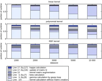
Eight operations were identified where a Matlab implementation of Algorithm 1 spends the bulk of its runtime (varying from 75% to 95% depending on a digit). Seven of these operations pertain to the bottlenecks identified in Section 5.1. Another relatively expensive operation is augmentation of a kernel matrix with a kernel row. Figure 1 shows proportions of runtime spent in the most expensive operations for the digit 8.
0 0.5 1
linear kernel
portion of runtime
0 0.5 1
polynomial kernel
portion of runtime
1000 2000 3000 5000 10 000
0 0.5 1
RBF kernel
portion of runtime
datasize Line 17, Eq.(17) : kappa calculation
Line 17, Eq.(16) : update of matrix Q Line 13 : kernel matrix augmentation Line 3, Eq.(7) : beta calculation
Line 3, Eq.(9) : matrix−vector multiplication Line 3, Eq.(9) : matrix creation from kernel matrix Line 1/3 : kernel calculation
Line 1/3 : matrix creation from input space
Figure 1: Profiling results for digit 8 (MNIST).
The analysis clearly shows that memory access operations dominate the runtime shown in Fig-ure 1. It also reveals that the portion of kernel computation scales down with increasing data size for all three kernels.
5.3 Organization of Matrix Storage and Arithmetic Computations
Having found the weak spots in the Matlab implementation of the incremental SVM, we will now consider the possibilities for the efficiency improvement. In to order gain control over the storage design we choose C++ as an implementation platform. Numerical operations can be efficiently implemented by using the ATLAS library.
5.3.1 STORAGE DESIGN
As it was mentioned before, the difficulty of selection operations in Matlab result from storing ma-trices as one-dimensional arrays. For this type of storage, selection of rows and columns necessarily required a large amount of copying.
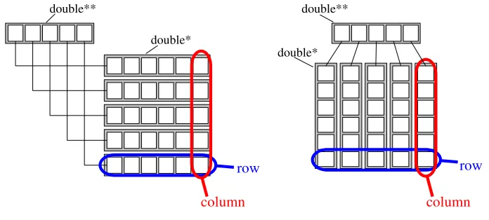
Figure 2: C++ matrix design
An alternative representation of a matrix in C++ is a pointer-to-pointer scheme shown in Fig-ure 2. Depending on whether rows or columns of a matrix are stored in one-dimensional pointed to
double**pointers, either a row-major or a column-major storage is realized.
What are the benefits of a pointer-to-pointer storage for our purposes? Such matrix represen-tation has the advantage that selection along the pointer-of-pointer array requires hardly any time since only addresses of rows or columns need to be fetched. As a result one can completely elimi-nate selection operations in line 1 by storing the input data in a column-major matrix. Furthermore, by storing a kernel matrix in a row-major format (a) additions of kernel rows can be carried out with-out memory relocation, and (b) selections in the matrix Krs are somewhat optimized since r≫s.
Another possible problem arises during addition of a new example when columns have to added to a kernel matrix. This problem can be solved by pre-allocation of columns which can be done in constant-time (amortized).
5.3.2 MATRIXOPERATIONS
Algorithm 3 C++ calculation ofγfor (9) using gaxpy-type matrix-vector multiplication Create an empty vector z
for i=1 :|s|do
z=βi+1Ksi,:+z {gaxpy call}
end for
Computeγ=β1yr+zr+Kcr
Algorithm 4 C++ calculation ofγfor (9) using a naive matrix-vector multiplication Create a matrix Z
Z=yTr; Ksr
Computeγ=βTZ+K
cr {dgemm call}
the problem becomes acute when s grows with the arrival of more and more examples. Yet it turns out to be possible to eliminate even this selection by re-organizing the computation ofγ.
Consider the following form of computing Eq. (9):10
γT =β
1yTr +βT2:endKsr+Kcr. (30)
The first and the last terms are merely vectors, while the middle term is computed using a matrix-vector multiplication and selection over a matrix. Using the transposed matrix Ksr (still stored in a
row-major form) at first seems counter-intuitive, as we argued in the previous section that expensive selection should be carried out over short indices in S and not the long indices in R. However, consider the following observation:
Since s≪r we can just as well run the productβT2:endKs,1:endat a tolerable extra cost of O(ss)arithmetic operations.
By doing so we do not need to worry about selection! The extra s elements in a product vector can be discarded (of course by a selection, however selection over a vector is cheap).
Still another problem with the form (30) of theγ-update remains. If we run it as an inner-product update, i.e. multiplying a row vector with columns of a matrix stored in a row-major format, this loop must be run over the elements in non-contiguous memory. This is as slow as using selection. However, by running it as a gaxpy-type update (e.g. Golub and van Loan, 1996) we end up with loops running over the rows of a kernel matrix, which brings a full benefit of performance-tuned
numerics. The summary of the gaxpy-type computation of γis given in Algorithm 3. For
com-parison, Algorithm 4 shows a naive implementation of theγ-update using inner-product operations (dgemm-type update).
This same construction can be also applied to the inverse matrix update in Eq. (16) by using the following format:
Qi=
βi
κβ+Qi,:. (31)
By doing so explicit creation of a rank-one matrix can be avoided.
To summarize our design, by using the row-major storage of (transposed) matrix K and the gaxpy-type matrix-vector multiplication selection can be avoided by at a cost of extra O(ss) arith-metic operations and performing a selection on a resulting vector.
0 0.5 1
linear kernel
portion of runtime
0 0.5 1
polynomial kernel
portion of runtime
1000 2000 3000 5000 10 000
0 0.5 1
RBF kernel
portion of runtime
datasize
Line 17, Eq.(17) : kappa calculation Line 17, Eq.(16) : update of matrix Q Line 13 : kernel matrix augmentation Line 3, Eq.(7) : beta calculation
Line 3, Eq.(9) : gamma calculation by gaxpy loop Line 1/3 : kernel calculation without matrix creation
Figure 3: C++ runtime proportion digit 8 (MNIST)
5.4 Experimental Evaluation of the New Design
The main goal of the experiments to be presented in this section is to evaluate the impact of the new design of storage and arithmetic operations on the overall performance of incremental SVM learning. In particular, the following issues are to be investigated:
• How is the runtime profile of the main operations affected by the new design?
• How does the overall runtime of the new design scale with an increasing size of a training set?
• What is the overall runtime improvement over the previous implementations and how does it depend on the size of a training set?
To investigate the runtime profiles of the new design, check-pointing has been realized in our C++ implementation. The profiling experiment presented in Section 5.2 (cf. Figure 1) has been repeated for the new design, and the results are shown in Figure 3. The following effects of the new design can be observed:
2. Matrix creation has been likewise eliminated in the computation of γin Line 3. However, the relative cost of the gaxpy computation in the new design remains as high as the relative cost of the combined matrix creation / matrix-vector multiplication operations in the Matlab implementation. The relative cost of theβcomputation is not affected by the new design.
3. Matrix augmentation in Line 13 takes place at virtually no computational cost – due to row-major storage of the kernel matrix.
4. The relative cost of operations in Line 17 is not affected by the new design.
The overall cost distribution of main operations remains largely the same in the new design, kernel computation having the largest weight for small training sets and gamma computation – for the large training sets. However, as we will see from the following experiments, the new design results in major improvement of the absolute running time.
Evaluation of the absolute running time is carried out by means of the scaling factor experiments. The same data set and the same SVM parameters are used as in the profiling experiments. Four implementations of incremental SVM are compared: the original Matlab implementation of C&P (with leave-one-out error estimation turned off), the Matlab implementation of Algorithm 1, the C++ implementation of Algorithms 1 & 3 and the C++ implementation of Algorithms 1 & 4. The latter configuration is used in order to verify that the performance gains indeed stem from the gaxpy-type updates rather than from switching from Matlab to C++.
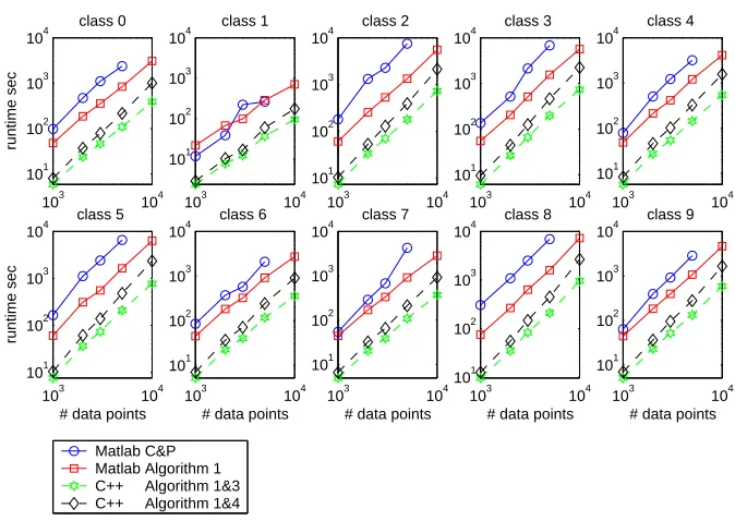
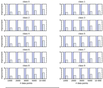
The algorithms are run on the data sets ranging from 1000 to 10000 examples in size, and the training times are plotted against the training set size at a log-log scale. These plots are shown in Figure 4 (for the linear kernel) and 5 (for the RBF kernel). The results for the polynomial kernel are similar to the linear kernel and are not shown. Ten plots are shown separately for each of the digits.
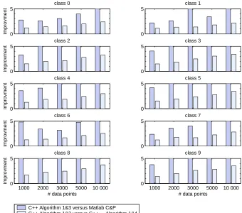
One can see that the C++ implementation significantly outperforms both Matlab implementa-tions. The RBF kernel is more difficult for training than the linear kernel for the MNIST data set, which is reflected by a larger proportion of support vectors (on average 15% for the RBF kernel compared to 5% with the linear kernel, at 10000 training examples). Because of this the experi-ments with the C&P algorithm at 10000 training points were aborted. The Matlab implementation of Algorithm 1 was able to crank about 15000 examples with the RBF kernel, whereas the C++ implementation succeeded to learn 28000 examples, before running out of memory for storing the kernel matrix and the auxiliary data structures (at about 3GB). The relative performance gain of the C++ implementation using gaxpy-updates against the “best Matlab competitor” and against the dgemm-updates is shown in Figure 6 (linear kernel, C&P algorithm) and Figure 7 (RBF kernel, Algorithm 1). Major performance improvement in comparison to Matlab and the naive C++ imple-mentations can be observed, especially visible on larger training set sizes.
6. Applications
103 104 101 102 103 104 class 0 runtime sec
103 104 101
102 103 104
class 1
103 104 101
102 103 104
class 2
103 104 101
102 103 104
class 3
103 104 101
102 103 104
class 4
103 104 101
102 103 104
class 5
# data points
runtime sec
103 104 101
102 103 104
class 6
# data points
103 104 101
102 103 104
class 7
# data points
103 104 101
102 103 104
class 8
# data points
103 104 101
102 103 104
class 9
# data points Matlab C&P
Matlab Algorithm 1 C++ Algorithm 1&3 C++ Algorithm 1&4
Figure 4: Scaling factor plots of incremental SVM algorithms with the linear kernel.
103 104
101 102 103 104 class 0 runtime sec
103 104
101 102 103 104
class 1
103 104
101 102 103 104
class 2
103 104
101 102 103 104
class 3
103 104
101 102 103 104
class 4
103 104
101 102 103 104
class 5
# data points
runtime sec
103 104
101 102 103 104
class 6
# data points
103 104
101 102 103 104
class 7
# data points
103 104
101 102 103 104
class 8
# data points
103 104
101 102 103 104
class 9
# data points
Matlab C&P Matlab Algorithm 1 C++ Algorithm 1&3 C++ Algorithm 1&4
0 5
improvment
class 0
0 5
class 1
0 5
improvment
class 2
0 5
class 3
0 5
improvment
class 4
0 5
class 5
0 5
improvment
class 6
0 5
class 7
1000 2000 3000 5000 10 000 0
5
# data points
improvment
class 8
1000 2000 3000 5000 10 000 0
5
# data points class 9
C++ Algorithm 1&3 versus Matlab C&P C++ Algorithm 1&3 versus C++ Algorithm 1&4
Figure 6: Runtime improvement, linear kernel.
6.1 Learning with Limited Resources
To make SVM learning applicable to very large data sets, a classifier has to be constrained to have a limited number of objects in memory. This is, in principle, exactly what an online classifier with fixed window size M does. Upon arrival of a new example, a least relevant example needs to be removed before a new example can be incorporated. A reasonable criterion for relevance is the value of the weight.
USPS experiment: learning with limited resources. As a proof of concept for learning with limited resources we train an SVM on the USPS data set under the limitations on the number of points that can be seen at a time. The USPS data set contains 7291 training and 2007 images of handwritten digits, size 16×16 (Vapnik, 1998). On this 10-class data set 10 support vector classifiers with a RBF kernel,σ2=0.3·256 and C=100, were trained.11 During the evaluation of a new object, it is assigned to the class corresponding to the classifier with the largest output. The total classification error on the test set for different window sizes M is shown in Figure 8.
One can see that the classification accuracy deteriorates marginally (by about 10%) until the working size of 150, which is about 2% of the data. True, by discarding “irrelevant” examples, one removes potential support vectors that cannot be recovered at a later stage. Therefore one can
0 5
improvment
class 0
0 5
class 1
0 5
improvment
class 2
0 5
class 3
0 5
improvment
class 4
0 5
class 5
0 5
improvment
class 6
0 5
class 7
1000 2000 3000 5000 10 000 0
5
# data points
improvment
class 8
1000 2000 3000 5000 10 000 0
5
# data points class 9
C++ Algorithm 1&3 versus Matlab Algorithm 1 C++ Algorithm 1&3 versus C++ Algorithm 1&4
Figure 7: Runtime improvement, RBF kernel.
50 100 150 200 250 300 350 400 450 500 0
5 10 15 20 25 30
window size
classification error
Figure 8: Test classification errors on the USPS data set, using a support vector classifier (RBF kernel,σ2=0.3·256) with a limited ”window” of training examples.
per each unrestricted 2-class classifier in this experiment is 274. Therefore the results above can be interpreted as reducing the storage requirement by 46% from the minimal at the cost of 10% increase of classification problem.
Notice that the proposed strategy differs from the caching strategy, typical for many SVMlight -like algorithms (Joachims, 1999; Laskov, 2002; Collobert and Bengio, 2001), in which kernel prod-ucts are re-computed if the examples are found missing in the fixed-size cache and the accuracy of the classifier is not sacrificed. Our approach constitutes a trade-off between accuracy and computa-tional load because kernel products never need to be re-computed. It should be noted, however, that computational cost of re-computing the kernels can be very significant, especially for the problems with complicated kernels such as string matching or convolution kernels.
6.2 Active Learning
Another promising application of incremental SVM is active learning. In this scenario, instead of having all data labelled beforehand, an algorithm “actively” chooses examples for which labels must be assigned by a user. Active learning can be extremely successful, if not indispensable, when labelling is expensive, e.g. in computer security or in drug discovery applications.
A very powerful active learning algorithm using SVM was proposed by Warmuth et al. (2003). Assume that the goal of learning is to identify “positive” examples in a data set. The meaning of positivity can vary across applications; for example, it can be binding properties of molecules in drug discovery applications, or hacker attacks in security applications. Selection of a next point to be labelled is carried out in the algorithm of Warmuth et al. (2003) using two heuristics that can be derived from an SVM classifier trained on points with known labels. The “largest positive” heuristic selects the point that has the largest classification score among all examples still unlabeled. The “near boundary” heuristic selects the point whose classification score has the smallest absolute value. Although the semantics of these two heuristics differ – in one case we trying to explore the space of positive examples as fast as possible, whereas in the other case the effort is focused on learning the boundary – in both cases the SVM has to be re-trained after each selection. In the original application of Warmuth et al. (2003) the data samples were relatively small, therefore one could afford re-training SVM from scratch after addition of new points. Obviously, a better way to proceed is by applying incremental learning as presented in this paper.
In the remaining part of this section experiments will be presented that prove the usefulness of active learning in the intrusion detection context. Since the observed data can contain thousands and even millions of examples it is clear that the problem can be addressed only using incremental learning. As a by-product of our experiments, it will be seen that active learning helps to uncover the structure of a learning problem revealed by the number of support vectors.
The underlying data for the experiments is taken from the KDD Cup 1999 data set.12 As a
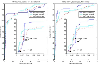
training set, 1000 examples are randomly drawn with an attack rate of 10 percent. The incremental SVM was run with the linear kernel and the RBF kernel withσ=30. An independent set of the same length with the same attack distribution is used for testing. The results are not averaged over multiple repetitions in order not to “disturb” the semantics of different phases of active learning as can be seen from the ROC curves. However, similar behavior was observed over multiple experiments.
KDD Cup experiment: active learning. Consider the following learning scenario. Assume that we can run an anomaly detection tool over our data set which ranks all the points according to
0 0.2 0.4 0.6 0.8 1 0 0.1 0.2 0.3 0.4 0.5 0.6 0.7 0.8 0.9 1
ROC curves, training set, linear kernel
false positive rate
true positive rate
near boundary largest positive anomaly score
0 0.02 0.04 0.06 0.08 0.1 0 0.1 0.2 0.3 0.4 0.5 0.6 0.7 0.8 0.9
i = 60
i = 10
0 0.2 0.4 0.6 0.8 1
0 0.1 0.2 0.3 0.4 0.5 0.6 0.7 0.8 0.9 1
ROC curves, training set, RBF kernel
false positive rate
true positive rate
near boundary largest positive anomaly score
0 0.02 0.04 0.06 0.08 0.1 0 0.1 0.2 0.3 0.4 0.5 0.6 0.7 0.8 0.9
i = 60
i = 10
Figure 9: linear kernel, n=10 and m=50
their degree of anomaly. No labels are needed for this; however, if we know them, we can evaluate anomaly detection by a ROC curve. It is now the goal to use active learning to see if a ROC curve of anomaly detection can be improved.
We take the first n examples with the highest anomaly scores and train a (batch) SVM to obtain an initial model. After that we turn to active learning and learn the next m examples. We are now ready to classify the remaining examples by the trained SVM. The question arises: after spending manual effort to label n+m examples, can we classify the remaining examples better than anomaly
detection?
In order to address this question, an accuracy measure must be defined for our learning scenario. This can be done using the fact that only the ranking of examples according to their scores – and not the score values themselves – matters for the computation of a ROC curve (Cortes and Mohri, 2004). The ranking in our experiment can be defined as follows: the first n examples are ranked according to their anomaly scores, the next m examples are ranked according to their order of inclusion during the active learning phase, and the remaining examples are ranked according to their classification scores.
0 0.2 0.4 0.6 0.8 1 0
0.1 0.2 0.3 0.4 0.5 0.6 0.7 0.8 0.9 1
ROC curves, test set, linear kernel
false positive rate
true positive rate
SVM all SVM reduced near boundary largest positive anomaly score
0 0.2 0.4 0.6 0.8 1
0 0.1 0.2 0.3 0.4 0.5 0.6 0.7 0.8 0.9 1
ROC curves, test set, RBF kernel
false positive rate
true positive rate
SVM all SVM reduced near boundary largest positive anomaly score
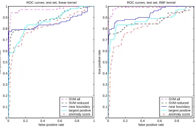
Figure 10: linear kernel, n=10 and m=50
of the two heuristics in the active learning phase was also observed by Warmuth et al. (2003). Yet the “near boundary” heuristic is obviously more suitable for classification, since it explores the boundary region and not merely the region of positive examples.
Another interesting insight can be gained by investigating the behavior of active learning on test data. In this case, supervised learning can also be drawn into comparison. In particular, we consider a full SVM (using a training set size of 1000 examples as opposed to only 60 examples used in the active learning) and a reduced SVM. The latter is obtained from a full SVM by finding a hyperplane closest to a full SVM hyperplane subject to 1-norm regularization over expansion coefficients (cf. Sch¨olkopf et al. (1999)). The regularization constant is chosen such that a reduced SVM has approximately the same number of support vectors as the solution obtain by active learning (in our case the valueλ=2.5 resulted in about 30 support vectors). Thus one can compare active learning with supervised learning given equal complexity of solutions.
7. Discussion and Conclusions
Online learning algorithms have proved to be essential when dealing with (a) very large (see e.g. Le-Cun et al. (1998); Bordes et al. (2005); Tsang et al. (2005)) or (b) non-stationary data (see e.g. Rob-bins and Munro (1951); Murata (1992); Murata et al. (1997, 2002)). While classical neural net-works (e.g. LeCun et al. (1998); Saad (1998)) have a well established online learning toolbox for optimization, incremental learning techniques for Support Vector Machines have been only recently developed (Cauwenberghs and Poggio, 2001; Tax and Laskov, 2003; Martin, 2002; Ma et al., 2003; Ma and Perkins, 2003).
The current paper contributes two-fold to the field of incremental SVM learning. The conver-gence analysis of the algorithm has been performed showing that immediate cycling of the algorithm is impossible provided a kernel matrix is positive semi-definite. Furthermore, we propose a better scheme for organization of memory and arithmetic operations in exact incremental SVM using the gaxpy-type updates of the sensitivity vector. As it is demonstrated by our experiments, the new design results in major constant improvement in the running time of the algorithm.
The achieved performance gains open wide possibilities for application of incremental SVM to various practical problems. We have presented exemplary applications to two possible scenar-ios: learning with limited resources and active learning. Potential applications of incremental SVM learning include, among others, drug discovery, intrusion detection, network surveillance, monitor-ing of non-stationary time series etc. Our implementation is available free of charge for academic use at http://www.mind-ids.org/Software.
It is interesting to compare exact incremental learning to recently proposed alternative ap-proaches to online learning. The recent work of Bordes et al. (2005) presents an online algorithm for L1 SVM, in which a very close approximation of the exact solution is built online before the last gap is bridged in the REPROCESS phase in an offline fashion. This algorithm has been shown to scale well to several hundred thousand examples, however its online solution is not as accurate as the exact solution. It has been observed (cf. Fig. 9 in Bordes et al. (2005)) that the REPROCESS phase may result in major improvement of the test error and may come at a high price in comparison with the online phase, depending on a data set. Another recent algorithm, the Core Vector Machine of Tsang et al. (2005), is based on the L2 formulation of an SVM and has be shown to scale to several million of examples. The idea of this algorithm is to approximate a solution to an L2 SVM by a solution to the two-class Maximal Enclosing Ball problem, for which several efficient online algorithms are known. While scalability results of CVM are very impressive, the approximation of the exact solution can likewise in higher test errors.
The major limilation of the exact incremental learning is its memory requirement, since the set of support vectors must be retained in memory during the entire learning. Due to this limitation, the algorithm is unlikely to be scalable beyond tens of thousands examples; however, for data sizes within this limit it offers an advantage of immediate availablility of the exact solution (crucial in e.g learning of non-stationary problems) and reversibility.
Acknowledgments
The authors are grateful to David Tax and Christian Zillober for fruitful discussions on various top-ics of mathematical optimization that contributed to the development of main ideas of this paper. Ren´e Gerstenberger provided valuable help in the profiling experiments. This work was partially supported by Bundesministerium f¨ur Bildung und Forschung under the project MIND (FKZ 01-SC40A), by Deutsche Forschungsgemeinschaft under the project MU 987/2-1, and by the IST Pro-gramme of the European Community under the PASCAL Network of Excellence, IST-2002-506778. This publication only reflects the authors’ views.
References
D. Angluin. Queries and concept learning. Machine Learning, 2:319–342, 1988.
C. M. Bishop. Neural Networks for Pattern Recognition. Oxford University Press, 1995.
B.. Blankertz, G. Dornhege, C. Sch¨afer, R. Krepki, J. Kohlmorgen, K.-R. M¨uller, V. Kunzmann, F. Losch, and G. Curio. BCI bit rates and error detection for fast-pace motor commands based on single-trial EEG analysis. IEEE Transactions on Neural Systems and Rehabilitation Engineering, 11:127–131, 2003.
A. Bordes, S. Ertekin, J. Wesdon, and L. Bottou. Fast kernel classifiers for online and active learn-ing. Journal of Machine Learning Research, 6:1579–1619, 2005.
G. Cauwenberghs and T. Poggio. Incremental and decremental support vector machine learning. In T. K. Leen, T. G. Dietterich, and V. Tresp, editors, Advances in Neural Information Processing
Systems, volume 13, pages 409–415. MIT Press, 2001.
S. Chakrabarti. Mining the Web: Discovering Knowledge from Hypertext Data. Morgan-Kaufmann, 2002. ISBN 1-55860-754-4.
C.-C. Chang and C.-J. Lin. Libsvm: Introduction and benchmarks. Technical report, Department of Computer Science and Information Engineering, National Taiwan University, Taipei, 2000.
R. Collobert and S. Bengio. SVMTorch: Support vector machines for large-scale regression prob-lems. Journal of Machine Learning Research, 1:143–160, 2001.
C. Cortes and M. Mohri. AUC optimization vs. error rate minimization. In Proc. NIPS’2003, 2004.
E. Eskin, A. Arnold, M. Prerau, L. Portnoy, and S. Stolfo. Applications of Data Mining in
Com-puter Security, chapter A geometric framework for unsupervised anomaly detection: detecting
intrusions in unlabeled data. Kluwer, 2002.
G. H. Golub and C. F. van Loan. Matrix Computations. John Hopkins University Press, Baltimore, London, 3rd edition, 1996.
J. Kivinen, A. J. Smola, and R. C. Williamson. Online learning with kernels. In T. G. Diettrich, S. Becker, and Z. Ghahramani, editors, Advances in Neural Inf. Proc. Systems (NIPS 01), pages 785–792, 2001.
F. Klee and G. J. Minty. How good is the simplex algorithm? In O. Sisha, editor, Inequalities III, pages 159–175. Academic Press, 1972.
P. Laskov. Feasible direction decomposition algorithms for training support vector machines.
Ma-chine Learning, 46:315–349, 2002.
P. Laskov, C. Sch¨afer, and I. Kotenko. Intrusion detection in unlabeled data with quarter-sphere support vector machines. In Proc. DIMVA, pages 71–82, 2004.
Y. LeCun, L. Bottou, G. B. Orr, and K.-R. M¨uller. Efficient backprop. In G. Orr and K.-R. M¨uller, editors, Neural Networks: Tricks of the Trade, volume 1524, pages 9–53, Heidelberg, New York, 1998. Springer LNCS.
N. Littlestone, P. M. Long, and M. K. Warmuth. On-line learning of linear functions. Technical Report CRL-91-29, University of California at Santa Cruz, October 1991.
J. Ma and S. Perkins. Time-series novelty detection using one-class Support Vector Machines. In
IJCNN, 2003. to appear.
J. Ma, J. Theiler, and S. Perkins. Accurate online support vector regression.
http://nis-www.lanl.gov/˜jt/Papers/aosvr.pdf, 2003.
M. Martin. On-line Support Vector Machines for function approximation. Technical report, Uni-versitat Polit`ecnica de Catalunya, Departament de Llengatges i Sistemes Inform`atics, 2002.
N. Murata. A statistical study on the asymptotic theory of learning. PhD thesis, University of Tokyo (In Japanese), 1992.
N. Murata, M. Kawanabe, A. Ziehe, K.-R. M¨uller, and S.-I. Amari. On-line learning in changing environments with applications in supervised and unsupervised learning. Neural Networks, 15 (4-6):743–760, 2002.
N. Murata, K.-R. M¨uller, A. Ziehe, and S. i. Amari. Adaptive on-line learning in changing environ-ments. In M. C. Mozer, M. I. Jordan, and T. Petsche, editors, Advances in Neural Information
Processing Systems, volume 9, page 599. The MIT Press, 1997.
G. Orr and K.-R. M¨uller, editors. Neural Networks: Tricks of the Trade, volume 1524. Springer LNCS, 1998.
J. Platt. Fast training of support vector machines using sequential minimal optimization. In
B. Sch¨olkopf, C. J. C. Burges, and A. J. Smola, editors, Advances in Kernel Methods —
Sup-port Vector Learning, pages 185–208, Cambridge, MA, 1999. MIT Press.
L. Ralaivola and F. d’Alch´e Buc. Incremental support vector machine learning: A local approach.
H. Robbins and S. Munro. A stochastic approximation method. Ann. Math. Stat., 22:400–407, 1951.
S. R¨uping. Incremental learning with support vector machines. Technical Report TR-18, Universit¨at Dortmund, SFB475, 2002.
D. Saad, editor. On-line learning in neural networks. Cambridge University Press, 1998.
B. Sch¨olkopf, S. Mika, C. J. C. Burges, P. Knirsch, K.-R. M¨uller, G. R¨atsch, and A. J. Smola. Input space vs. feature space in kernel-based methods. IEEE Transactions on Neural Networks, 10(5): 1000–1017, September 1999.
B. Sch¨olkopf, J. Platt, J. Shawe-Taylor, A. J. Smola, and R. C. Williamson. Estimating the support of a high-dimensional distribution. Neural Computation, 13(7):1443–1471, 2001.
N. A. Syed, H. Liu, and K. K. Sung. Incremental learning with support vector machines. In SVM
workshop, IJCAI, 1999.
D. Tax and R. Duin. Data domain description by support vectors. In M. Verleysen, editor,
Proc. ESANN, pages 251–256, Brussels, 1999. D. Facto Press.
D. M. J. Tax and P. Laskov. Online SVM learning: from classification to data description and back. In C. et al. Molina, editor, Proc. NNSP, pages 499–508, 2003.
I. Tsang, J. Kwok, and P.-M. Cheung. Core Vector Machines: fast SVM training on very large data sets. Journal of Machine Learning Research, 6:363–392, 2005.
V. N. Vapnik. Statistical Learning Theory. Wiley, New York, 1998.
M. K. Warmuth, J. Liao, G. R¨atsch, M. Mathieson, S. Putta, and C. Lemmem. Support Vector Machines for active learning in the drug discovery process. Journal of Chemical Information