A Generalized Maximum Entropy Approach to Bregman
Co-clustering and Matrix Approximation
Arindam Banerjee [email protected]
Department of Computer Science and Engineering University of Minnesota, Twin Cities
Minneapolis, MN, USA
Inderjit Dhillon [email protected]
Department of Computer Sciences University of Texas at Austin Austin, TX, USA
Joydeep Ghosh [email protected]
Department of Electrical and Computer Engineering University of Texas at Austin
Austin, TX, USA
Srujana Merugu [email protected]
Yahoo! Research Santa Clara, CA, USA
Dharmendra S. Modha [email protected]
IBM Almaden Research Center San Jose, CA, USA
Editor: John Lafferty
Abstract
vari-ety of problem domains and also describe novel co-clustering applications such as missing value prediction and compression of categorical data matrices.
Keywords: co-clustering, matrix approximation, Bregman divergences, Bregman information, maximum entropy
1. Introduction
Data naturally arises in the form of matrices in a multitude of machine learning and data mining applications. Often, the data matrices that arise in real-world applications contain a large number of rows and columns, and may be very sparse. Understanding the natural structure of such matrices is a fundamental problem.
Clustering is an unsupervised learning technique that has been often used to discover the “latent structure” of data matrices that describe a set of objects (rows) by their feature values (columns). Typically, a clustering algorithm strives to group “similar” objects (or rows). A large number of clustering algorithms such as kmeans, agglomerative clustering, and their variants have been thor-oughly studied (Jain and Dubes, 1988; Ghosh, 2003). Often, clustering is preceded by a dimension-ality reduction phase, such as feature selection where only a subset of the columns is retained. As an alternative to feature selection, one can cluster the columns, and then represent each resulting group of features by a single derived feature (Dhillon et al., 2003a).
A recent paper (Dhillon and Modha, 2001) dealing with the spherical kmeans algorithm for clustering large, sparse document-term matrices arising in text mining graphically demonstrates (see Figures 13, 31, and 32 in the paper by Dhillon and Modha, 2001) that document clustering naturally brings together similar words. Intuitively, documents are similar because they use similar words. A natural question is whether it is possible to mathematically capture this relationship between rows and columns. Furthermore, is it possible to exploit this relationship to a practical advantage? This paper shows that both these questions can be answered in the affirmative in the context of clustering. Co-clustering, also called bi-clustering (Hartigan, 1972; Cheng and Church, 2000), is the prob-lem of simultaneously clustering rows and columns of a data matrix. Unlike clustering which seeks similar rows or columns, co-clustering seeks “blocks” (or “co-clusters”) of rows and columns that are inter-related. Co-clustering has recently received a lot of attention in several practical applica-tions such as simultaneous clustering of documents and words in text mining (Dhillon et al., 2003b; Gao et al., 2005; Takamura and Matsumoto, 2003), genes and experimental conditions in bioin-formatics (Cheng and Church, 2000; Cho et al., 2004; Kluger et al., 2003), tokens and contexts in natural language processing (Freitag, 2004; Rohwer and Freitag, 2004; Li and Abe, 1998), users and movies in recommender systems (George and Merugu, 2005), etc.
Co-clustering is desirable over traditional “single-sided” clustering from a number of perspec-tives:
1. Simultaneous grouping of row and column clusters is more informative and digestible. Co-clustering provides compressed representations that are easily interpretable while preserving most of the information contained in the original data, which makes it valuable to a large class of statistical data analysis applications.
param-eters and hence, a much more compact representation for subsequent analysis. Since co-clustering incorporates row co-clustering information into column co-clustering and vice versa, one can think of it as a “statistical regularization” technique that can yield better quality clusters even if one is primarily interested in a single-sided clustering. The statistical regularization effect of co-clustering is extremely important when dealing with large, sparse data matrices, for example, those arising in text mining. A similar intuition can be drawn from subspace clustering methods (Parsons et al., 2004), which only use a part of the full potential of the co-clustering methodology.
3. As the size of data matrices increases, so does the need for scalable clustering algorithms. Single-sided, geometric clustering algorithms such as kmeans and its variants have computa-tion time proporcomputa-tional to mnk per iteracomputa-tion, where m is the number of rows, n is the number of columns and k is the number of row clusters. Co-clustering algorithms based on a similar iterative process, on the other hand, involve optimizing over a smaller number of parameters, and can relax this dependence to O(mkl+nkl)where m,n and k are defined as before and l is the number of column clusters. Since the number of row and column clusters is usually much smaller than the original number of rows and columns, co-clustering can lead to substantial reduction in the running time (see, for example, Dhillon et al. 2003b and Rohwer and Freitag 2004).
In summary, co-clustering is an exciting paradigm for unsupervised data analysis in that it is more informative, has less parameters, is scalable, and is able to effectively intertwine row and column information.
1.1 ITCC: A Motivating Example
Let X and Y be discrete random variables that take values in the sets {xu}, [u]m1,and{yv}, [v]n1, respectively, where [u]m
1 denotes an index u running over {1,· · ·,m}. Information-theoretic co-clustering provides a principled approach for simultaneously co-clustering the rows and columns of the joint probability distribution p(X,Y). In practice, the entries of this matrix may not be known and are, instead, estimated from a contingency table or co-occurrence matrix. Let the row clusters be denoted by{xˆg}, [g]k1 and the column clusters by{yˆh}, [h]l1. Let ˆX and ˆY denote the clustered random variables induced by X and Y that range over the set of row and column clusters respectively. A natural goal is to choose a co-clustering that preserves the maximum amount of “information” in the original data. In particular, since the data corresponds to the joint probability distribution of random variables X and Y , it is natural to preserve the mutual information between X and Y , or, in other words, minimize the loss in mutual information due to the compression that results from co-clustering. Thus, a suitable formulation is to solve the problem:
min ˆ
X,Yˆ
(I(X ;Y)−I(X ; ˆˆ Y)), (1)
where I(X ;Y)is the mutual information between X and Y (Cover and Thomas, 1991). Dhillon et al. (2003b) showed that
I(X ;Y)−I(X,ˆ Yˆ) =KL(p(X,Y)||q(X,Y)), (2) where q(X,Y)is a distribution of the form
q(X,Y) =p(Xˆ,Yˆ)p(X|Xˆ)p(Y|Yˆ), (3)
and KL(·||·)denotes the Kullback-Leibler(KL) divergence, also known as relative entropy. Thus, the search for the optimal co-clustering may be conducted by searching for the nearest approximation q(X,Y) that has the above form. Since p(X), p(Y) and p(Xˆ,Yˆ) are determined by m−1, n−1 and kl−1 parameters respectively, with k+l dependencies due to p(Xˆ)and p(Yˆ), for a given co-clustering the distribution q(X,Y)depends only on(kl+m+n−k−l−3)independent parameters, which is much smaller than the mn−1 parameters that determine a general joint distribution. Hence, q(X,Y)is a “low-complexity” or low-parameter matrix approximation of p(X,Y).
The above viewpoint was developed by Dhillon et al. (2003b). We now present an alternate viewpoint that will enable us to generalize our approach to arbitrary data matrices and general distortion measures. The following lemma highlights a key maximum entropy property that makes q(X,Y)a “low-complexity” or low-parameter approximation.
Lemma 1 Given a fixed co-clustering, consider the set of joint distributions p0 that preserve the row, column and co-cluster marginals of the input distribution p:
∑
x∈xˆ
∑
y∈ˆyp0(x,y) =p(x,ˆ yˆ) =
∑
x∈xˆ
∑
y∈ˆyp(x,y), ∀x,ˆ y,ˆ (4)
p0(x) =p(x), p0(y) =p(y), ∀x,y. (5) Among all such distributions p0, the distribution q given in (3) has the maximum entropy, that is, H(q(X,Y))≥H(p0(X,Y)).
product distribution p(X)p(Y) has maximum entropy (see Cover and Thomas, 1991, Problem 5, Chapter 11). The above lemma states that among all distributions that preserve row, column, and co-cluster marginals, that is, (4) and (5) hold, the maximum entropy distribution has the form in (3). The maximum entropy characterization ensures that q(X,Y)has a number of desirable properties. For instance, given the row, column and co-cluster marginals, it is the unique distribution that satisfies certain consistency criteria (Csisz´ar, 1991; Shore and Johnson, 1980). In Section 4, we also demon-strate that it is the optimal approximation to the original distribution p in terms of KL-divergence among all multiplicative combinations of the preserved marginals. It is important to note that the maximum entropy characterization also implies that q is a low-complexity matrix approximation.1 In contrast, note that the input p(X,Y)obviously satisfies the constraints in (4) and (5), but in gen-eral, is determined by(mn−1)parameters and has lower entropy than q. Every co-clustering yields a unique maximum entropy distribution. Thus, by (2) and Lemma 1, the co-clustering problem (1) is equivalent to the problem of finding the nearest (in KL-divergence) maximum entropy distribution that preserves the row, column and co-cluster marginals of the original distribution. The maximum entropy property in Lemma 1 may be re-stated as KL(q||p0)≤KL(p0||p0), where p0is the uniform distribution. Thus, the maximum entropy principle is identical to the minimum relative entropy principle where the relative entropy is measured with respect to p0.
The above formulation is applicable when the data matrix corresponds to an empirical joint distribution. However, there are important situations when the data matrix cannot be interpreted in this matter, for example the matrix may contain negative entries and/or a distortion measure other than KL-divergence, such as the squared Euclidean distance might be more appropriate.
1.2 Key Contributions
The contributions of this paper can be summarized as follows:
• We introduce a partitional co-clustering formulation driven by a matrix approximation view-point where the quality of clustering is characterized by the accuracy of an induced co-clustering-based matrix approximation, measured in terms of a suitable distortion measure. This formulation serves the dual purpose of (i) obtaining row and column clusterings that optimize a well-defined global objective function, and (ii) providing a new class of desirable matrix approximations.
• Our formulation is applicable to all Bregman divergences (Azoury and Warmuth, 2001; Baner-jee et al., 2005b; Bregman, 1967; Censor and Zenios, 1998), which constitute a large class of distortion measures including the most commonly used ones such as squared Euclidean dis-tance, KL-divergence, Itakura-Saito disdis-tance, etc. The generalization to Bregman divergences is useful due to a bijection between regular exponential families and a sub-class of Bregman divergences called regular Bregman divergences (Banerjee et al., 2005b). This bijection re-sult enables us to choose the appropriate Bregman divergence based on the underlying data generation process or noise model. This, in turn, allows us to perform co-clustering on a wide variety of data matrices.
• Our formulation allows multiple co-clustering schemes wherein the reconstruction of the orig-inal matrix is based on different sets of linear summary statistics that one may be interested
in preserving. In particular, we focus on summary statistics that correspond to conditional expectations over partitions that result from the rows, columns and co-clusterings. We es-tablish that there are exactly six non-trivial co-clustering schemes. Each of these schemes corresponds to a unique co-clustering basis, that is, combination of conditional expectations over various partitions. Using a formal abstraction, we explicitly enumerate and analyze the co-clustering problem for all the six bases. Existing partitional co-clustering algorithms (Cho et al., 2004; Dhillon et al., 2003b) can then be seen as special cases of the abstraction, em-ploying one of the six co-clustering bases. Three of the six bases we discuss have not been used in the literature till date.
• Previous work on co-clustering assume that all the elements of the data matrix are equally important, that is, have uniform measure. In contrast, we associate a probability measure with the elements of the specified matrix and pose the co-clustering problem in terms of the random variable that takes values among the matrix elements following this measure. Our formulation based on random variables provides a natural mechanism for handling values with differing levels of uncertainty and in particular, missing values, while retaining both the analytical and algorithmic simplicity of the corresponding uniform-measure formulation.
• En route to formulating the Bregman co-clustering problem, we introduce the minimum Breg-man information (MBI) principle that generalizes the well-known maximum entropy and stan-dard least-squares principles to all Bregman loss functions. The co-clustering process is guided by the search for the matrix approximation that has the minimum Bregman informa-tion while preserving the specified co-clustering statistics.
• We provide an interpretation of the Bregman co-clustering problem in terms of minimizing the loss in Bregman information due to co-clustering, which enables us to generalize the viewpoint presented in information-theoretic co-clustering (Dhillon et al., 2003b).
• We develop an efficient meta co-clustering algorithm based on alternate minimization that is guaranteed to achieve (local) optimality for all Bregman divergences. Many previously known parametric clustering and clustering algorithms such as minimum sum-squared residue co-clustering (Cho et al., 2004) and information-theoretic co-co-clustering (Dhillon et al., 2003b) follow as special cases of our methodology.
• Lastly, we describe some novel applications of co-clustering such as predicting missing values and compression of categorical data matrices, and also provide empirical results comparing different co-clustering schemes for various application domains.
In summary, our results provide a sound theoretical framework for the analysis and design of efficient co-clustering algorithms for data approximation and compression, and considerably expand applicability of the co-clustering methodology.
1.3 Outline of the Paper and Notation
to provide intuition about the main results. Then, in Section 4, we enumerate various possible co-clustering bases corresponding to the summary statistics chosen to be preserved, and present a general formulation that is applicable to all these bases. In Section 5, we analyze the general Bregman co-clustering problem and propose a meta-algorithm that is applicable to all Bregman di-vergences and all co-clustering bases. In Appendix E, we describe how the Bregman co-clustering algorithm can be instantiated for various choices of Bregman divergence and co-clustering basis by providing the exact update steps. Readers interested in a purely computational recipe can jump to Apendix E. Empirical evidence on the benefits of co-clustering and preliminary experiments on novel co-clustering applications are presented in Section 6. We discuss related work in Section 7 and conclude in Section 8.
A brief word about the notation: Sets such as {x1,· · ·,xn} are enumerated as{xi}ni=1 and an
index i running over the set{1,· · ·,n}is denoted by[i]n
1. Random variables are denoted using upper case letters, for example, Z. Matrices are denoted using upper case bold letters, for example, Z, whereas the corresponding lower case letters zuvdenote the matrix elements. Transpose of a matrix
Z is denoted by ZT. The effective domain of a function f is denoted by dom(f)and the inverse of a function f , when well defined, is denoted by f(−1). The relative interior and boundary of a set
S
are denoted by ri(S
)and bd(S
)respectively. Tables 15, 16 and 17 list the notation used in the paper.2. Preliminaries
In this section, we discuss some important properties of Bregman divergences and also describe the basic setup of our co-clustering framework.
2.1 Bregman Divergences and Bregman Information
We start by defining Bregman divergences (Bregman, 1967; Censor and Zenios, 1998), which form a large class of well-behaved loss functions with a number of desirable properties.
Definition 1 Letφbe a real-valued convex function of Legendre type2(Rockafellar, 1970; Banerjee et al., 2005b) defined on the convex set
S
≡dom(φ) (⊆Rd). The Bregman divergence dφ:
S
×ri(
S
)7→R+ is defined asdφ(z1,z2) =φ(z1)−φ(z2)− hz1−z2,∇φ(z2)i,
where∇φis the gradient ofφ.
Example 1.A (I-Divergence) Given z∈R+, let φ(z) =z log z−z . For z1,z2∈R+, dφ(z1,z2) = z1log(z1/z2)−(z1−z2).
Example 2.A (Squared Euclidean Distance) Given z∈R, letφ(z) =z2. For z1,z2∈R, dφ(z1,z2) = (z1−z2)2.
Example 3.A (Itakura-Saito Distance) Given z∈R+, letφ(z) =−log z . For z1,z2∈R+, dφ(z1,z2) =
z1 z2 −log
z1 z2
−1 .
2. A proper, closed convex functionφis said to be of Legendre type if (i) int(dom(φ))is non-empty, (ii)φis strictly convex and differentiable on int(dom(φ)), and (iii)∀zb∈bd(dom(φ)), lim
z→zb
Given a Bregman divergence and a random variable, the uncertainty in the random variable can be captured in terms of a useful concept called Bregman information (Banerjee et al., 2005b) defined below.
Definition 2 For any Bregman divergence dφ :
S
×int(S
) 7→R+ and any random variable Z ∼w(z), z∈
Z
⊆S
, the Bregman information of Z is defined as the expected Bregman divergence to the expectation, that is,Iφ(Z) =E[dφ(Z,E[Z])].
Intuitively, this quantity is a measure of the “spread” or the “information” in the random variable.
Example 1.B (I-Divergence) Given a random variable Z∼w(z),z∈
Z
⊆R+, the Bregman infor-mation corresponding to I-divergence is given byIφ(Z) =E[Z log(Z/E[Z])−Z+E[Z]] =E[Z log(Z/E[Z])].
When w is the uniform measure and the support of Z (say
Z
) consists of joint probability values of two other random variables X and Y , that is,Z
={p(xu,yv), [u]m1,[v]n1}, then E[Z] = mn1 , that is,probability value corresponding to the uniform distribution p0(X,Y). The Bregman information in this case is given by
Iφ(Z) = 1 mn
m
∑
u=1
n
∑
v=1
p(xu,yv)log
p(xu,yv)
p0(xu,yv)
= 1
mnKL(p||p0) =− 1
mnH(p) +constant,
where H(·)is the Shannon entropy.
Example 2.B (Squared Euclidean Distance) Given Z∼w(z), z∈
Z
⊆R, the Bregman informa-tion corresponding to squared Euclidean distance is given byIφ(Z) =E[Z−E[Z]]2,
which is the variance of Z. When w is uniform and the support of Z, that is,
Z
consists of elements in a matrix Z∈Rm×n, that is,Z
={zuv,[u]m1,[v]n1}, then E[Z] =mn1 ∑u=m 1∑nv=1zuv≡¯z. The Bregmaninformation in this case is given by
Iφ(Z) = 1 mn
m
∑
u=1
n
∑
v=1
(zuv−¯z)2=
1 mn
m
∑
u=1
n
∑
v=1
z2uv−¯z2= 1 mnkZk
2
F+constant,
that is, a linear function of the squared Frobenius norm of Z.
We note a useful property of Bregman information that will be extensively used in subsequent sections. The property, formally stated below, shows that the Bregman information exactly equals the difference between the two sides of Jensen’s inequality (Cover and Thomas, 1991).
Lemma 2 (Banerjee et al., 2005b) For any Bregman divergence dφ :
S
×ri(S
)7→R+ and ran-dom variable Z∼w(z), z∈Z
⊆S
, the Bregman information Iφ(Z) =E[dφ(Z,E[Z])] =E[φ(Z)]−φ(E[Z]).
2.2 Data Matrix
We focus on the problem of co-clustering a specified m×n data matrix Z. Let each entry of Z= [zuv]
take values in the convex set3
S
=dom(φ), for example,S
=R for φ(z) =z2 andS
=R+ forφ(z) =z log z−z. Hence, Z∈
S
m×n. Observe that we are now admitting a much larger class ofmatrices than those used in the co-clustering formulations of Cho et al. (2004) and Dhillon et al. (2003b).
Given the data matrix Z, we consider a random variable Z, that takes values in Z following a probability measure as described below. Let U be a random variable that takes values in{1,· · ·,m}, the set of row indices, and let V be a random variable that takes values in {1,· · ·,n}, the set of column indices. Let(U,V)be distributed according to a probability measure w={wuv:[u]m1,[v]n1}, which is either pre-specified or set to be the uniform distribution.4 Let Z be a(U,V)-measurable random variable that takes values in Z following w, that is, p(Z(u,v) =zuv) =wuv. Clearly, for a
given matrix Z, the random variable Z is a deterministic function of the random variable (U,V). Throughout the paper, we assume the matrix Z and the measure w to be fixed so that taking con-ditional expectations of the random variable Z is well defined. In pure numeric terms, such condi-tional expectations are simply weighted row/column/block averages of the matrix Z according to the weights w. The stochastic formalization enables a succinct way to analyze such weighted averages.
Example 1.C (I-Divergence) Let(X,Y)∼p(X,Y)be jointly distributed random variables with X and Y taking values in{xu},[u]m1 and{yv},[v]n1 respectively. Then, p(X,Y) can be written in the
form of the matrix Z= [zuv],[u]m1,[v]n1, where zuv=p(xu,yv)is a deterministic function of u and v.
This example with a uniform measure w corresponds to the setting described in Section 2, Example 1.B (originally in the work of Dhillon et al., 2003b).
Example 2.C (Squared Euclidean Distance) Let Z∈Rm×ndenote a data matrix whose elements
may assume positive, negative, or zero values and let w be a uniform measure. This example corresponds to the co-clustering setting described by Cheng and Church (2000) and Cho et al. (2004).
2.3 Bregman Co-clustering
We define a k×l partitional co-clustering as a pair of functions:
ρ:{1,· · ·,m} 7→ {1,· · ·,k},
γ:{1,· · ·,n} 7→ {1,· · ·,l}.
Let ˆU and ˆV be random variables that take values in{1,· · ·,k}and{1,· · ·,l}such that ˆU=ρ(U)and ˆ
V =γ(V). Let ˆZ= [ˆzuv]∈
S
m×nbe an approximation for the data matrix Z such that ˆZ depends onlyupon a given co-clustering(ρ,γ)and certain summary statistics derived from the co-clustering. Let ˆ
Z be a(U,V)-measurable random variable that takes values in this approximate matrix ˆZ following
3.Sneed not necessarily be a subset ofR. It is convenient to assume this for ease of exposition. In general, the elements of the matrix Z can take values over any convex domain with a well-defined Bregman divergence. We give examples of such settings in Section 6.
w, that is, p(Zˆ(U,V) = ˆzuv) =wuv. Then the goodness of the underlying co-clustering can be measured in terms of the expected distortion between Z and ˆZ, that is,
E[dφ(Z,Zˆ)] =
m
∑
u=1
n
∑
v=1
wuvdφ(zuv,ˆzuv) =dΦw(Z,Z)ˆ , (6)
whereΦw:
S
m×n7→Ris a separable convex function induced on the matrices such that the Breg-man divergence between any pair of matrices is the weighted sum of the element-wise BregBreg-man divergences corresponding to the convex functionφ. From the matrix approximation viewpoint, the above quantity is simply the weighted element-wise distortion between the given matrix Z and the approximation ˆZ. The co-clustering problem is then to find(ρ,γ) such that (6) is minimized. To carry out this plan, we need to make precise the connection between(ρ,γ)and ˆZ.Example 1.D (I-Divergence) The Bregman co-clustering objective function (6) in this case is given by E[dφ(Z,Zˆ)] =E[Z log(Z/Zˆ)−Z+Zˆ].
Example 2.D (Squared Euclidean Distance) The Bregman co-clustering objective function (6) in this case is given by E[dφ(Z,Zˆ)] =E[(Z−Zˆ)2].
The goodness of a co-clustering (ρ,γ)is determined by how well ˆZ (or the matrix ˆZ) approx-imates Z (or the matrix Z). The crucial thing to note is that the construction of the approximation
ˆ
Z is based on the co-clustering (ρ,γ) and certain summary statistics of the original random vari-able Z that one wants to preserve in the approximation. The summary statistics may be properties of the co-clusters themselves, such as co-cluster marginals as in (4), and/or some other important statistics of the data, such as row and column marginals as in (5). Note that Z is not accessible while constructing ˆZ, since otherwise one could just set ˆZ=Z and get perfect reconstruction. The special case when ˆZ is constructed only using the co-clustering(ρ,γ)and the co-cluster marginals is important and easy to understand. Moreover, it is a straightforward generalization of one-sided clustering schemes such as kmeans. Hence, we first investigate this special case in detail in the next section. The general case, where additional summary information such as row/column marginals of the original matrix are available, will be analyzed in Sections 4 and 5.
3. Block Average Co-clustering: A Special Case
In this section, we discuss the important special case of Bregman co-clustering where the summary statistics are derived by aggregating along the co-clusters, that is, the summary statistics preserved are just the co-cluster means. Hence, in this case, for a given co-clustering(ρ,γ), ˆZ has to be re-constructed based only on the co-cluster means, or equivalently, the conditional expectation random variable E[Z|U,ˆ Vˆ]where expectation is taken with respect to the measure w.5 The quality of the co-clustering(ρ,γ)is determined by the approximation error between Z and ˆZ.
3.1 Minimum Bregman Information (MBI) Principle
In order to analyze the block co-clustering problem, we first focus on characterizing the approx-imation random variable ˆZ given a fixed co-clustering (ρ,γ) and the resulting co-cluster means
{E[Z|u,ˆ vˆ]}. While there can be many different ways to get an approximation ˆZ from the available information, we consider a principled characterization based on the Bregman information of the reconstruction ˆZ. In particular, we propose and use the minimum Bregman information principle that can be shown to be a direct generalization of the maximum entropy as well as the least squares principles.
In order to get the “best” approximation, we consider a special class of approximating random variables Z0 based on the given co-clustering and the available information E[Z|U,ˆ Vˆ]. Let
S
A bedefined as
S
A={Z0|E[Z0|u,ˆ vˆ] =E[Z|u,ˆ vˆ], ∀[uˆ]1k,[vˆ]l1}. (7) It is reasonable to search for the best approximation inS
A since any random variable Z0 in thisclass has the same co-cluster statistics as the original random variable Z. In other words, the cor-responding reconstructed matrices preserve the co-cluster statistics of the original matrix, which is desirable. Then, with respect to the set
S
A, we ask: What is the “best” random variable to select fromthis set? We propose a new minimum Bregman information principle that recommends selecting a random variable that has the minimum Bregman information subject to the linear constraints (7):
ˆ
ZA ≡ ZˆA(ρ,γ) =argmin Z0∈S
A
Iφ(Z0). (8)
The basic philosophy behind the minimum Bregman information principle is that the “best” approximation given certain information is one that does not make any extra assumptions over the available information. Mathematically, the notion of no extra assumptions or maximal uncertainty translates to minimum Bregman information while the available information is provided by the linear constraints that preserve the specified statistics.
As the following examples show, the widely used maximum entropy principle (Jaynes, 1957; Cover and Thomas, 1991) and standard least squares principles (Csisz ´ar, 1991) can be obtained as special cases of the MBI principle.
Example 1.E From Example 1.B, we observe that the Bregman information of a random variable Z following a uniform distribution over the joint probability values of two other random variables X and Y is given by− 1
mnH(p(X,Y))upto an additive constant, that is, it is negatively related to entropy
of the joint distribution of X and Y . Hence, minimizing the Bregman information is equivalent to maximizing the entropy demonstrating that the maximum entropy principle is a special case of the MBI principle corresponding to I-divergence.
Example 2.E From Example 2.B, we observe that the Bregman information of a random variable Z following a uniform distribution over the elements of a matrix Z is given by mn1 kZk2
Fupto an additive
constant. Hence, minimizing the Bregman information in this case is equivalent to minimizing the Frobenius norm of the matrix (L2norm for a vector), which in turn implies that the standard least squares principle is a special case of the MBI principle corresponding to squared error.
Now, we focus on getting a closed form solution of the minimum Bregman information prob-lem. In the absence of any constraints, the minimum Bregman information solution corresponds to a constant random variable. For the current situation, where we are constrained to preserve the co-cluster means{E[Z|u,ˆ vˆ]}, the following theorem shows that the best approximation ˆZA simply
Theorem 1 The solution to (8) is unique and is given by
ˆ
ZA=E[Z|Uˆ,Vˆ].
Proof Let Z0be any random variable in
S
Aand let ˆZAdenote E[Z|Uˆ,Vˆ]. By definition,Iφ(Z0) (a)= E[φ(Z0)]−φ(E[Z0])
= E[φ(Z0)]−EUˆ,Vˆ[φ(E[Z0|Uˆ,Vˆ])] +EUˆ,Vˆ[φ(E[Z0|U,ˆ Vˆ])]−φ(E[Z0])
(b)
= E[φ(Z0)]−EUˆ,Vˆ[φ(E[Z0|Uˆ,Vˆ])] +EUˆ,Vˆ[φ(ZˆA)]−φ(EUˆ,Vˆ[ZˆA]) (c)
= EUˆ,Vˆ
h
EZ0|Uˆ,Vˆ[φ(Z0)]−φ(E[Z0|Uˆ,Vˆ])
i
+Iφ(ZˆA)
(d)
≥ Iφ(ZˆA),
where (a) and (c) follow from Lemma 2; (b) follows from the fact that E[Z0|U,ˆ Vˆ] =E[Z|U,ˆ Vˆ] =ZˆA and EUˆ,Vˆ[E[Z|U,ˆ Vˆ]] =EUˆ,Vˆ[ZˆA] =E[Z] =E[Z0]; and (d) follows from conditional Jensen’s
inequal-ity. In particular, sinceφis convex, we have EZ0|Uˆ,Vˆ[φ(Z0)]≥φ(E[Z0|Uˆ,Vˆ]).
Hence, ˆZA has lower Bregman information than any random variable in
S
A. Further, ˆZA∈S
A,that is, E[ZˆA|U,ˆ Vˆ] =ZˆA=E[Z|U,ˆ Vˆ]. Along with the strict convexity ofφ, this ensures that ˆZA=
E[Z|Uˆ,Vˆ]is the unique solution to (8).
For an alternative constructive proof of Theorem 1, please see Appendix C.
Besides being the MBI solution, ˆZAhas an additional important property that makes it the “best”
reconstruction. Although we focused on the set
S
Athat contains all Z0that preserve the knownco-cluster statistics, an alternative could have been to investigate the set
S
B that contains alldetermin-istic functions of the available information E[Z|Uˆ,Vˆ], that is,
S
B={Z00|Z00=f(E[Z|U,ˆ Vˆ])}, (9)where f is an arbitrary(Uˆ,Vˆ)-measurable function. In
S
B, the optimal approximation ˆZBis the one that is closest to the true Z:ˆ
ZB ≡ argmin Z00∈S
B
E[dφ(Z,Z00)]. (10)
In order to show a relationship between ˆZAand ˆZB, we start with the following lemma (Lemma 3),
which establishes the fact that the MBI solution ˆZA allows a Pythagorean decomposition of the
expected divergence between any Z0∈
S
A and any Z00∈S
B.6 Recall thatS
Aconsists of all randomvariables that have the same co-cluster statistics as Z and
S
Bconsists of all measurable functions ofE[Z|Uˆ,Vˆ].
Lemma 3 For any Z0∈
S
Aas in (7), any Z00∈S
Bas in (9), and ˆZAas in (8),E[dφ(Z0,Z00)] =E[dφ(Z0,ZˆA)] +E[dφ(ZˆA,Z00)].
A proof of the lemma is presented in Appendix C. Now, since ˆZA =E[Z|Uˆ,Vˆ], and is hence a
function of E[Z|U,ˆ Vˆ], we have ˆZA∈
S
B. As a result, from Lemma 3, we get the following projection theorem, which states that the MBI solution ˆZAis the “forward” Bregman projection of any elementof
S
Aonto the setS
Bas well as the “backward” Bregman projection of any element ofS
Bonto theset
S
A.Theorem 2 (Projection Theorem) For any Z0∈
S
A as in (7), any Z00∈S
B as in (9), and ˆZA asin (8), we have,
(a) ˆZA=argmin Z0∈S
A
E[dφ(Z0,Z00)],
(b) ˆZA=argmin Z00∈S
B
E[dφ(Z0,Z00)].
A proof of the theorem is presented in Appendix C. Since the original Z ∈
S
A, we observe thatˆ
ZA is the best approximation (by a backward Bregman projection) to Z in
S
B, implying ˆZB=ZˆAasformally stated below.
Corollary 1 For ˆZAand ˆZBgiven by (8) and (10) respectively, we have
ˆ
Z≡ZˆA=ZˆB. (11)
The equivalence result is a precise mathematical quantification of the optimal approximation prop-erty of the MBI solution for the special case where only E[Z|U,ˆ Vˆ]is available during reconstruction. It shows that the best approximation in terms of expected Bregman divergence given the co-cluster statistics is indeed the MBI solution that preserves those statistics.
3.2 Co-clustering Problem Formulation
Now that we have associated an approximation ˆZ with a given co-clustering (ρ,γ), we return to the original Bregman co-clustering problem in (6). The goal is to obtain a co-clustering (ρ,γ) such that the expected Bregman divergence between Z and the approximation ˆZ is minimized. So far, we know that the best reconstruction ˆZ is the MBI solution and is expressed in closed form by Theorem 1. The following lemma presents an alternative characterization of the co-clustering objective function (6). It shows that the expected Bregman divergence to the approximation ˆZ is exactly equal to the loss in Bregman information due to co-clustering.
Lemma 4 For any random variable Z and ˆZ as in (11),
Proof By definition,
E[dφ(Z,Zˆ)] = E[φ(Z)−φ(Zˆ)− hZ−Z,ˆ ∇φ(Zˆ)i]
(a)
= E[φ(Z)]−E[φ(Zˆ)]−Eˆ
U,Vˆ[hE[Z|U,ˆ Vˆ]−E[Zˆ|U,ˆ Vˆ],∇φ(Zˆ)i]
(b)
= E[φ(Z)]−E[φ(Zˆ)]
(c)
= E[φ(Z)]−φ(E[Z])−E[φ(Zˆ)] +φ(E[Zˆ])
(d)
= Iφ(Z)−Iφ(Zˆ),
where (a) follows from the fact that ˆZ and hence, ∇φ(Zˆ)is constant for fixed(U,ˆ Vˆ), (b) follows since ˆZ∈
S
A, (c) follows since E[Z] =E[Zˆ]and (d) follows from Lemma 2.Using Lemma 4, the original Bregman clustering problem in (6) can be posed as one of finding the optimal co-clustering(ρ∗,γ∗)defined as follows:
(ρ∗,γ∗) = argmin
(ρ,γ)
E[dφ(Z,Zˆ)] = argmin
(ρ,γ)
[Iφ(Z)−Iφ(Zˆ)] = argmax
(ρ,γ)
Iφ(Zˆ), (12)
since Iφ(Z)is a constant. Further, using the fact that ˆZ is the solution to the MBI problem, we have
(ρ∗,γ∗) = argmax
(ρ,γ)
min
Z0∈S
A
Iφ(Z0). (13)
Hence, the best co-clustering(ρ∗,γ∗)is the one that results in the matrix reconstruction correspond-ing to the minimum approximation error, or equivalently, the one that solves the max-min problem in (13).
3.3 Block Average Co-clustering Algorithm
In this section, we present an algorithm for block average co-clustering based on a useful decom-position of the objective function (12), which gives a better insight on how to update either the row clusteringρor the column clusteringγ.
3.3.1 A USEFULDECOMPOSITION
From Theorem 1, it follows that for a given co-clustering(ρ,γ), the approximation ˆZ that achieves the minimum Bregman information is given by ˆzuv=E[Z|u,ˆ vˆ], where ˆu=ρ(u),vˆ=γ(v). We denote
the co-cluster means corresponding to (ρ,γ) as µu ˆˆv, that is, µu ˆˆv =E[Z|u,ˆ vˆ]. Hence, the optimal
approximation ˆZ corresponding to(ρ,γ)is given by
ˆzuv=µu ˆˆv=µρ(u)γ(v).
With this closed form for ˆZ, we have
E[dφ(Z,Zˆ)] =
∑
u,v
wuvdφ(zuv,µρ(u)γ(v))
=
k
∑
g=1
l
∑
h=1u:ρ
∑
(u)=gv:γ∑
(v)=hwuvdφ(zuv,µgh). (14)
3.3.2 UPDATINGROW ANDCOLUMNCLUSTERS
Since the decomposition (14) is additive over all the rows (or columns), we can update the current cluster assignment of each row (or column) in order to decrease the objective function. For any particular row u, the contribution to the overall objective function is determined by its current as-signmentρ(u). Assuming ρ(u) =g, we can express the objective function (14) as the sum of row contributions of the form
Ju(g) = l
∑
h=1v:γ
∑
(v)=hwuvdφ(zuv,µgh). (15)
Note that the co-cluster means µgh remain unchanged during the update of the row (or column)
clustering.
The choice of row cluster assignment g exactly determines what set of l co-cluster means µgh
occur in (15). Hence, the best possible choice for the new row cluster assignmentρnew(u)is to pick the value of g that has the minimum cost, that is,
ρnew(u) =argmin g
Ju(g) =argmin g
l
∑
h=1v:γ
∑
(v)=hwuvdφ(zuv,µgh). (16)
Since the terms corresponding to each row are additive in (14), the row assignment update in (16) can be applied simultaneously to all rows to get the new row assignmentsρnew(u),[u]n
1. The new row assignments effectively change the current approximation matrix ˆZ to a new matrix ˜Zρ1γ0, which is
just a row-permuted version of ˆZ that achieves a lower cost, that is,
E[dφ(Z,Z˜ρ
1γ0)]≤E[dφ(Z,Zˆ)].
The decrease in the objective function value is due to the optimal greedy update in the row cluster assignments. A similar approach can be applied to update the column cluster assignments in order to obtain an even better approximation ˜Zρ1γ1. Note that the current approximation can possibly be
further improved by another round of row clustering updates to get an approximation ˜Zρ2γ1, where
the subscript inρ(orγ) denotes the number of times the row (column) cluster assignment has been updated. The same process can be repeated multiple times. For simplicity, we denote the final assignments by(ρnew,γnew)and the approximation obtained from such reassignments as ˜Z.
Once all row and column assignments have been updated, the new approximation matrix ˜Z need not be the minimum Bregman information solution for the new co-clustering(ρnew,γnew). Hence,
one needs to recompute the new minimum Bregman solution ˆZnew corresponding to(ρnew,γnew).
The following lemma, proved in Appendix C, establishes that the updated ˆZnew is guaranteed to either decrease the objective, or keep it unchanged. In fact, ˆZnewis the best approximation possible
based on the co-clustering(ρnew,γnew).
Lemma 5 Let ˆZnew be the minimum Bregman information solution corresponding to(ρnew,γnew).
Then,
Algorithm 1 Bregman Block Average Co-clustering (BBAC) Algorithm Input: Matrix Z⊆Sm×n, probability measure w, Bregman divergence d
φ:S×ri(S)7→R+, num. of row
clusters l, num. of column clusters k.
Output: Block Co-clustering(ρ∗,γ∗)that (locally) optimizes the objective function in (12). Method:
{Initializeρ,γ}
Start with an arbitrary co-clustering(ρ,γ) repeat
{Step A: Update Co-cluster Means}
for g=1 to k do
for h=1 to l do
µgh=
∑u:ρ(u)=g∑v:γ(v)=hwuvzuv ∑u:ρ(u)=g∑v:γ(v)=hwuv end for
end for
{Step B: Update Row Clusters (ρ)}
for u=1 to m do
ρ(u) = argmin
g∈{1,...,k}
∑l
h=1∑v:γ(v)=hwuvdφ(zuv,µgh) end for
{Step C: Update Column Clusters (γ)}
for v=1 to n do
γ(v) = argmin
h∈{1,...,l}∑ k
g=1∑u:ρ(u)=gwuvdφ(zuv,µgh) end for
until convergence return(ρ,γ)
3.3.3 THEALGORITHM
The above analysis leads to a simple iterative algorithm for Bregman block average co-clustering (BBACin Algorithm 1). The algorithm starts with an arbitrary choice of co-clustering(ρ,γ). At every iteration, either the row clusteringρor the column clusteringγis updated in order to decrease the objective function value in (12). In practice, one could run multiple iterations of such updates. After the assignments have been updated for all rows and columns, the co-clustering means are updated, which further decreases the objective. The process is repeated till convergence. Since the objective decreases at every iteration, and the objective is lower bounded, the algorithm is guaranteed to converge to a (local) minimum of the objective.
3.4 Block Average Co-clustering as Matrix Factorization
Since the MBI solution is always the co-cluster means, and theBBACalgorithm essentially alternates between updating the row and column assignments, and updating the co-cluster means, the BBAC algorithm is a direct generalization of the Bregman clustering algorithm (Banerjee et al., 2005b). As we show below, theBBACalgorithm can also be viewed as solving a matrix factorization problem.
Let Z be the m×n matrix corresponding to the random variable Z and W∈Rm+×ndenote the
C∈ {0,1}n×l denote the row and column cluster membership matrices, that is,
rug=
(
1 g=ρ(u),
0 otherwise, cvh=
(
1 h=γ(v), 0 otherwise.
Further, let M be a k×l matrix corresponding to the co-cluster means, that is, expectations or weighted averages of the matrix values over the co-clusters. Since the minimum Bregman informa-tion soluinforma-tion for the block co-clustering case are the co-cluster averages, the reconstructed matrix ˆZ can be expressed as the product RMCT. Therefore, the co-clustering problem is essentially reduces to finding row assignment matrix R, column assignment matrix C such that the approximation error dΦw(Z,Z)ˆ is minimized where ˆZ=RMCT. TheBBACalgorithm returns matrices R,M and C that
achieves a local minimum of the above objective function. When l=n, theBBACalgorithm reduces to the Bregman clustering algorithm (Banerjee et al., 2005b) applied to rows of Z. In particular, when the Bregman divergence is the squared Euclidean distance, we obtain the classical kmeans algorithm.
3.5 General Formulation and Analysis: Warm Up
So far, we have studied in detail the important special case of block average co-clustering. In the next section, we will formulate and analyze a more general class of co-clustering problems.
The differences between the various formulations will stem from the different summary statistics used in the approximation ˆZ. For the block co-clustering case, ˆZ depended only on the co-cluster means{E[Z|u,ˆ vˆ]}. In Section 4, we shall consider the exhaustive list of summary statistics based on which ˆZ can be reconstructed, and go on to propose a general case meta-algorithm with provable properties in Section 5. TheBBACalgorithm can then be seen as a special case of this meta-algorithm obtained for a particular choice of summary statistics.
Before going into the formulation and analysis of the general case, we want to highlight the results that are specific to block average co-clustering as well as the results that continue to hold in the general case for any choice of summary statistics. We start with the results that hold only for block average co-clustering and do not carry over to the general case.
1. For block average co-clustering, the MBI solution is the same for all Bregman divergences (Theorem 1). However, in the general case, the solution generally depends on the choice of the Bregman divergence. In fact, block average co-clustering is the only case when the solution is independent of this choice.
2. In the general case, it is not possible to get a closed form MBI solution. In general, a convex optimization problem has to be solved to find the solution; see Section 5.5 for some iterative approaches for computing the MBI solution. We also provide exact solutions for the important special cases where closed form solutions do exist.
4. The matrix approximation obtained in the general case need not be expressible as a matrix factorization in terms of the cluster membership matrices R and C. In fact, block average co-clustering is the only formulation where such an interpretation is possible for all Bregman divergences.
Finally, we focus on the results that continue to hold in the general case for arbitrary choices of summary statistics:
1. Although there need not be a closed form solution to the minimum Bregman information problem and the solution may depend on the choice of the Bregman divergence, some impor-tant properties of the solution remain unchanged in the general case. In particular, the form of the solution in terms of the Lagrange multipliers (see the constructive proof of Theorem 1 in Appendix C) remains unchanged.
2. The Pythagorean decomposition (Lemma 3) and the projection theorem (Theorem 2) associ-ated with the sets
S
AandS
Bcontinues to hold for the general case, withS
Bdefined as the set ofall generalized additive models of the various summary statistics in a transformed space (see Section 4.4). For the block average co-clustering case, since we only preserve the co-cluster means, the set
S
B turns out to be set of all functions of the co-cluster means. Further, theMBI solution can be shown to be the best approximation to the original Z among this special class of functions of the summary statistics
S
B generalizing the equivalence in Corollary 1.The general result that we discuss in Section 4.4 provides an axiomatic justification of the minimum Bregman information principle (Csisz´ar, 1991).
3. The loss in Bregman information result (Lemma 4) continues to hold.
4. Similar to Algorithm 1, we obtain an iterative algorithm for the general case where we alter-nately optimize over the row cluster assignments, column cluster assignments and the MBI solution. As in the block-average case, the co-clustering objective function allows an additive decomposition over the rows and columns and the resulting meta-algorithm (Algorithm 2) guarantees monotonic decrease of the objective function at every iteration.
4. Bregman Co-clustering: Formulation and Analysis
In this section, we formulate a general version of the Bregman co-clustering problem by abstracting out the commonalities between various possible co-clustering schemes that arise due to constraints that preserve different choices of summary statistics. To achieve this, we first define the notion of a co-clustering basis in terms of the conditional expectation-based statistics that one might want to preserve, and then enumerate all the possible co-clustering bases that may be of interest.
4.1 Co-clustering Bases
Let us fix a co-clustering(ρ,γ). Given the co-clustering, there are essentially four random variables of interest: U , V , ˆU , and ˆV . To these, we add two random variables U/0 and V/0corresponding to the constant random variables over the rows and columns respectively, for easy enumeration. Let
the random variables inΓ1. Observe that choosing one or more random variables to condition on is equivalent to choosing a sub-σ-algebra7
G
of Z. We focus on approximating Z using conditional expectations E[Z|G
]since the conditional expectation E[Z|G
]is the optimal approximation of the true Z with respect to any Bregman divergence among allG
-measurable functions (Banerjee et al., 2005a).Since duplication of information in the preserved conditional expectations does not lead to a different approximation, we only focus on combinations of random variables from Γ1 that will lead to a unique set of summary statistics. First, we observe that some of the random variables inΓ1 are measurable with respect to some others. In other words, some random variables are just “high resolution” versions of some others so that conditioning on certain sets of members ofΓ1is equivalent to conditioning on the subset with respect to which the rest are measurable. For example, E[Z|U,U,Vˆ /0,Vˆ] =E[Z|U,Vˆ], since ˆU is U -measurable, and V/0is ˆV -measurable. In fact, due to the natural ordering of the random variables{U/0,Uˆ,U}and{V/0,Vˆ,V}in terms of measurability, only the row and column random variables of the highest granularity matter. Hence, there are only 9 unique sub-σ-algebras of Z based on which conditional expectations may be taken. We denote this set byΓ2:
Γ2={{U/0,V/0},{U/0,Vˆ},{U/0,V},{Uˆ,V/0},{U,ˆ Vˆ},{U,Vˆ },{U,V/0},{U,Vˆ},{U,V}}.
Γ2determines the set of all summary statistics that one maybe interested in preserving. A particular choice of an element ofΓ2, such as{U,ˆ Vˆ}, leads to an approximation scheme where the recon-struction matrix preserves the corresponding summary statistics. For the choice of{Uˆ,Vˆ}, we get the block average co-clustering discussed in Section 3 where the matrix approximation preserves all co-cluster means.
Now, we focus on a much more general scenario where one may want to preserve possibly more than one summary statistic. In fact, one could consider all possible subsets ofΓ2. Of these, some combinations of summary statistics are effectively equivalent, for example,{{U,Vˆ /0},{U/0,Vˆ},
{Uˆ,Vˆ}}and{{U,ˆ Vˆ}}, whereas some others are trivial and even independent of the co-clustering, for example,{{U/0,V/0}} and{{U/0,V},{U,V/0}}. In this paper, we focus only on unique and non-trivial combinations of elements ofΓ2, that we call co-clustering bases and define them as follows: Definition 3 8A co-clustering basis
C
is a set of elements ofΓ2, that is, an element of the power set 2Γ2, which satisfies the following two conditions:(a) There exist
G
1,G
2∈C
(withG
1possibly the same asG
2) such that ˆU∈G
1and ˆV ∈G
2. (b) There do not existG
1,G
2∈C
,G
1=6G
2such thatG
2is a sub-σ-algebra ofG
1.In the above definition, condition (a) ensures that the approximation depends on the co-clustering while condition (b) ensures that for any pair
G
1,G
2, the conditional expectation E[Z|G
2]cannot be obtained from E[Z|G
1]. The latter ensures that the approximation obtained using the basisC
is not identical to that obtained usingC
\G
2.7. Aσ-algebra is a collection of sets that includes the empty-set and is closed w.r.t. complements, countable unions and intersections. Further,G1is a sub-σ-algebra of aσ-algebraG (or aG-measurable random variable) ifG1is itself a σ-algebra andG1⊆G.
8. Note that each element ofΓ2corresponds to a unique sub-σ-algebra of Z, and hence, we use identical notation for
The following theorem shows that there are only six possible co-clustering bases, each of which leads to a distinct matrix approximation scheme.
Theorem 3 Given the random variable Z, there are only six distinct co-clustering bases that ap-proximate Z using conditional expectations of Z given combinations of the row and column random variables{U,V,Uˆ,Vˆ}. The six bases correspond to the sets
C
1={{Uˆ},{Vˆ}},C
2={{Uˆ,Vˆ}},C
3={{Uˆ,Vˆ},{U}},C
4={{U,ˆ Vˆ},{V}},C
5={{Uˆ,Vˆ},{U},{V}},C
6={{U,Vˆ},{U,Vˆ }}.E[Z|U]^
^ E[Z|V]
Reordered Z
(a) BasisC1
E[Z|U,V]^ ^
Reordered Z
(b) BasisC2
E[Z|U,V]^ ^
Reordered Z E[Z|U]
(c) BasisC3
E[Z|V]
E[Z|U,V]^ ^
Reordered Z
(d) BasisC4
E[Z|U]
E[Z|V]
E[Z|U,V]^ ^
Reordered Z
(e) BasisC5
Reordered Z
E[Z|U,V] E[Z|U,V]
^ ^
(f) BasisC6
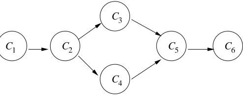
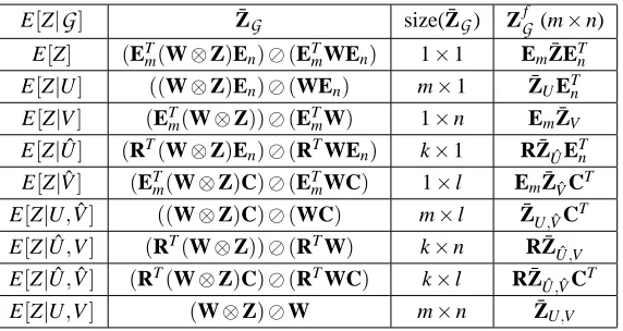
Figure 1 contains a graphical representation of the various co-clustering bases. For example, in Figure 1(a), the expectations along the row clusters (E[Z|Uˆ]) and the column clusters (E[Z|Vˆ]) are the statistics used for reconstructing the original Z. From the table, we can see that the various conditional expectations correspond to matrices of different sizes. We make use of this observation later in Appendix E to obtain a computational recipe for the Bregman co-clustering problem. The sets
C
1,C
2,C
5 andC
6 are symmetric in the row and column random variables whereasC
3 andC
4 are not. Further, if we have access to{E[Z|G
]:G
∈C
i}, for some 1≤i≤6, then we can compute{E[Z|
G
]:G
∈C
j} for all 1≤ j≤i, i6=4,j6=3. In this sense, we say that the constraint setC
iis more complex than
C
j for all j<i≤6,i6=4,j6=3 as illustrated in Figure 2. From a practicalperspective, a more complex set of constraints allows us to retain more information about Z, but obviously requires an increased number of parameters.
Our abstraction allows us to handle all the above schemes in a systematic way. Now, consider a co-clustering basis
C
∈ {C
i}6i=1as the pertinent one. Given the choice of a particular basis, weneed to decide on the “best” reconstruction ˆZ for a given co-clustering(ρ,γ). Then the general co-clustering problem will effectively reduce to one of finding an optimal co-co-clustering(ρ∗,γ∗)whose reconstruction has the lowest approximation error with respect to the original Z.
C
C C
C
C
C1 2
3
4
5 6
Figure 2: Relative complexity of the 6 co-clustering bases.
4.2 Minimum Bregman Information (MBI) Approximation
As in Section 3.1, for a given co-clustering (ρ,γ) and a given co-clustering basis
C
, we use the MBI principle to obtain the “best” approximation ˆZ. Recall that for block average co-clustering, the search for the MBI solution was restricted to all Z0 that preserved the co-cluster means. For a general co-clustering basisC
, the search space has to be appropriately generalized (or restricted) such that Z0 preserves all the summary statistics relevant toC
. LetS
A denote a class of randomvariables such that every Z0in the class satisfies the following linear constraints, that is,
S
A={Z0|E[Z|G
] =E[Z0|G
],∀G
∈C
}. (17)The reader may wish to compare the above definition (17) to the more specific definition (7) that is applicable in the case of block co-clustering. It can be readily seen that (7) follows by assuming that the co-clustering basis
C
={{Uˆ,Vˆ}}.We now select the random variable ˆZA∈
S
A that has the minimum Bregman information as the“best” approximation, that is,
ˆ
ZA≡argmin Z0∈S
A
![Figure 1: Schematic diagram of the six co-clustering bases. In each case, the summary statisticsused for reconstruction (e.g., E[Z|U ˆ] and E[Z|V ˆ]) are expectations taken over the corre-sponding dotted regions (e.g., over all the columns and all the rows in the row clusterdetermined by Uˆ in case of E[Z|U ˆ]).](https://thumb-us.123doks.com/thumbv2/123dok_us/9835953.1969838/20.612.151.471.230.655/schematic-clustering-statisticsused-reconstruction-expectations-sponding-columns-clusterdetermined.webp)