Robot introspection through learned hidden Markov models

Fox, M. and Ghallab, M. and Infantes, G. and Long, D. (2006) Robot

introspection through learned hidden Markov models. Artificial Intelligence,

170 (2). pp. 59-113. ISSN 0004-3702

http://eprints.cdlr.strath.ac.uk/2772/

This is an author-produced version of a paper published in

Artificial

Intelligence

ISSN

0004-3702

.

This version has been peer-reviewed, but does not include the

final publisher proof corrections, published layout, or pagination.

Strathprints is designed to allow users to access the research

output of the University of Strathclyde. Copyright © and Moral

Rights for the papers on this site are retained by the individual

authors and/or other copyright owners. Users may download

and/or print one copy of any article(s) in Strathprints to facilitate

their private study or for non-commercial research. You may not

engage in further distribution of the material or use it for any

profitmaking activities or any commercial gain. You may freely

distribute the url (http://eprints.cdlr.strath.ac.uk) of the Strathprints

website.

Robot Introspection through Learned Hidden

Markov Models

Maria Fox

Malik Ghallab

Guillaume Infantes

Derek Long

a_{Department of Computer and Information Sciences, University of Strathclyde,}

26 Richmond Street, Glasgow, G1 1XH, UK

b_{LAAS-CNRS, 7 Avenue du Colonel Roche, 31500 Toulouse, France}

Abstract

In this paper we describe a machine learning approach for acquiring a model of a robot behaviour from raw sensor data. We are interested in automating the acquisition of be-havioural models to provide a robot with an introspective capability. We assume that the behaviour of a robot in achieving a task can be modelled as a finite stochastic state transition system.

Beginning with data recorded by a robot in the execution of a task, we use unsupervised learning techniques to estimate a hidden Markov model (HMM) that can be used both for predicting and explaining the behaviour of the robot in subsequent executions of the task. We demonstrate that it is feasible to automate the entire process of learning a high quality HMM from the data recorded by the robot during execution of its task.

The learned HMM can be used both for monitoring and controlling the behaviour of the robot. The ultimate purpose of our work is to learn models for the full set of tasks associated with a given problem domain, and to integrate these models with a generative task planner. We want to show that these models can be used successfully in controlling the execution of a plan. However, this paper does not develop the planning and control aspects of our work, focussing instead on the learning methodology and the evaluation of a learned model. The essential property of the models we seek to construct is that the most probable trajectory through a model, given the observations made by the robot, accurately diagnoses, or ex-plains, the behaviour that the robot actually performed when making these observations. In the work reported here we consider a navigation task. We explain the learning process, the experimental setup and the structure of the resulting learned behavioural models. We then evaluate the extent to which explanations proposed by the learned models accord with a human observer’s interpretation of the behaviour exhibited by the robot in its execution of the task.

1 Introduction

The goal of the work described in this paper is to automate the process of learning how a given robot executes a task in a particular class of dynamic environments. We want to learn an abstract model of the behaviour of the robot when executing its task solely on the basis of the sensed data that the robot records when performing the task. Having learned an execution model of this task we want to use the model to reliably predict and explain the behaviour of the robot carrying out that same task in any other environment belonging to the class. This paper describes how we have approached this goal in the context of an indoor navigation task, and how successful we have been in learning a reliable behavioural model.

1.1 Motivation

The work presented here illustrates that it can be advantageous to approach a com-plex artifact, such as an autonomous robot, not from the usual viewpoint in robotics of the designer, but from the observer’s point of view. Instead of the typical engi-neering question of “how do I design my robot to behave according to some spec-ifications”, here we address the different issue of “how do I model the observed behavior of my robot”, ignoring, in this process, the intricacy of its design.

It may sound strange for a roboticist to engage in observing and modelling what a robot is doing, since this should be inferrable from the roboticist’s own design. However, a modular design of a complex artifact develops only local models which are combined on the basis of some composition principle of these models; it seldom provides global behavior models. The design usually relies on some reasonable as-sumptions about the environment and does not model explicitly a changing, open-ended environment with human interaction. Hence, a precise observation model of a robot behavior in a varying and open environment can be essential for understand-ing how the robot operates within that environment.

designing and modelling sensory-motor functions are necessarily too detailed. They are far too complex to be dealt with at a planning level, or even for execution mon-itoring. The latter requires intermediate level models, either hand-programmed, learned, or refined through specification and learning.

Other authors have considered how intermediate level descriptions of task execu-tion might be used for designing a robot, i.e., how the corresponding models might be encoded and exploited within a plan execution framework. We are not concerned with programming the low level control of the robot but with providing the means by which a robot can introspect about the development of its behaviour in the execu-tion of a task. We rely on hidden Markov models (HMMs) [25] as the intermediate level representation of this behaviour. Since these models are built empirically, they take into account the dynamics and uncertainty of the real execution environment. The resulting behavioural models provide a way in which the controller can reason about the robot behaviour in the context of executing a task.

Our focus here is not on learning topological or metric maps for robot navigation. Others have considered this problem in depth [1–4] and shown that navigation with respect to a given environment can be dynamically improved as the robot interacts with its environment. The use of stochastic learning techniques to improve robot navigation in a given environment is therefore quite well-understood. We are con-cerned with learning abstract models of how a robot performs a compound task, whatever that task might be. Navigation is an example of such a compound task.

1.2 Approach

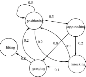
Our objective is to be able to predict and explain the robot’s behaviour as it un-dertakes a compound task in the uncertain real world. In reality the robot passes through a number of abstract behavioural states, some of which can be distin-guished and identified by a human observer. For example, when picking up an object in its grippers a robot might be in the state of positioning with respect to the object, approaching it, grasping it, knocking into it, lifting it, and so on.

To illustrate the kind of model we are interested in learning, figure 1 shows a high level state transition model of a pickup task (this is an artificially simplified example that was not learned from real data). Time is abstracted out of the model and it is assumed that a monitoring process tracks how often the robot revisits the same state.

fol-grasping

knocking approaching

lifting

positioning

0.2 0.8

0.9

0.1 0.8

0.2 0.5

0.3

0.2

Fig. 1. The compound task of picking up an object.

lowed by the robot might revisit the positioning state multiply often and it might be that the state of knocking into the object is entered most frequently when this is the case. Using the HMM to identify the most probable trajectory leading out of the current state provides a monitoring system with a powerful ability to determine the most likely outcome of the robot’s current behaviour. In section 7 we discuss how the structure of the HMM can be exploited by such a monitoring system.

The behavioural states of the model are hidden, because they cannot be sensed directly by the robot. The robot is equipped with noisy sensors from which it can obtain only an estimate of its state. A hidden Markov model (HMM) represents the association between these noisy sensor readings and the possible behavioural states of the system, as well as the probabilities of transitioning between pairs of states. The HMM is therefore ideally suited to our objectives. Our approach is to learn a HMM that relates the sensor readings made by the robot to the hidden real states it traverses when executing its task, in order to equip the robot with the capacity to monitor its progress during subsequent executions of the same task.

Our work makes several innovations. First, we address the problem of learning the structure as well as the parameters of the HMM, using a structural learning ap-proach based on Kohonen network clustering. We begin with no prior knowledge about how many states the HMM will have, or what the relationship between states and observations might be. Second, we learn an HMM that is independent of the physical locations at which activity takes place. The states we are concerned with are abstractions of the behavioural states of the robot. Expectation Maximization (EM) [5] is used to estimate the transition probabilities between them based on multiple sequences of robot observations, each sequence corresponding to the ob-servations made by the robot during an execution of the compound task.

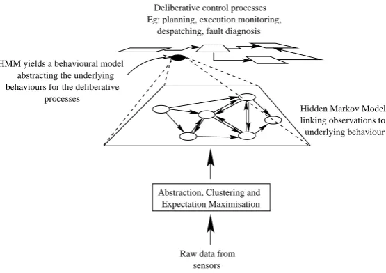
Figure 2 gives an overview of the whole learning process, and suggests how the resulting model might feed into high level deliberative reasoning processes. In this paper we focus on the processing and clustering of raw sensor data leading to the construction of HMMs. As we discuss in Section 7, these models represent be-havioural abstractions that can be used by high level deliberative processes.

ap-Expectation Maximisation Abstraction, Clustering and

Raw data from sensors

Hidden Markov Model linking observations to underlying behaviour Deliberative control processes

Eg: planning, execution monitoring, despatching, fault diagnosis

HMM yields a behavioural model abstracting the underlying behaviours for the deliberative

processes

Fig. 2. Learning an HMM from the bottom up.

proach. Although some questions remain to be answered we believe that our work constitutes an interesting step towards the acquisition of a predictive and explana-tory model of robot behaviour that is grounded in its actual sensed experience in reality.

1.3 Related Work

The work described in this paper builds on a varied literature concerned with the automated construction of stochastic behavioural models. This includes work on probabilistic plan recognition [6,7], learning topological and metric maps [1,2], learning stochastic models of human activity [8–13] and learning to recognise facial expressions [10] and gestures [14,11,13]. Previous authors have also considered the automatic classification and interpretation of sensed data [15] and the refinement of behavioural states to introduce previously unaccounted-for distinctions into a world model [2,16]. Our work therefore combines a number of established approaches in the acquisition of stochastic task models.

to adding states to the POMDP. The learned POMDP is therefore as accurate as possible a representation of a physical space.

Although the work is superficially related to ours, because EM is used to estimate the parameters of a stochastic model, its objectives are very different. Koenig and Simmons are specifically interested in learning to improve the navigation capability of a robot within a given environment, whilst we are interested in learning how a robot accomplishes a task, whatever the task may be. In the work we describe in this paper we use the navigation task simply as an example of a compound task. The states of our learned model correspond to abstract behavioural states, such as obstacle avoidance, not to physically grounded states such as one metre from a corridor junction. This is a significant difference because our method is task-independent. The states are acquired automatically by means of the clustering of sensor input and their veracity is established by evaluating the predictive power of the resulting HMM.

Several authors have considered how intermediate level models might be used for describing the execution of a task. For example, RAPS [19] and Structured Reactive Controllers [20] provide the low level programs into which actions at the task-planning level decompose at the executive level of the robot architecture. RMPL [21] and TDL [22] are examples of languages that have been developed for the specification of such programs. These programs might be hand-coded or they might be acquired by learning or by interpretation of learned models. The Proce-dural Reasoning System (PRS) [23] is a further example of an architecture that supports the relationship between high level plans and execution.

The work done in gesture [14,11,13] and facial expressions [10] recognition is closely related to our concern. If an HMM is used to model the probabilities of a human face transitioning between different expressions, and these expressions are linked to emotional states and actions, it becomes possible to predict the most likely next action of a person based on interpretation of his facial expression. Similarly, if gestures are associated with activities a learned HMM can enable the immediate goals of a person to be predicted on the basis of his recent and current gestures. This work is similar to our own because the states of the learned HMMs are behavioural states of the subject and are not associated with the physical location of the subject.

activities that typically take place at these locations. Thus, the work is concerned with relating activities to physical space and its emphasis is therefore different from our own.

In our work the association between the sensor readings of the robot and its be-havioural states is learned by means of Kohonen network clustering. A closely related approach in the literature is the work of Oates, Schmill and Cohen [15] in which dynamic time warping is used to cluster multivariate time series sensor data, or experiences. Oates et al. present an unsupervised method of clustering experi-ences into classifications of action outcomes enabling a robot to interpret its state in a way that accords well with human judgements. The objective of their work is to identify cluster prototypes that form the basis of an ontology of activity that can lead to the automated construction of operator models. The way in which we use the results of the clustering phase is different and a more detailed comparison follows later in the paper.

1.4 Layout of the Paper

In section 2 we formulate the problem we are addressing, specifying the notation we will use in this paper, introducing the main methods and algorithms and defin-ing the key terms that we will use. In section 3 we discuss data clusterdefin-ing usdefin-ing the Kohonen network clustering approach. We describe how an initial collection of behavioural states is refined by the clustering process. We then explain the pro-cess of building an initial sensor model using the code book approach, and show how all of the remaining parameters of the HMM are initialised. We then review EM, describing how the initial parameters are iteratively reestimated. Section 4 de-scribes the robot and its array of sensors, the data we collected and the class of environments we studied. We explain how the observable outputs of the robot are processed to extract the features used for clustering, and how the feature vectors we used are constructed. In section 5 we discuss the implementation of the entire learning process, showing how the EM process was integrated with the clustering phase in our system. The EM process requires evidence to be provided, and we explain how sequences of observations are generated for this purpose.

In section 6 we describe the evaluation strategy we have devised for determining the quality of the learned HMM in terms of its power to explain the robot’s be-haviour from its observations. Using the Viterbi algorithm [24] we construct the sequences of states that best explain the observation sequences, and then we com-pare the Viterbi sequences with what the robot did in reality. This comparison relies on a human observer’s interpretation of the robot’s real behaviour. We discuss the strengths and weaknesses of this approach.

in the monitoring and control of robot behaviour. Although this is not the focus of the current paper we explain how the HMMs can enable a robot to predict entry into an undesired state and to take averting action in time to avoid a failure. We discuss how HMMs can be used in combination with policies and plans to support a robot in achieving high level mission goals.

2 Formal Problem Statement

There are three main problem components to define: the model of a task as a finite state transition system, the clustering of the observation space into a finite evidence space, and the definition of the finite behaviour state space. For each component we will present the assumptions that we make concerning the component and its role in the problem, the formal definition of the component and a brief introduction to the algorithm that is used to construct instances of the component. In the following section we present details of the core algorithms introduced here.

In our definitions we usen andm as index variables indicating the lengths of

se-quences in the context of each definition. These variables should be interpreted as locally defined within the scope of each definition.

2.1 Models and Tasks

Assumption: The robot behaviour for task T can be conveniently modelled by a

finite stochastic model.

Definition 1 A stochastic state transition model is a 5-tuple, λ = (Ψ, ξ, π, δ, θ), with:

• Ψ ={s1, s2, . . . , sn}, a finite set of states;

• ξ={e1, e2, . . . , em}, a finite set of evidence items;

• π: Ψ→[0,1], the prior probability distributions overΨ;

• δ : Ψ2 _{→ [0,1], the transition model ofλsuch thatδ}

i,j =P rob[qt+1 = sj|qt = si]is the probability of transitioning from state si to statesj at time t (qtis the actual state at timet);

• θ : Ψ ×ξ → [0,1], the sensor model ofλ such that θi,k = P rob[ek|si] is the probability of seeing evidenceekin statesi.

Under the Markov assumption the state of the robot at timet depends only on its

state at timet−1, so thatλproduces a hidden Markov model.

The algorithm we are using to build the model is the well-known technique of Ex-pectation Maximization (EM) [25], also called the Baum-Welch algorithm [26]. Given a set of histories and the initial parameters of a HMM — an initial sensor model, an initial transition model and a prior state distribution over the states in

Ψ— EM iteratively reestimates the HMM parameters. On each iteration EM

es-timates the probability, or likelihood, of the evidence being seen given the HMM estimated so far. It then updates the model parameters to best account for the evi-dence. When the estimated likelihoods are no longer increasing EM converges. The probability at convergence is represented as the maximal log likelihood: the best lo-cal estimate possible given the evidence and the learned model. Log likelihood is used because the probability of a particular observation sequence being seen in a complex model is typically low enough to challenge the arithmetic precision of the machine. It is well-known that EM has a tendency to converge on local maxima, but careful selection of the initial HMM parameters can help to mitigate this tendency.

The inputs to the EM algorithm are: a finite set of histories, H = {h1, . . . hn},

corresponding to the training data associated withn executions of task T, and an

initial model, λ0 = (Ψ, ξ, π, δ0, θ0). The output is a learned stochastic model λ

corresponding to a hidden Markov model describing the taskT.

2.2 Clustering the observation space into evidence

Assumption: A multi-dimensional non-finite observation space can meaningfully

be mapped into a finite set of evidence items.

We refer to the collection of sensor readings that can be made by the robot, at some point in time, as an observation. Each reading gives the value of a certain primitive feature which we call a raw feature, such as the heading of the robot, the speed at which it is travelling, and so on. The observation space is therefore defined by the particular collection of sensors with which the robot is equipped and its interaction, by means of these sensors, with the environment.

Definition 3 A k-dimensional observation space is defined asΦ =γ1×γ2×. . .×γk, where:

• γi ⊆ <;

• A raw feature is defined to be a functionfi :robot×env×time→γi mapping

the sensory-motor and environmental context of the robot, at a timet, to a value

in the rangeγi, thus partially characterising the behaviour of the robot at some instanttin time.

Definition 4 An observation is a point in observation space.

access to this function or control over how it produces its mapping to raw feature values. Raw feature values are determined by the low level robot control software upon which the learning pursued in this project is based and the interaction between the robot and its environment. We can samplefifor specific values of its arguments.

Under our assumption mappings exist from the observation space Φ to a set of

abstract observationsξ. We call the elements ofξevidence items. We first define a trajectory, then explain how the construction of trajectories allows the setξ and a mapping to be constructed by means of the clustering of the observation space.

Definition 5 A trajectoryτ = ho1, o2, . . . , oniis a finite sequence of observations characterising a single execution of the taskT.

Our intention is to discretise the non-finite observations, Φ, of the robot into a

finite collection of distinct evidence items, ξ, and to determine a mapping

clus-ter : Φ → ξ. This requires a process of abstraction and the combination of raw

feature values across observations. A single observation is not informative enough to enable us to determine how the robot’s behaviour develops over time. If we

con-sider a single observation taken at time t the raw feature values will reveal very

little about how the robot’s behaviour has evolved up to that time, or will evolve af-ter it. For example, because the robot is reacting to its environment the observation

it makes at timet might record a heading several degrees away from the general

direction in which the robot travelled over an interval includingt. We are less in-terested in the precise heading at time tthan in the general direction in which the robot travelled over a period of time that includest.

In order to see how the behaviour of the robot changed over time we consider

sub-sequences of trajectories, each containing c consecutive observations, where

c is a constant chosen to ensure that the sequences represent sufficient time for

interesting behaviour to occur. We combine the raw feature values associated with observations in these sequences into features, then focus on how the values of the features in which we are interested vary over different sequences.

Definition 6 For a given constantc, a feature is an abstraction of raw feature

val-ues, obtained by combining some subset of the raw features drawn from each ofc

consecutive observations.

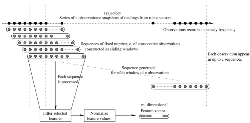
The combinations performed in definition 6 are typical filtering and smoothing operations used in signal processing. Using features we construct feature vectors from the trajectories in our data set.

Definition 7 A feature vectorf~i is anm-dimensional vector of feature values. The feature values are obtained from a sub-sequence of a fixed number of consecutive observations, starting at observationi, in a trajectory.

obser-Filter selected features

Normalise feature values

Feature vector is processed

Observations recorded at steady frequency Trajectory

constructed as sliding windows

Each observation appears

Each sequence

Sequence generated

Sequences of fixed number, c, of consecutive observations

for each window of c observations

in up to c sequences

m−dimensional Series of n observations: snapshots of readings from robot sensors

Fig. 3. Sliding window construction of feature vectors

vation space that isk-dimensional where, in general,m ≤kdepending on the ways

in which the raw features are combined in the construction of the features.

The feature vectors are constructed in the following way. For each trajectory we take all possible consecutive sequences of a fixed number of observations using a typical sliding window approach as shown in figure 3.

We do not allow feature vectors to cross the boundaries between trajectories. This helps the system to learn that the robot never transitions out of the state in which it has reached its goal into any other state.

Before clustering we normalise the feature vectors to ensure that variation in vector magnitude does not distort the clustering results. We also normalise each field of the feature vectors by expressing each value in terms of the number of standard deviations from the mean value for that field. This ensures that gross differences in the ranges of values do not get interpreted as magnitude differences by the clusterer.

The algorithm we use for clustering the observation space is Kohonen network clustering. The Kohonen network performs an unsupervised projection of multi-dimensional data onto a smaller multi-dimensional space, resulting in the identification of a cluster landscape in this smaller dimensional space.

We chose to use the Kohonen self-organising network because it gives us the free-dom to avoid specifying the number of clusters in advance. We first train the net-work and then apply a cluster selection function to the landscape to identify the most significant clusters. Thus, although the size of the network places an upper bound on the number of clusters that can be found, there is no need to predetermine how many clusters the data set contains. In vector quantisation approaches [27],

determines the number of clusters that will be found. Similarly, in stochastic clus-tering using techniques such as EM, the user must supply the number of Gaussians to use in a mixture, which determines the number of clusters that will be learned. In our application it is important that the number of evidence items be determined autonomously from the structure of the observation data, since we do not wish to impose any prior judgements on what observations the robot might be making. Fur-thermore, the self-organising network has the useful property that clusters that are close together in the network map to concepts that are close in reality. We exploit this property by using scalar product operations to identify relationships between evidence items and behavioural states. We describe this process in section 3.2.

The input to the clustering process is a finite set of feature vectors constructed

from the trajectories. The outputs are the set of evidence itemsξand the mapping

cluster :Φ→ξ. Using the cluster mapping we can construct the set of historiesH.

2.3 Defining the State SpaceΨ

Assumption: It is possible to determine a priori a collection of behavioural states

associated with a taskT.

We distinguish between states that are unambiguously visible to the observer, such ass0, the starting state, sg, the finishing state andsf, failure states, and those that must be identified subjectively, such as hesitating. These we denote the subjective states. The refinement process replaces the subjective states (and, optionally, the visible states), with other hidden states, unknown to the human observer.

A human observer can label observations while the robot is performingT. The

la-bels are associated with the observations as they occur in real time. The labelling indicates the association between an observation and a behavioural state, as per-ceived by the human observer. The set of labels therefore corresponds to the a priori state set. We call the set of labels used by the human observerL.

GivenLwe can define a partial labelling of trajectories by the human operator.

Definition 8 A partial labelling maps a trajectoryτ =ho1, o2, . . . , onito a labelled trajectoryτ0 =h(o1, l1),(o2, l2), . . . ,(on, ln)i, where:

• oi ∈Φ;

• li ∈ L∪ {nomark}, wherenomark is the label applied to an otherwise unla-belled observation.

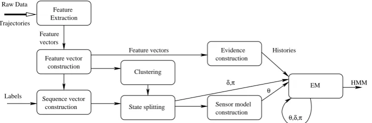
Sequence vector construction Feature vector

construction

Evidence construction Clustering

State splitting Sensor model construction

EM Extraction

Feature

Labels

Feature vectors Histories

δ,π

θ HMM

θ,δ,π

Feature vectors Trajectories

Raw Data

Fig. 4. Learning an HMM from raw sensor data. The bold arrows show the input to and output from the entire learning process.

finding the maximal cliques in a graph in which the nodes correspond to evidence items in ξ. A separate graph is constructed for each of the state labels in L. The structure of the graph is determined by the cluster mapping. An edge is constructed between nodeseiandej if cos−1(ei·ej)≤ρwhereρis a constant threshold angle between vectors in the feature vector space,ξ. Each maximal clique, corresponding to a subset of evidence items inξ, is interpreted as a state inΨ. The elements ofΨ

are substates of the label setL∪ {nomark}.

The inputs to the maximal clique finding algorithm are: the set of labels L, a set of partially labelled trajectories, the set of evidence itemsξ, and the mapping clus-ter :Φ →ξ. The output is a setΨof states, which we take to be the state space of the taskT.

3 The Core Algorithms

We now describe the three main algorithmic components of the system in more de-tail, showing how they construct the components described in section 2. We present these algorithms and components in a way that is independent of the specific task, environment and robot platform that we considered. Our objective is to emphasise the generality of the approach we have taken. In the next section we explain how the data we used was collected and prepared for presentation to the system.

3.1 Kohonen Network Clustering

As stated in section 2.2, the input to the clustering process is a set of feature vectors constructed by smoothing trajectories over intervals of time. The outputs are the set of evidence items,ξand the mapping cluster :Φ→ξ.

3.1.1 The Clustering Process

We performed clustering using a two-dimensional self-organising map, or Kohonen network [28]. The Kohonen network identifies patterns in feature vector data in a way that is independent of human influence. The number of clusters found depends purely on the form of the data itself and the parameters of the network. The param-eters are the dimension of the network (we used a square grid), the learning rate, the neighbourhood size and the random number seed used to initialise the network vectors. This independence is important because we have no way of deciding a pri-ori how many observations the raw data contains or what their relationship to one another might be.

Kohonen clustering performs a projection of n-dimensional data onto a smaller,

k-dimensional, space, where k is less thann and can be determined by the user.

We use k = 2, so we are projecting the multi-dimensional structure of our data

onto a 2-dimensional space. Within this framework the dimension of the network affects how many clusters are found and how they inter-relate. The dimensions of the network should be at least 500 times smaller than the size of the data set [28] to allow for enough space for clusters to be distinguished, but not so much that that they begin to degenerate into noise. Our data set consists of about 15,000 feature vectors so we experimented with dimensions varying between 15 and 45. Increas-ing beyond a dimension of about 35 seems to increase the amount of noise in the cluster landscape, which has a negative effect on the quality of the learned HMM. Using a dimension below about 20 causes clusters to combine and reduces the level of discrimination, again resulting in a negative effect on learning. Networks of di-mension between 25 and 30 seems to give the best results for our data set, as we demonstrate in section 6 and appendix B.

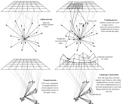
The map is initialised with random unit vectors of appropriate dimension. We ini-tialised the network using random vectors that cover the network adequately (we insist that all of the initial vectors must be pairwise separated by at leastddegrees, wheredis a constant chosen depending on the size of the network). This is to reduce the effects of initial bias in the network. Initial bias is a widely recognized problem in the use of clustering algorithms. All our results are presented as averages over 20 random number seeds, as discussed in section 6.

multi-Identify closest cell vector to input vector; move all vectors in cells in

neighbourhood of closest vector towards the input.

Training process

moved towards Neighbours

input contains random

vector Each cell

Initial network

Cell vectors organised closely aligned vectors representing clusters in in neighbourhoods of

the input vectors

Trained network

Neighbourhood

Landscape generated by counts

Landscape Construction

Sort cells and select cell with highest count. Remove cells within

neighbourhood of newly selected cell, where neighbourhood size is inversely proportional to cell count.

Repeat until all cells selected or removed. Neigbourhood

Input

Closest cell

Fig. 5. Training the Kohonen network

plication is used to determine closeness. Alignment is performed by adding to the network vector a proportion of the sequence vector as determined by the learning rate. A neighbourhood value determines the neighbourhood of network vectors that is influenced by the input feature vector. We implemented a neighbourhood decay rate as a negative exponential function. The effect that this has is to reduce the impact of training vectors over time. Using this function we can iterate over the training data many times without over-learning. We also used a learning rate decay, in the form of MacQueen’s averaging law [29]. Thus, in a way determined by the learning rate and neighbourhood value chosen, the 2-dimensional space partitions into regions.

different robot behaviours in the data set. Each trajectory produces fewer examples of the smoothed observations associated with the starting and finishing behaviours of the robot, than examples of observations associated with the intermediate be-haviours. Experiments showed that shuffling more frequently led to the network failing to distinguish the starting and finishing observations from observations as-sociated with the intermediate behaviours.

After training the 2-dimensional space can be mapped to a vector space of dim2

vectors, wheredimis the dimension of the network. In order to identify the clusters in this vector space we apply an cluster selection strategy to the network which draws the vectors together around the highest peaks. Our first attempt at such a strategy counted, given a cell hi, ji, the number of cells that were within a fixed radius (we used 0.085) of hi, ji. This count was used to measure the influence of

hi, ji over the whole network. We then used a hill-climbing strategy to associate plateau cells with the first closest peak found.

There are several weaknesses associated with this approach. The first is that, using this strategy, the composition of the peaks ends up very sensitive to the noisiness of the cells in the network. We noticed that, with different random initialisations, we got very different cluster landscapes. A cell might be pulled one way or the other depending on random factors, so that a small change in the initialisation of the net-work could lead to huge differences in the cluster landscape. Large variations make the later learning results highly dependent on arbitrarily chosen random numbers.

Another weakness is that the cells exerting the most influence in these terms over the network are not necessarily the cells that attracted most of the input during training. Using this method we could end up throwing out the clusters we are really interested in in favour of ones that attracted little input and are not good indicators of the behaviour of the robot. Further, by associating the cells in a plateau with the nearest peak we caused the network to distort, sometimes very badly in the cases where there are large plateaus. A better approach seems to be to restrict the amount of draw that one cell can have over another, and thereby spread the clusters more evenly over the landscape.

To address these problems we developed a different cluster selection strategy which uses the number of inputs attracted to each cell as a way of identifying the cluster landscape. The cells that attracted the most inputs we take to be the highest peaks in the landscape. Given that the cluster landscape is intended to represent the structure in the data set we decided that a cell that attracts very few inputs is unlikely to be interesting, so we focus our attention on the high peaks. To achieve this focus we associate a varying neighbourhood size with the peaks in the network, considering the peaks in descending height order. This neighbourhood is different from the learning neighbourhood used during training.

0 5

10 15

20 25

30 0 5

10 15 20 25

30 0

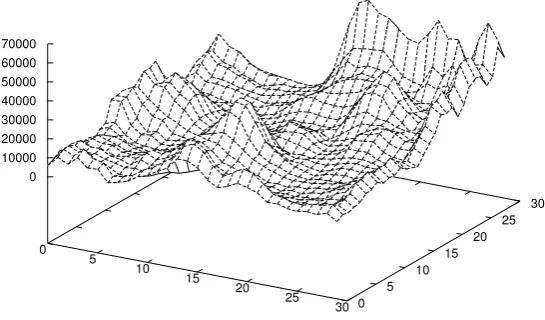
10000 20000 30000 40000 50000 60000 70000

Fig. 6. A clustering landscape obtained using a 30x30 Kohonen network.

all of the cells in its neighbourhood. The size of the neighbourhood is determined as:

&

H C

'

whereHis the number of inputs attracted to the highest overall peak in the network andC is the number of inputs attracted to the current peak. This value is used as a radius around the peak cell. The process is repeated for the next highest peak until no cells remain to be considered.

LetCbe the current peak andH be the height of the highest peak in the network.

Clearly, if H_C is large for most values ofCthen we risk losing the interesting struc-ture in the network. This is obviously undesirable, resulting in a small collection of clusters that is unlikely to be discriminating. We require the value of H_C to have a slow, smooth gradient over a sufficiently large collection of discriminating clusters. For the size of our data set sufficiently large means tens of clusters. To achieve such a gradient we require the ratio ofHtoCto be small for tens ofCs. By examining the cluster landscapes constructed from our data set we confirmed that this require-ment is satisfied. Figure 6 gives an example of a typical cluster landscape generated using a network of size 30.

We have found that using this strategy we improve the clustering stability by re-ducing sensitivity to the noisiness of the randomly generated vectors. Peaks still move around in the network because of the random initialisation, but this is to be expected. The experiments presented in section 6.4 show that we achieve a high degree of stability in the clustering results across different random number initiali-sations.

classi-fication. During classification, each input sequence vector is associated with the peak vector to which it is closest according to a scalar multiplication comparison between the feature vector and each peak vector. The cells in the network that cor-respond to the peaks contain vectors that characterize the evidence items found by

the clustering process. These are the elements of the set ξ and correspond to the

evidence items that can be observed by the robot as it executes its task. We refer to these vectors as characteristic vectors.

Our clustering approach is related to that of Oates et al. [15] who considered the problem of clustering the experiences of a robot into qualitatively different action outcomes. Their cluster prototypes, which are closely related to our characteris-tic vectors, constitute an ontology of activity. It is intended that they correspond to the qualitatively different states in which a robot can find itself, following the execution of an action, and that they provide the basis for automating the descrip-tion of acdescrip-tions at the task-planning level. By contrast, our characteristic vectors are interpreted as high level observations, or evidence items, associated with states at the intermediate level of description rather than at the task-planning level. As we will see, observations contribute to the identification of states, at this intermediate level, which might have no interpretation for the human observer but which may be critical in accurately modelling the behaviour of the robot with respect to its task.

At the end of the classification phase all of the feature vectors in our data set have been classified with one of the characteristic vectors in the network. This puts us in a position to construct an observation code book.

3.1.2 Constructing the Sensor Model

A code book [27] is a mapping from input values to a finite collection of obser-vation codes. To build our code book it is necessary to associate the characteristic vectors with the labels in L∪ {nomark}. To facilitate this we annotate each fea-ture vector with the label associated with the last observation in the sliding window from which the feature vector was constructed. If there are no labelled observations in this sliding window the feature vector is labelled no mark.

The association of a feature vector with a label results in a new structure which we call a sequence vector. The structure of a sequence vector is defined in definition 9.

Definition 9 A sequence vector sv = (f~i, l) is an m-dimensional feature vector associated with a label,l, from the setL, taken from the last labelled observation in the sub-sequence of the partially labelled trajectory from whichf~iwas constructed. If there are no labels in the subsequence thenlis the no mark label.

Kohonen network.

Definition 10 Given a trajectory t = ho1, . . . , oni, the ladder lt is the sequence

{f~1, . . . , ~fn}of sequence vectors constructed from trajectoryt.

The sequence vector construction phase defines a mapping from trajectories to lad-ders, defined in definition 10, so-called because of the way that the sequence vectors overlap in a sliding window, as shown in figure 3.

We can now construct the association between evidence items inξ and the labels

inL∪ {nomark}by counting the number of sequence vectors carrying each label, the feature vectors of which were classified with each evidence item. This associ-ation can be turned into a probabilistic observassoci-ation function in the following way. Let s0, . . . , sn be the behavioural states labelled by L and e0, . . . , em be the evi-dence items. We interpret the number of associations in a given pair (si,ej) as a proportion, so that the probability of seeing evidence ej in state si can be easily calculated. LetVj_si be the set of sequence vectors associated with evidence itemej that were labelled withsi, andVsi be the set of sequence vectors labelledsi. Now

the probability of seeing evidenceej in statesi is:

θi(j) =

|Vj_si|

|Vsi|

The resulting function can be interpreted as a sensor model specifying the proba-bility of seeing each evidence item given each state. The “sensor” is the compound sensor capable of observing the evidence items found by the clusterer. This means that when subsequently using the model the robot’s raw sensor data can be pro-cessed by the construction of sequence vectors and their classification by means of cluster :Φ→ξ.

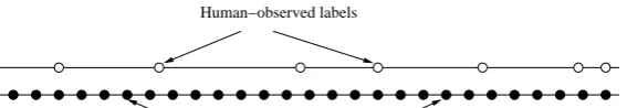
In section 6 we present results showing the quality of HMMs learned on the basis of sensor models constructed in this way and not further refined by state splitting. As can be seen from figure 19, the quality of the HMMs learned on this basis is often poor. We hypothesised that the states identified by the human observer might not in fact be the states that are most important for distinguishing between the be-haviours of the robot, and that better results might be obtained by sub-dividing the

human-observed labels. The labels inL∪ {nomark}abstract out a great deal of

3.2 Maximal Cliques

As stated in section 2.3, the inputs to the maximal clique finding algorithm are the set of labelsL, a set of partially labelled trajectories, the set of evidence items and cluster :Φ→ξ. The output is the set of statesΨ.

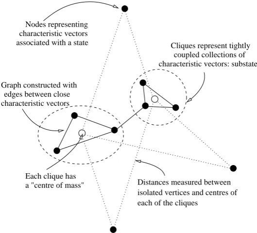
In the code book multiple evidence items can be associated with the same be-havioural state. This occurs because evidence items are not perfect discriminators between states. Sometimes, the characteristic vectors of these evidence items are separated in the vector space by significantly large angles. When these angles ex-ceed 30 or 40 degrees it seems plausible that the association of these clearly differ-ent evidence items with the same behavioural state might indicate that a decompo-sition of that behavioural state into sub-states is possible.

The idea of state-splitting around distant groups of characteristic vectors is illus-trated in figures 7 and 8. The procedure refineθ, in figure 7, begins by constructing, for each labels ∈ L, a graph in which the nodes are the characteristic vectors of the evidence items associated with that label in the code bookθ. The edges in the graph are the angles in vector space between the evidence items at the two end-points. If two vectors are less than a pre-determined threshold apart – for example, 40 degrees – an edge between their corresponding nodes is added to the graph and the maximal cliques remaining in the graph are found. These steps are illustrated in lines 6 to 15 of the constructGraph procedure.

The maximal cliques contain all those evidence items within 40 degrees of one another. Each maximum clique is a subset of the characteristic vectors associated with the original label, suggesting a substate of the behavioural state corresponding

to that label. The procedure refineθ shows how finding the maximal cliques leads

to the construction of a refined sensor model.

The sensor model, θ0_{, is constructed from the code book using the identified}

sub-states. We want to replace the original behavioural states labelled byL∪{nomark}

with their substates and to share out the association between an evidence item and

a label amongst all of the substates of that label. Thus: if evidence item e had a

1: Procedure: constructGraph(θ,s,ξ)

2: Input: code bookθ, label s, evidence itemsξ

3: Output: graph structure G 4:

5: initialise graph G 6: for all cluster c inξdo

7: if assoc(θ,s,c)>0 then 8: add node for c to G

9: end if

10: end for

11: for all (cluster) node i in G do 12: for all (cluster) node j in G do

13: if angle(i,j)<SEPARATION-THRESHOLD then 14: add edge (i,j) to G

15: end if

16: end for

17: end for 18: return G 19:

20: Procedure: refineθ(θ,L,ξ)

21: Input: code bookθ, labels L, evidence itemsξ

22: Output: sensor modelθ0 23:

24: initialise sensor modelθ0

25: for all label s in L do 26: G = constructGraph(θ,s,ξ)

27: {First identify the maximal cliques in G}

28: Cs = maxCliques(G)

29: initialise 2d array of doubles, ds 30: for all cliques clq in Cs do

31: {Find the mean of clusters representing nodes in clq}

32: avC = computeAverage(clq)

33: for all characteristic vectors c inξdo

34: {Record distance between centre of clique and characteristic vector c}

35: ds[clq][c] = scalarProduct(avC,c)

36: end for

37: normalise ds[clq] 38: for all cluster c inξdo

39: θ0[clq][c] = assoc(θ,s,c)/ds[clq][c]

40: end for

41: end for

42: end for 43: returnθ0

Distances measured between isolated vertices and centres of each of the cliques

Cliques represent tightly coupled collections of characteristic vectors: substates

Graph constructed with edges between close characteristic vectors

Each clique has a "centre of mass" associated with a state

characteristic vectors Nodes representing

Fig. 8. The state splitting procedure

of procedure refineθ. Figure 8 shows how this sharing is achieved.

As a result of the state splitting process the code book is rewritten in terms of the substates found. The number of evidence items does not change as a result of state splitting, but the number of states increases and is determined by the structure of the vector space following clustering. Interestingly, the states in the refined set have no interpretation for the human other than that they were obtained by decomposi-tion of an original set of human-observed labels. Nevertheless, some of the new states might represent interesting transitionary states that are important for learning a good state transition function and can therefore improve the results obtained from the EM phase.

The state collection that results from the refinement of the initial state labels is the state setΨ, and the sensor model, constructed using the relationship betweenΨand ξ, is the functionθ0_{. The relationship defines a function,ab : Ψ→L, which maps}

states inΨto labels in the initial collection (abindicates an abstraction step). We

also define a function ev : Ψ → _Pξ which, given a state inΨproduces the set of

evidence items that constitute it. The following property holds:

∀s1, s2 ∈Ψ·ab(s1) =ab(s2)⇒ev(s1)6=ev(s2)

which means that, if two states map byabto the same label, they will not contain

the same evidence items. We can also identify a mapping from labels to sets of substates which, given a label produces the set of substates in its decomposition.

We call this mapping refine :L∪ {nomark} →_PΨ.

same evidence items. Their association with different labels distinguishes them. However, the fact that two labels contain substates composed of identical evidence items can be taken to indicate a sharing of content between the two labels. Part of the power of the state-splitting procedure resides in its ability to identify the shared sub-structure of abstract states, as well as the characteristics that distinguish them. We explain in section 6 how the recognition of shared sub-structure can be exploited in the evaluation of the learned HMM.

The idea of decomposing and augmenting the states of a HMM has been considered by other authors [1,16]. In particular, Koenig and Simmons’ GROW-BW algorithm allows new states to be added to a HMM if they are needed to account for observa-tions made by a navigating robot. Chrisman [16] shows how dynamic partitioning of the state space of the model can overcome the problem of perceptual aliasing that occurs when a model contains too few states to discriminate between different observations. Stolcke and Omohundro [30] show how states can be dynamically merged to generalise a HMM. In these works the HMM starts with a collection of states that is determined a priori and is known to be inadequate to account for the observations of the system. State splitting and merging is applied during the learning process to increase the adequacy of the state set as observations are made.

By contrast, we propose a static state splitting strategy to be performed prior to the

EM learning process. Its purpose is to increase the information content ofλ0 _and

thereby improve the quality of the learned model. Indeed, the results we present in figure 19, section 6, demonstrate that the quality of models learned after state splitting is significantly higher than is obtained when state splitting is not used.

Once the state set of the HMM is decided it is never changed – only the next-state and observation probability distributions are affected by reestimation. The states to which the splitting algorithm is applied are the labels inL∪ {nomark}. Splitting allows these states to be refined so that transitionary states emerge and structure is made accessible that was not apparent to the human observer. It is intended that our state splitting algorithm identify a complete (with respect to the available sensors) set of the hidden states that accounts for the behaviour of the robot with respect to its task.

3.3 Expectation Maximisation

the need for scaling and the way in which scaling is performed when multiple his-tories are used in reestimation and, finally, the use of the learned HMM to diagnose the state of the system from a given history. In order to be self-contained, and to clarify our contribution, we summarise the main aspects of the EM technique.

In an EM implementation of reestimation there are two key steps: the E step, which is the calculation of the maximum likelihood of seeing the evidence given the model so far, and the M step, which is the process of updating the model to maximize the probability of seeing the evidence. The E step is performed using the so-called forward-backward algorithm, originally described in [31,32], and very clearly pre-sented by Rabiner.

The M step, in which the transition and sensor model components of the HMM are updated, is affected by the scaling of the values generated by the forward-backward algorithm. As Rabiner discusses, scaling is necessary in the E step to avoid under-flow. Without scaling, underflow occurs because the probability of seeing a long sequence of evidence is very small, so as the history lengths grow the E step cal-culations tend to zero. It is necessary to demonstrate that the scaled values do not change the interpretation of the update operations. This is straightforward to show when a single history is used for learning, but more subtle when multiple histories are used. In the work we describe in this paper, we used multiple histories because our data set contains multiple separate and independent trajectories. In appendix A we discuss how we implemented the scaling mechanism following Rabiner’s pre-sentation. In this section, we present the core components of the E and M steps, showing how scaling is managed in the case of multiple histories.

3.3.1 Basic framework

We begin by providing here some definitions from Rabiner’s tutorial that are nec-essary for our presentation. The forward and backward variables are defined below. The M step of the EM procedure, which performs the updating of the model, is defined in terms of the forward and backward variables. Definitions 11, 12, 13, 14 and equations 1 and 2 are taken from Rabiner’s paper.

Definition 11 Given a historyh = he1, e2, . . . , eTi, a collection of statesΨand a modelλ= (Ψ, ξ, π, δ, θ), the forward variableαt(i)is defined to be the probability of being in statesi at timet, having seen the first telements ofh, given the model λ. This is formalised as:

αt(i) = P(e1. . . et, qt =si|λ)

The forward variable is constructed recursively as follows:

Initialisation:

Induction:

αt+1(j) =

N X

i=t

αt(i)δ(i, j)θj(et+1),1≤t≤T −1,1≤j ≤N

Termination:

P(h|λ) =

N X

i=1

αT(i)

Definition 12 Given a historyh = he1, e2, . . . , eTi, a collection of statesΨand a modelλ= (Ψ, ξ, π, δ, θ), the backward variableβt(i)is defined to be the probabil-ity of seeing the lastT −telements ofh, given that the state of the system at timet issiand given the modelλ. This is formalised as:

βt(i) = P(et+1. . . eT|qt =si, λ)

The recursive construction of the backward variable is as follows:

Initialisation:

βT(i) = 1,1≤i≤N

Induction:

βt(i) = N X

j=1

δ(i, j)θj(et+1)βt+1(j), t=T −1, T −2, . . .1,1≤i≤N

With these variables we can now define the transition model and sensor model update components of the M step. The prior probability distribution,π, is not rees-timated if an unambiguous initial state can be identified for which the probability is 1. We assume that this is the case, and explain why in section 3.3.3. We begin with the basic transition model update. In the following, the primed notationδ0(i, j)and θ_j0(k)denotes the updated values ofδ(i, j)andθj(k)respectively.

Definition 13 The transition model componentδofλ is updated according to the following equation.

δ0(i, j) =

PT−1

t=1 αt(i)δ(i, j)θj(et+1)βt+1(j)

PT−1

t=1 αt(i)βt(i)

Definition 14 The sensor model componentθofλis updated by:

θ_j0(k) =

PT

t=1

s.t.et=k

αt(j)βt(j)

PT

t=1αt(j)βt(j)

Definition 14 states that the probability of observing evidence k while in state j

is given by the expected frequency of being in state j and observing evidencek,

divided by the expected frequency of being in statej.

We now turn to the scaling issue and its effect on these update equations. Thetth forward scaling term can be defined as the likelihood of seeing the firsttelements of the history and being in statei. This is expressed as:

Ct= Πtv=1cv

wherecv is the normalisation term:

1

PN

i=1αv(i)

Thet+ 1th backward scaling term can be defined as:

Dt+1 = ΠTv=t+1cv

The normalisation term cv is calculated during the E step. The update equations

definingδ0(i, j)andθ0_j(k)can be rewritten to incorporate these scaling terms in the M step. Equation 1 shows how the transition model update is modified.

δ0(i, j) =

PT−1

t=1 Ctαt(i)δ(i, j)θj(et+1)Dt+1βt+1(j)

PT−1 t=1

PN

j=1Ctαt(i)δ(i, j)θj(et+1)Dt+1βt+1(i)

(1)

The variablesαt(i)andβt(i)are scaled by multiplying them byCtandDt respec-tively. The scaled forms are written using the notationαˆandβˆ. Thus:

Ctαt(i) = ˆαt(i)

and

Dtβt(i) = ˆβt(i)

The sensor model update θ0_j(k) can be modified in a similar way. Rabiner shows that the terms CtDt+1 can be expressed in a form independent of t, so that they

3.3.2 Scaling with multiple sequences

Rabiner discusses the fact that, depending on the kind of HMM being learned, there may be a need to learn using multiple histories in preference to one long sequence of evidence. In this case, it is necessary to modify the reestimation formulas to add together the individual frequencies of occurrence of each sequence. Before

this sum, the expected frequency of transitions from itoj in sequencek must be

scaled by dividing it by the likelihood of sequencekgiven the model. The expected frequency of stateiin sequencekmust also be divided by this likelihood. IfPk is

the likelihood of sequencek this can be achieved by multiplying the contributions

made by this sequence to both the numerator and denominator by _P1

k.

δ0(i, j) =

PK k=1

1

Pk

PTk−1

t=1 αkt(i)δ(i, j)θj(ekt+1)βtk+1(j)

PK k=1

1

Pk

PT−1

t=1 αkt(i)βtk(i)

(2)

From Rabiner we have that:

CTk =

1

Pk

so, by writing equation 2 in terms of the scaled forward and backward variables we obtain:

δ0(i, j) =

PK k=1

PTk−1

t=1 αˆkt(i)δ(i, j)θj(ekt+1) ˆβtk+1(j)

PK k=1

PT−1

t=1 αˆkt(i) ˆβtk(i)

(3)

Equation 3 corrects Rabiner’s equation 111, in [5], in which he erroneously leaves in place the_P1

k terms. These should be removed as they have already been taken into

account in the scaled variables. This observation was also made by Kevin Murphy in his implementation of the HMM code in the BNT package [33].

3.3.3 Initialising the model parameters

In order to help EM to avoid converging on a local maximum that is far from a global maximum, we try to make the initial modelλ0 = (Ψ, ξ, π, δ0, θ0)as infor-mative as possible.Ψis created by state splitting applied to the initial set of state labels,L. We split both the visible and subjective states, with the consequence that the visible states can be subdivided into sets of substates. This makes it difficult to ensure that the useful ordering that exists between the visible and subjective states is maintained.

the ordering property by introducing supplementary start and end states that can be ordered before and after (respectively) all the states inΨ.

During the state-splitting process the visible states, starting and finishing are re-placed by sets of states inΨ. We specify a supplementary start,sstart, that precedes all of the states in Ψ that are associated (through state splitting) with the visible state labelled starting, and a supplementary end,send, that succeeds all of the states inΨassociated with the visible state labelled finishing. These supplementary states are added toΨand allow us to defineδ0 as follows:

δ0_{(x, s}

start) = 0, for all statesx δ0_(s

end, send) = 1

δ0_(s

end, x) = 0, for all statesx6=send

The initial probabilities of transition between the supplementary states and the other states of the model are arranged so that transitions from the supplementary start state are associated with a very high probability of entering the substates of the original visible starting state, and transitions from the substates of the original fin-ishing state are associated with a very high probability of entry into the supplemen-tary end state. The probability of transitions between all remaining pairs of states are assumed equal. The details of this construction are discussed in appendix A.

Introduction of the supplementary states slightly complicates the construction of our initial sensor model,θ0_{. We must specify the observation probability associated}

with each of the supplementary states. These states, which have been artificially introduced, have no particular association with real evidence. However, they must be associated with distributions over the evidence items in such a way that they do not distort the learning process.

Our solution to this problem is to introduce a supplementary start observation and a supplementary end observation,estartand eend, and to associate, with very high probability, the supplementary states with their corresponding supplementary ob-servations. These details are also discussed in appendix A.

Finally,π must be extended to include the supplementary states, with a probability of 1 associated with the supplementary start state.

Using the supplementary states we construct the initial model:

3.3.4 Finding the best state sequence

In order to use the learned HMM to diagnose the state of the robot given a history

he1, e2, . . . , eni, we need to be able to find the optimal state sequence associated with the history: that is, the state sequence that best explainshe1, e2, . . . , eni. The Viterbi algorithm [24] is a dynamic programming algorithm that finds the best state sequencehq1, q2, . . . , qnifor the given history.

The Viterbi procedure relies on a quantity

δt(i) = maxq1,q2,...,qt−1P(q1, q2, . . . , qt=i, e1, e2, . . . , et|λ}

which corresponds to the highest probability, given the model λ, along a single

path, q1, q2, . . . , qt, at timet, that accounts for the first t evidence items and ends

in state i. Rabiner presents an inductive definition of δt(i)that is identical to the definition of the forward variable,αt(i), reported here in definition 11, except in using maximisation over previous states instead of the summation in the inductive definition ofαt(i). The Viterbi procedure must also keep track of the states along the highest probability path, so it maintains an array from which the path can be extracted at the end of the maximisation process.

We use the Viterbi procedure to evaluate the quality of the learned HMM. The details of our evaluation procedure are presented in section 6.

4 Experimental Setup

4.1 Robotics Environment

Although our approach is task-independent we chose to experiment with learning a model of a navigation task. This is a fairly complex task for behavioural modelling, whilst at the same time well-understood and therefore easily experimented with. The low level functionalities comprising navigation have been thoroughly explored in mobile robotics, providing a firm foundation to support the learning process. To be performed robustly, navigation involves many different capabilities including localisation, terrain modelling and motion generation adapted to the presence of obstacles. Our approach is built on top of this level. Given the basic navigation capabilities we learn a passive model of the behavioural states that the robot visits when navigating a certain distance in a certain class of environments. We are not trying to improve the way the robot navigates, but to understand how it navigates in order to be able to predict and explain the robot’s behaviour in future executions of the navigation task.

number of experiments with a nomadic XR4000 platform. The software system we used was an original architecture developed at LAAS [34]. The sensory-motor functions are separately programmed in functional modules, using a tool named GenoM [35].

We chose a particular navigation technology which is well suited to the environ-ments in which our robot can manoeuvre. The technology is based on the use of odometry for localisation, a SickR laser range scanner for obstacle detection, and the Nearness Diagram technique described in [36–38] for map building, obstacle avoidance and motion generation. This technique for navigation behaves very well in highly cluttered and dynamic indoor environments. It is, of course, not well suited to every kind of environment.

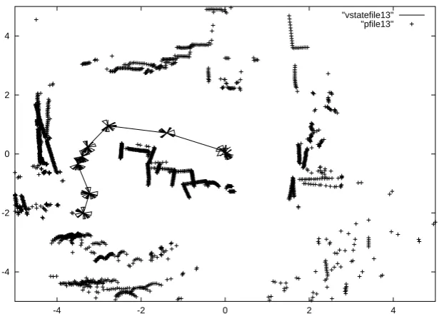
We recorded 58 trajectories, each taking between 30 and 90 seconds to complete, with the robot navigating approximately 10 metres. Our environment was unstruc-tured, consisting of a cluttered open space open to human traffic. We made the environment vary between trajectories, from sparsely to highly cluttered and very dynamic. Figure 9 shows a typical environment configuration. The space is an open area within a busy laboratory. Obstacles are placed within the space. The picture shows the positions of the obstacles and of the desks and walls bounding the area, according to the laser readings of the robot. The positions of the obstacles are plot-ted according to readings taken at different points along the trajectory. The local-isation technique being used by the robot is based on odometry which explains inaccuracies in the alignments of the obstacle positions as seen from different loca-tions. The approximate trajectory of the robot is shown as it travels from its starting point to its destination in a given run. At each of the points shown the laser scan is represented by a collection of sectors each of which represents a segment that is devoid of obstacles according to the laser scanner.

The state of the system was sampled at a frequency of 5 Hz. Each sampling recorded the values of 16 variables including the following raw features: the coordinate po-sition of the robot, relative to its starting popo-sition within a given coordinate system; the laser readings indicating the positions of obstacles and their proximity to the

robot; the speed at which the robot was travelling in the x and y directions; the

angular velocity of the robot and the Euclidean distance travelled since the last measurement.

-4 -2 0 2 4

-4 -2 0 2 4

"vstatefile13" "pfile13"

Fig. 9. A typical environment configuration from the robot’s point of view.

4.2 The navigation states

In our experiment we used an a priori set of labels consisting of two visible states (the starting and finishing states) and four subjective states (hesitation, obstacle avoidance, progress and search). The progress state is the state in which the robot is moving unencumbered through the environment. Hesitation is the state in which the robot is temporarily trapped in a highly cluttered region and is unsure how to proceed. Searching represents the robot embarking on routes, which turn out to be dead ends, in its effort to find a path. Obstacle avoidance is visually distinguishable from hesitation and searching because the robot is typically making progress and then veers to avoid something in its path. We did not identify any failure states in this experiment although it would be straightforward to include failing trajectories (when the robot collides with an obstacle it prematurely terminates its trajectory) and to identify the corresponding failure states. We make no limiting assumptions that prevent the inclusion of failure states. However, our robot very rarely collided with obstacles, thanks to the efficacy of its control software, so we did not gather data representative of failures in our experiment.

4.3 Sensory-motor Data and Features