Exact 1-Norm Support Vector Machines via
Unconstrained Convex Differentiable Minimization
Olvi L. Mangasarian∗ [email protected]
Computer Sciences Department University of Wisconsin Madison, WI 53706, USA
Editors: Kristin P. Bennett and Emilio Parrado-Hern´andez
Abstract
Support vector machines utilizing the 1-norm, typically set up as linear programs (Mangasarian, 2000; Bradley and Mangasarian, 1998), are formulated here as a completely unconstrained mini-mization of a convex differentiable piecewise-quadratic objective function in the dual space. The objective function, which has a Lipschitz continuous gradient and contains only one additional fi-nite parameter, can be minimized by a generalized Newton method and leads to an exact solution of the support vector machine problem. The approach here is based on a formulation of a very general linear program as an unconstrained minimization problem and its application to support vector machine classification problems. The present approach which generalizes both (Mangasar-ian, 2004) and (Fung and Mangasar(Mangasar-ian, 2004) is also applied to nonlinear approximation where a minimal number of nonlinear kernel functions are utilized to approximate a function from a given number of function values.
1. Introduction
One of the principal advantages of 1-norm support vector machines (SVMs) is that, unlike 2-norm SVMs, they are very effective in reducing input space features for linear kernels and in reducing the number of kernel functions (Bradley and Mangasarian, 1998; Fung and Mangasarian, 2004) for nonlinear SVMs. With few exceptions, the simplex method (Dantzig, 1963) has been the exclusive algorithm for solving norm SVMs. The interesting paper (Zhu et al., 2004) which treats the 1-norm SVM uses standard linear programming packages for solving their formulation. To the best of our knowledge there has not been an exact completely unconstrained differentiable minimiza-tion formulaminimiza-tion of 1-norm SVMs, which is the principal concern of the present rather theoretical contribution which we outline now.
In Section 2 we show how a very general linear program can be solved as the minimization of a completely unconstrained differentiable piecewise-quadratic convex function that contains a single finite parameter. This result generalizes (Mangasarian, 2004) where linear programs with millions of constraints were solved as unconstrained minimization problems by a generalized New-ton method. In Section 3 we show how to set up 1-norm SVMs, with linear and nonlinear kernels as unconstrained minimization problems and state a generalized Newton method for their solution. In Section 4 we show how to solve the problem of approximating an unknown function based on a given number of function values using a minimal number of kernel functions. We achieve this
by again converting a 1-norm approximation problem to an unconstrained minimization problem. Computational results given in Section 5 show that the proposed approach is faster than a conven-tional linear programming solver, CPLEX (ILO, 2003), and faster than another related method as well as having better input space feature suppression for a linear classifier and mostly better kernel function suppression for a nonlinear classifier. Section 6 concludes the paper.
We now describe our notation and give some background material. All vectors will be column vectors unless transposed to a row vector by a prime′. For a vector x in the n-dimensional real space Rn, x+ denotes the vector in Rn with all of its negative components set to zero. This corresponds
to projecting x onto the nonnegative orthant. For a vector x∈Rn, x∗denotes the vector in Rn with
components(x∗)i=1 if xi>0 and 0 otherwise (i.e. x∗is the result of applying the step function
component-wise to x). For x∈Rn,kxk1,kxkandkxk∞, will denote the 1−, 2−and∞−norms of x.
For simplicity we drop the 2 fromkxk2. The notation A∈Rm×nwill signify a real m×n matrix. For
such a matrix A′will denote the transpose of A, Aiwill denote the i-th row of A and Ai jwill denote the
i j-th element of A. A vector of ones or zeroes in a real space of arbitrary dimension will be denoted by e or 0, respectively. For a piecewise-quadratic function such as, f(x) =1
2||(Ax−b)+|| 2+1
2x ′Px,
where A∈Rm×n, P∈Rn×n, P=P′, P positive semidefinite and b∈Rm, the ordinary Hessian does not exist because its gradient, the n×1 vector∇f(x) =A′(Ax−b)++Px, is not differentiable but is Lipschitz continuous with a Lipschitz constant ofkA′k kAk+kPk. However, one can define its
generalized Hessian (Hiriart-Urruty et al., 1984; Facchinei, 1995; Mangasarian, 2001) which is the n×n symmetric positive semidefinite matrix:
∂2f(x) =A′diag(Ax−b) ∗A+P,
where diag(Ax−b)∗ denotes an m×m diagonal matrix with diagonal elements (Aix−bi)∗, i=
1, . . . ,m. The generalized Hessian has many of the properties of the regular Hessian (Hiriart-Urruty et al., 1984; Facchinei, 1995; Mangasarian, 2001) in relation to f(x). If the smallest eigenvalue of
∂2f(x)is greater than some positive constant for all x∈Rn, then f(x)is a strongly convex
piecewise-quadratic function on Rn. A separating plane, with respect to two given point sets
A
andB
in Rn,is a plane that attempts to separate Rn into two halfspaces such that each open halfspace contains points mostly of
A
orB
. The notation :=denotes a definition.2. Linear Programs as Exact Unconstrained Differentiable Minimization Problems
We consider in this section a very general linear program (LP) that contains nonnegative and un-restricted variables as well as inequality and equality constraints. We will show how to obtain an exact solution of this LP by a single minimization of a completely unconstrained differentiable piecewise-quadratic function that contains a single finite parameter. We begin with the primal linear program:
min
(x,y)∈Rn+ℓc
′x+d′y s.t. Ax+By≥b,Ex+Gy=h,x≥0, (1)
where c∈Rn, d∈Rℓ, A∈Rm×n, B∈Rm×ℓ, E∈Rk×n, G∈Rk×ℓ, b∈Rmand h∈Rk, and its dual:
max
(u,v)∈Rm+kb
′u+h′v s.t. A′u+E′v≤c,B′u+G′v=d,u≥0. (2)
The exterior penalty problem for the dual linear program is:
min
(u,v)∈Rm+kε(−b
′u−h′v) +1
2(k(A
′u+E′v−c)
Solving the exterior penalty problem for a positive sequence {εi} converging to zero will yield a
solution to the dual linear program (2) (Fiacco and McCormick, 1968; Bertsekas, 1999). However, we will not do that here because of the inherent inaccuracies associated with asymptotic exterior penalty methods and the fact that this would merely yield an approximate dual solution but not a primal solution. Instead, we will solve the exterior penalty problem for some finite value of the penalty parameter ε and from this inexact dual solution we shall easily extract an exact primal solution by using the following proposition.
Proposition 1 Exact Primal Solution Computation Let the primal LP (1) be solvable. Then the dual exterior penalty problem (3) is solvable for allε>0. For anyε∈(0,¯ε]for some ¯ε>0, any solution(u,v)of (3) generates an exact solution to primal LP (1) as follows:
x= 1
ε(A′u+E′v−c)+, y=
1
ε(B′u+G′v−d). (4)
In addition, this(x,y)minimizes:
kxk2+kyk2+kAx+By−bk2, (5) over the solution set of the primal LP (1).
Proof The dual exterior penalty minimization problem (3) can be written in the equivalent form:
min
(u,v,z1,z2)∈Rm+k+n+m
ε(−b′u−h′v) +1
2(kz1k
2+kB′u+G′v−dk2 + kz 2k2)
s.t. −A′u−E′v+c+z1 ≥ 0
u+z2 ≥ 0.
(6)
The justification for this is that at a minimum of (6) the variables z1and z2 are nonnegative, else
if any component of these variables is negative the objective function can be strictly decreased by setting that component to zero while maintaining constraint feasibility. Hence, at a solution of (6), z1= (A′u+E′v−c)+and z2= (−u)+. The Wolfe dual (Mangasarian, 1994, Problem 8.2.2) for the
convex quadratic program (6) is:
max
(u,v,z1,z2,r,s)∈Rm+k+n+m+n+m
−1 2((kz1k
2+kB′uk2+kG′vk2+2v′GB′u− kdk2+kz
2k2) − c′r
s.t.−εb+B(B′u+G′v−d) +Ar−s = 0 −εh+G(B′u+G′v−d) +Er = 0 z1=r ≥ 0
z2=s ≥ 0,
(7)
which can be written in the equivalent form:
− min
(u,v,r,s)∈Rm+k+n+m
1 2(krk
2+kB′uk2+kG′vk2+2v′GB′u− kdk2+ksk2) + c′r
s.t.−b+B(B′u+G′v−d
ε ) +Arε=εs ≥ 0 −h+G(B′u+Gε′v−d) +Eεr = 0
r ≥ 0.
Note that at a solution of the exterior penalty problem (6) and the corresponding Wolfe dual (7) we have that:
r=z1 = (A′u+E′v−c)+
s=z2 = (−u)+. (9)
Define now:
x := rε =1ε(A′u+E′v−c)+
y := 1
ε(B′u+G′v−d), (10)
where the equality in (10) follows from (9). Substituting (10) in (8) gives, after some algebra, the optimization problem (11) below. It is easiest to see that (8) follows from (11) if we substitute for x and y from (10) in (11) below and note that 0≤r=εx and that 0≤s=ε(Ax+By−b)which follow from the constraints of (8) and the definitions (10) of x and y.
− min
(x,y)∈Rn+ℓc
′x+d′y + ε
2(kxk2+kyk2+kAx+By−bk2)
Ax+By ≥ b
Ex+Gy = h
x ≥ 0.
(11)
This convex quadratic program (11) is feasible, because the linear program (1) is feasible. It is solvable for anyε>0 (Frank and Wolfe, 1956) because its objective function is bounded below since it is a strongly convex quadratic function in(x,y). Since the dual exterior penalty minimization problem objective (3) or equivalently (6) is bounded below by the negative of the objective function of (11) by the weak duality theorem (Mangasarian, 1994, Theorem 8.2.3), hence (3) is solvable for anyε>0. By the perturbation theory of linear programs (Mangasarian and Meyer, 1979), it follows that for ε∈(0,ε¯], for some ¯ε>0, (x,y) as defined in (10) or equivalently (4), solve the linear program (1) and additionally minimize the expression (5) over the solution set of the original linear program (1).2
A more direct, but just as laborious and rather unintuitive proof of Proposition 1 can be given by showing that the KKT necessary and sufficient optimality conditions for (11) follow from the necessary and sufficient optimality conditions of setting the gradient of the exterior penalty problem (3) equal to zero. We do not give that proof here because it does not justify how the quadratic perturbation terms of (11) arose, but it merely starts with these terms as given.
We turn now to an implementation of this result for various 1-norm SVMs.
3. 1-Norm SVMs as Unconstrained Minimization Problems
We consider first the 1-norm linear SVM binary classification problem (Mangasarian, 2000; Bradley and Mangasarian, 1998; Fung and Mangasarian, 2004):
min
(w,γ,y) νkyk1+kwk1
s.t. D(Aw−eγ) +y ≥ e
y ≥ 0,
(12)
where, with some abuse of notation by multiple representation, we let the m×n matrix A in this section represent m points in Rnto be separated to the best extent possible by a separating plane:
according to the class of each row of A as given by the m×m diagonal matrix D with elements Dii=±1. The objective termkyk1 minimizes the classification error weighted with the positive
parameterνwhile the termkwk1maximizes the∞-norm margin (Mangasarian, 1999) between the
bounding planes x′w=γ±1 that approximately bound each of the two classes of points represented by A. It is well known (Bradley and Mangasarian, 1998; Fung and Mangasarian, 2004) that using kwk1 in the objective function of (12) instead of the standard 2-norm squared termkwk2(Vapnik,
2000; Sch¨olkopf and Smola, 2002) results in input space feature selection by suppressing many components of w, whereas the standard 2-norm SVM does not suppress any components of w in general. We convert (12) to an explicit linear program as in (Fung and Mangasarian, 2004) by setting:
w=p−q, p≥0,q≥0, (14)
which results in the linear program:
min
(p,q,γ,y) νe
′y+e′(p+q)
s.t. D(A(p−q)−eγ) +y ≥ e p,q,y ≥ 0.
(15)
We note immediately that this linear program is solvable because it is feasible and its objective function is bounded below by zero. Hence, Proposition 1 can be utilized to yield the following unconstrained reformulation of the problem.
Proposition 2 Exact 1-Norm SVM Solution via Unconstrained Minimization The unconstrained dual exterior penalty problem for the 1-norm SVM (15):
min
u∈Rm −εe ′u+1
2(k(A
′Du−e)
+k2+k(−A′Du−e)+k2+ (−e′Du)2+k(u−νe)+k2+k(−u)+k2),
(16) is solvable for allε>0. For anyε∈(0,ε¯]for some ¯ε>0, any solution u of (16) generates an exact solution of the 1-norm SVM classification problem (12) as follows:
w=p−q= = 1ε((A′Du−e)+−(−A′Du−e)+),
γ = −1
εe′Du,
y = 1ε(u−νe)+.
(17)
In addition this(w,γ,y)minimizes:
kwk2+γ2+kyk2+kD(Aw−eγ) +y−ek2, (18) over the solution set of the 1-norm SVM classification problem (12).
We note here the similarity between our unconstrained penalty minimization problem (16) and the corresponding problem of (Fung and Mangasarian, 2004, Equation 23). But, we also note a major difference. In the latter, a penalty parameterαmultiplies the termk(−u)+k2of equation (16) above
Mangasarian, 2004, Equation 11). However the generalized Newton method prescribed in (Fung and Mangasarian, 2004) for a sequence{α↑∞}, is applicable here withα=1. For completeness we state that result here. To do that we let f(u)denote the exterior penalty function (16). Then the gradient and generalized Hessian as defined in the Introduction are given as follows.
∇f(u) = −εe+DA(A′Du−e)+−DA(−A′Du−e)+
+Dee′Du+ (u−νe)+−(−u)+. (19)
∂2f(u) = DA(diag((A′Du−e)
∗+ (−A′Du−e)∗)A′D +Dee′D+diag((u−νe)∗+ (−u)∗) = DA(diag(|A′Du| −e)∗)A′D
+Dee′D+diag((u−νe)∗+ (−u)∗),
(20)
where the last equality follows from the equality:
(a−1)∗+ (−a−1)∗= (|a| −1)∗. (21)
To handle a nonlinear symmetric kernel K(A,B) that maps Rm×n×Rn×ℓ into Rm×ℓ and which generates, instead of the separating plane (13), the nonlinear separating surface:
K(x′,A′)Dv=γ, (22)
all we need to do is essentially to make the replacement:
A −→ K(A,A′)D, (23)
which we justify now. For a linear kernel K(A,A′) =AA′, we have that w=A′Dv, where v is a dual variable (Mangasarian, 2000) and the primal linear programming SVM (15) becomes upon using w=p−q=A′Dv and minimizing the 1-norm of v in the objective instead that of w:
min
(v,γ,y) νe
′y+kvk 1
s.t. D(AA′Dv−eγ) +y ≥ e
y ≥ 0.
(24)
Setting:
v=r−s, r≥0,s≥0, (25)
the linear program (24) becomes:
min
(r,s,γ,y) νe
′y+e′(r+s)
s.t. D(AA′D(r−s)−eγ) +y ≥ e r,s,y ≥ 0,
(26)
which is the linear kernel SVM in terms of the dual variable v=r−s. If we replace the linear kernel AA′in (26) by the nonlinear kernel K(A,A′)we obtain the nonlinear kernel linear program:
min
(r,s,γ,y) νe
′y+e′(r+s)
s.t. D(K(A,A′)D(r−s)−eγ) +y ≥ e r,s,y ≥ 0.
We immediately note that the linear program (15) is identical to the linear program (27) if we make the replacement (23).
Finally, a word regarding the choice of ε in Propositions 1 and 2. Computationally in (Fung and Mangasarian, 2004) this does not seem to be critical and is effectively addressed as follows. By (Lucidi, 1987, Corollary 3.2), if for two successive values ofε:ε1>ε2, the corresponding solutions
of theε-perturbed quadratic programs (11) are equal, then under certain assumptions these equal successive solutions constitute a solution of the linear programs (1) or (12) that also minimize the quadratic perturbations (5) or (18). This result can be implemented computationally by using anε, which when decreased by some factor yields the same solution to (1) or (12). In our computational results this turned out to either 4×10⁻⁴or 10−6.
We state now our generalized Newton algorithm for solving the unconstrained minimization problem (16) as follows.
Algorithm 3 Generalized Newton Algorithm for (16) Let f(u), ∇f(u) and∂2f(u) be defined by (16),(19) and (20). Set the parameter values ν, ε, δ, tolerance tol, and imax (typically: ε∈
[10−6,4×10⁻⁴]for linear SVMs andε∈[10−9,1]nonlinear SVMs, tol=10−3, imax=50, while
νandδare set by a tuning procedure). Start with any u0∈Rm. For i=0,1, . . .: (I) ui+1=ui−λi(∂2f(ui) +δI)−1∇f(ui) =ui+λidi,
where the Armijo stepsizeλi=max{1,12,14, . . .}is such that:
f(ui)−f(ui+λidi)≥ −
λi
4∇f(u
i)′di, (28)
and diis the modified Newton direction:
di=−(∂2f(ui) +δI)−1∇f(ui). (29) In other words, start withλi=1 and keep multiplyingλiby 12 until (28) is satisfied.
(II) Stop ifkui−ui+1k ≤tol or i=imax. Else, set i=i+1 and go to(I).
(III) Define the solution of the 1-norm SVM (12) with least quadratic perturbation (18) by (17) with u=ui.
We state a convergence result for this algorithm now.
Proposition 4 Let tol=0, imax=∞and letε>0 be sufficiently small. Each accumulation point ¯
u of the sequence {ui} generated by Algorithm 3 solves the exterior penalty problem (16). The corresponding(w¯,γ¯,y¯)obtained by setting u to ¯u in (17) is an exact solution to the primal 1-norm SVM (12) which in addition minimizes the quadratic perturbation (18) over the solution set of (12).
Proof That each accumulation point ¯u of the sequence{ui}solves the minimization problem (13) follows from exterior penalty results (Fiacco and McCormick, 1968; Bertsekas, 1999) and standard unconstrained descent methods such as (Mangasarian, 1995, Theorem 2.1, Examples 2.1(i), 2.2(iv)) and the facts that the direction choice di of (24) satisfies, for some c>0:
−∇f(ui)′di = ∇f(ui)′(δI+∂2f(ui))−1∇f(ui)
≥ ck∇f(ui)k2, (30)
and that we are using an Armijo stepsize (28). The last statement of the theorem follows from Proposition 2.2
4. Minimal Kernel Function Approximation as Unconstrained Minimization Problems
We consider here the problem of constructing a kernel function approximation from a given number of function values using the 1-norm to minimize both the error in the approximation as well as the weights of the kernel functions. Utilizing the 1-norm in minimizing the kernel weights suppresses unnecessary kernel functions similar to the approach of (Mangasarian et al., 2004) except that we shall solve the resulting linear program here through an unconstrained minimization reformulation. Also, for simplicity we shall not incorporate prior knowledge as was done in (Mangasarian et al., 2004).
We consider m given function values b∈Rm associated with m n-dimensional vectors repre-sented by the m rows of the m×n matrix A. We shall fit the data points by a linear combination of symmetric kernel functions as follows:
K(A,A′)v+eγ≈b, (31)
where the unknown parameters v∈Rmandγ∈R are determined by minimizing the 1-norm of the approximation error weighted byν>0 and the 1-norm of v as follows:
min
(v,γ)∈Rn+1νkK(A,A
′)v+eγ−bk
1+kvk1. (32)
Setting
v = r−s,r≥0,s≥0,
K(A,A′)v+eγ−b = y−z,y≥0,z≥0, (33)
we obtain the following linear program:
min
(r,s,γ,y,z) νe
′(y+z) +e′(r+s)
s.t. K(A,A′)(r−s) +eγ−y+z = b r,s,y,z ≥ 0,
(34)
which is similar to the nonlinear kernel SVM classifier linear programming formulation (27) with equality constraints replacing inequality constraints. We also note that this linear program is solv-able because it is feasible and its objective function is bounded below by zero. Hence, Proposition 1 can be utilized to yield the following unconstrained reformulation of the problem.
Proposition 5 Exact 1-Norm Nonlinear SVM Approximation via Unconstrained Minimiza-tion The unconstrained dual exterior penalty problem for the 1-norm SVM approximaMinimiza-tion (34):
min
u∈Rm −εb ′u+1
2(k(K(A,A
′)u−e)
+k2+k(−K(A,A′)u−e)+k2+ (e′u)2+k(−u−νe)
+k2+k(u−νe)+k2),
(35)
is solvable for allε>0. For anyε∈(0,ε¯]for some ¯ε>0, any solution u of (35) generates an exact of the 1-norm SVM approximation problem (32) as follows:
v=r−s= = 1ε((K(A,A′)u−e)+−(−K(A,A′)u−e)+),
γ = 1
εe′u,
y = 1ε(−u−νe)+,
z = 1
ε(u−νe)+
In addition this(r,s,γ,y,z)minimizes:
krk2+ksk2+γ2+kyk2+kzk2, (37)
over the solution set of the 1-norm SVM classification problem (34).
Computational results utilizing the linear programming formulation (32) with prior knowledge in (Mangasarian et al., 2004) but using the simplex method of solution is effective for solving ap-proximation problems. The unconstrained minimization formulation (35) is another method of solu-tion which can also handle such problems without prior knowledge as well as with prior knowledge with appropriate but straightforward modifications.
We turn now to our computational results.
5. Computational Results
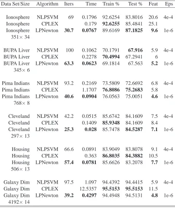
Computational testing was carried on a 3 Ghz Pentium 4 machine with 2GB of memory running CentOS 4 Linux and utilizing the CPLEX 7.1 (ILO, 2003) linear programming package within MATLAB 7.1 (MATLAB, 1994-2001). We tested our algorithm on six publicly available data sets. Five from the UCI Machine Learning Repository Murphy and Aha (1992): Ionosphere, Cleveland Heart, Pima Indians, BUPA Liver and Housing. The sixth data set, Galaxy Dim, is available from Odewahn et al. (1992). The results are summarized in Tables 1 and 2.
For the linear classifier (13) we compare in Table 1, NLPSVM (Fung and Mangasarian, 2004), CPLEX (ILO, 2003) and our Generalized LPNewton Algorithm for (16), on six public data sets using ten-fold cross validation. NLPSVM is essentially identical to our algorithm, except that it requires a penalty parameter multiplying the last term of (16) to approach infinity. CPLEX uses the standard linear programming package CPLEX (ILO, 2003) to solve (26). We note that our method LPNewton is faster than both NLPSVM and CPLEX on all six data sets and gives the best feature suppression based on the average number of features used by the linear classifier (13). NLPSVM has the best test set correctness on two of the data sets, and comparable correctness on the other four. The Armijo step size was not needed in either NLPSVM or LPNewton. Tuning on 10% of the training set was used to determine the parametersνandδfrom the sets{2−12, . . . ,212}and
{10−3, . . . , .103}respectively. Epsilon was set to the value 4.00E-04 used in (Fung and Mangasarian,
2004) for NLPSM and to 1.00E-06 for our LPNewton algorithm.
Data Set/Size Algorithm Iters Time Train % Test % Feat Eps
Ionosphere NLPSVM 69 0.1796 92.6254 83.8016 20.6 4e-4
Ionosphere CPLEX 0.179 92.6255 85.4841 25.1
Ionosphere LPNewton 30.7 0.0767 89.6169 87.1825 9.6 1e-6
351×34
BUPA Liver NLPSVM 100 0.1062 70.1791 67.916 5.9 4e-4
BUPA Liver CPLEX 0.2278 70.4994 67.2941 6
BUPA Liver LPNewton 63.3 0.0623 69.1814 67.563 5.2 1e-6
345×6
Pima Indians NLPSVM 93.2 0.2169 73.5809 72.6692 6.8 4e-4
Pima Indians CPLEX 1.1707 76.8086 75.2683 5.8
Pima Indians LPNewton 40.6 0.0904 76.0563 75.0051 4.6 1e-6
768×8
Cleveland NLPSVM 42.2 0.0515 85.6742 84.1609 7.5 4e-4
Cleveland CPLEX 0.1409 85.9348 84.1609 8.4
Cleveland LPNewton 25.3 0.028 85.7478 84.5287 7.1 1e-6
297×13
Housing NLPSVM 66.6 0.0891 83.9049 83.8078 9.1 4e-4
Housing CPLEX 0.363 86.8035 84.3882 10.5
Housing LPNewton 57.4 0.0781 85.6626 83.2078 7.7 1e-6
506×13
Galaxy Dim NLPSVM 97.5 1.097 94.4392 94.4415 5.9 4e-4
Galaxy Dim CPLEX 12.5357 95.5153 95.5153 11.5
Galaxy Dim LPNewton 39.2 0.4297 94.4948 94.5131 4.8 1e-6
4192×14
Table 1: Comparison of the Linear Classifier (13) obtained by NLPSVM (Fung and
Data Set/Size Algorithm Iters Time Train % Test % Card(v) Eps
Ionosphere NLPSVM 81.7 0.181 92.0242 89.4683 18.5 4e-4
Ionosphere CPLEX 0.1555 94.7773 91.4683 15.5
Ionosphere LPNewton 36.5 0.103 92.5297 91.1587 11.2 1e-6
351×34
BUPA NLPSVM 88.3 0.1706 68.8514 65.2521 15.5 4e-4
BUPA CPLEX 0.2552 74.1061 69.2521 17.3
BUPA LPNewton 88.2 0.1345 73.6572 70.6975 25.5 1e+0
345×6
Cleveland NLPSVM 84.6 0.1128 83.168 80.4368 9.1 4e-4
Cleveland CPLEX 0.1097 85.0383 81.8161 11.8
Cleveland LPNewton 80.2 0.1061 83.0151 82.8621 5.6 1e-9
297×13
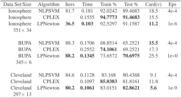
Table 2: Comparison of the Nonlinear Classifier (22) obtained by NLPSVM (Fung and
6. Conclusion and Outlook
We have derived an unconstrained differentiable convex minimization reformulation of a most gen-eral linear program and have applied it to 1-norm classification and approximation problems. Very effective computational results of our method on special cases of general linear programs (Man-gasarian, 2004) and an approximate version for support vector machine classification (Fung and Mangasarian, 2004), as well as computational results presented in Section 5, lead us to believe that the proposed unconstrained reformulation of very general linear programs and support vector ma-chines is a very promising computational method for solving such problems as well as extensions to knowledge-based formulations (Mangasarian, 2005; Fung et al., 2003; Mangasarian et al., 2004).
Acknowledgments
I am indebted to my PhD student Michael Thompson for the computational results given in this work. Research described in this Data Mining Institute Report 05-03, August 2005, was supported by National Science Foundation Grants CCR-0138308 and IIS-0511905, the Microsoft Corporation and ExxonMobil. Revised January 2006.
References
D. P. Bertsekas. Nonlinear Programming. Athena Scientific, Belmont, MA, second edition, 1999.
P. S. Bradley and O. L. Mangasarian. Feature selection via concave minimization and support vector machines. In J. Shavlik, editor, Machine Learning Proceedings of the Fifteenth Interna-tional Conference(ICML ’98), pages 82–90, San Francisco, California, 1998. Morgan Kaufmann. ftp://ftp.cs.wisc.edu/math-prog/tech-reports/98-03.ps.
G. B. Dantzig. Linear Programming and Extensions. Princeton University Press, Princeton, New Jersey, 1963.
F. Facchinei. Minimization of SC1functions and the Maratos effect. Operations Research Letters, 17:131–137, 1995.
A. V. Fiacco and G. P. McCormick. Nonlinear Programming: Sequential Unconstrained Minimiza-tion Techniques. John Wiley & Sons, New York, NY, 1968.
M. Frank and P. Wolfe. An algorithm for quadratic programming. Naval Research Logistics Quar-terly, 3:95–110, 1956.
G. Fung and O. L. Mangasarian. A feature selection Newton method for support vector
ma-chine classification. Computational Optimization and Applications, 28(2):185–202, July 2004. ftp://ftp.cs.wisc.edu/pub/dmi/tech-reports/02-03.ps.
J.-B. Hiriart-Urruty, J. J. Strodiot, and V. H. Nguyen. Generalized hessian matrix and second-order optimality conditions for problems with CL1 data. Applied Mathematics and Optimization, 11: 43–56, 1984.
ILOG CPLEX 9.0 User’s Manual. ILOG, Incline Village, Nevada, 2003.
http://www.ilog.com/products/cplex/.
Y.-J. Lee and O. L. Mangasarian. RSVM: Reduced support vector machines. In Proceedings of the First SIAM International Conference on Data Mining, Chicago, April 5-7, 2001, CD-ROM, 2001. ftp://ftp.cs.wisc.edu/pub/dmi/tech-reports/00-07.ps.
S. Lucidi. A new result in the theory and computation of the least-norm solution of a linear program. Journal of Optimization Theory and Applications, 55:103–117, 1987.
O. L. Mangasarian. Nonlinear Programming. SIAM, Philadelphia, PA, 1994.
O. L. Mangasarian. Parallel gradient distribution in unconstrained optimization. SIAM
Journal on Control and Optimization, 33(6):1916–1925, 1995. ftp://ftp.cs.wisc.edu/tech-reports/reports/1993/tr1145.ps.
O. L. Mangasarian. A finite Newton method for classification problems. Technical Report 01-11, Data Mining Institute, Computer Sciences Department, University of Wisconsin, Madison, Wis-consin, December 2001. ftp://ftp.cs.wisc.edu/pub/dmi/tech-reports/01-11.ps.Optimization Meth-ods and Software 17, 2002, 913-929.
O. L. Mangasarian. A Newton method for linear programming. Journal of Optimization Theory and Applications, 121:1–18, 2004. ftp://ftp.cs.wisc.edu/pub/dmi/tech-reports/02-02.ps.
O. L. Mangasarian. Knowledge-based linear programming. SIAM Journal on Optimization, 15: 375–382, 2005. ftp://ftp.cs.wisc.edu/pub/dmi/tech-reports/03-04.ps.
O. L. Mangasarian. Arbitrary-norm separating plane. Operations Research Letters, 24:15–23, 1999. ftp://ftp.cs.wisc.edu/math-prog/tech-reports/97-07r.ps.
O. L. Mangasarian. Generalized support vector machines. In A. Smola, P. Bartlett, B. Sch¨olkopf, and D. Schuurmans, editors, Advances in Large Margin Classifiers, pages 135–146, Cambridge, MA, 2000. MIT Press. ftp://ftp.cs.wisc.edu/math-prog/tech-reports/98-14.ps.
O. L. Mangasarian and R. R. Meyer. Nonlinear perturbation of linear programs. SIAM Journal on Control and Optimization, 17(6):745–752, November 1979.
O. L. Mangasarian, J. W. Shavlik, and E. W. Wild. Knowledge-based kernel approximation.
Journal of Machine Learning Research, 5:1127–1141, 2004. ftp://ftp.cs.wisc.edu/pub/dmi/tech-reports/03-05.ps.
MATLAB. User’s Guide. The MathWorks, Inc., Natick, MA 01760, 1994-2001.
http://www.mathworks.com.
P. M. Murphy and D. W. Aha. UCI machine learning repository, 1992.
S. Odewahn, E. Stockwell, R. Pennington, R. Humphreys, and W. Zumach. Automated star/galaxy discrimination with neural networks. Astronomical Journal, 103(1):318–331, 1992.
B. Sch¨olkopf and A. Smola. Learning with Kernels. MIT Press, Cambridge, MA, 2002.
V. N. Vapnik. The Nature of Statistical Learning Theory. Springer, New York, second edition, 2000.