Absent Data Generating Classifier for Imbalanced Class Sizes

Absent Data Generating Classifier for Imbalanced Class Sizes

Arash Pourhabib [email protected]

School of Industrial Engineering and Management Oklahoma State University

322 Engineering North, Stillwater, Oklahoma 74078-5016, USA

Bani K. Mallick [email protected]

Department of Statistics Texas A&M University

3143 TAMU, College Station, TX 77843-3143, USA

Yu Ding [email protected]

Department of Industrial and Systems Engineering Texas A&M University

3131 TAMU, College Station, TX 77843-3131, USA

Editor:Russ Greiner

Abstract

We propose an algorithm for two-class classification problems when the training data are imbalanced. This means the number of training instances in one of the classes is so low that the conventional classification algorithms become ineffective in detecting the minority class. We present a modification of the kernel Fisher discriminant analysis such that the imbalanced nature of the problem is explicitly addressed in the new algorithm formulation. The new algorithm exploits the properties of the existing minority points to learn the effects of other minority data points, had they actually existed. The algorithm proceeds iteratively by employing the learned properties and conditional sampling in such a way that it generates sufficient artificial data points for the minority set, thus enhancing the detection probability of the minority class. Implementing the proposed method on a number of simulated and real data sets, we show that our proposed method performs competitively compared to a set of alternative state-of-the-art imbalanced classification algorithms.

Keywords: kernel Fisher discriminant analysis, imbalanced data, two-class classification

1. Introduction

Classification is a task of supervised learning in which the response function assumes a set of integer values known as the class labels. In particular, two-class classification refers to algorithms producing binary responses and aiming at separating two probability densities after observing some instances from each class. In this paper, we are interested in developing a classification algorithm for a two-class classification problem in which the number of data points in one class (i.e. the majority class) is greater than those of the other class (i.e. the minority class). This type of data structure is called imbalanced data.

the minority class is the class of defective products; in security applications, the minority class is the class of potential perpetrators or attackers; in medical applications, the minority class is the class of diseases or cancerous cells. A classification method that fails to detect the minority classes is useless for practical purposes.

If one is interested in detecting minority cases in application, a direct use of traditional two-class classifications, such as support-vector machines or logistic regression, is not reliable because when the minority class data are too few in the training set, those methods tend to label almost all the instances in the test set, minority or otherwise, as the majority class (Chen et al., 2005). A training data set overwhelmed with one class of data points and deficient in the other class misleads the two classification algorithms about the accurate boundary between the two groups. Using most standard loss functions, these classification algorithms see little penalty by classifying regions in which both the minority and majority points have high density.

The major efforts aimed at solving the imbalanced classification problem can be cate-gorized into: (a) cost-sensitive methods and (b) sampling strategies (He and Garcia, 2009; Japkowicz, 2000). Cost-sensitive methods take the imbalance structure into account by assigning a higher cost to the miss-classification of minority data points (Elkan, 2001; Ting, 2002). Despite a theoretical connection between imbalanced structure and cost-sensitive framework (Maloof, 2003; Weiss, 2004), this class of algorithms however may fail in prac-tice; for example, if in the training stage the instances forming the classes are separable (Wallace et al., 2011, p.757). More critically, determining a suitable cost function is not a straightforward task and it may be difficult to achieve a robust algorithm using cost-sensitive methods.

The basic idea of the sampling-based approach is to alter the imbalanced structure of the problem by using different types of sampling methods. Hence, the algorithms in this category can be classified according to the specific sampling approaches, including resampling with replication, undersampling, or synthetic oversampling. In resampling with replication, one can use, for instance, bootstrapping for oversampling the minority data (Chen et al., 2005; Byon et al., 2010). In undersampling, one downsamples the majority data points to create more balanced data sets and alleviate the imbalance attached to the original data (Liu et al., 2009).

A novel approach proposed by Chawla et al. (2002) and called SMOTE, generates extra synthetic minority data points by interpolating the spaces between existing minority data points. Unlike other sampling methods which resample the existing data, SMOTE “creates” new data points, debuting the synthetic oversampling approach. Since SMOTE, many other variations of synthetic oversampling have been proposed in the literature; among others, Han et al. (2005) proposed an algorithm generating minority data points close to the boundary of the two classes and Batista et al. (2004) utilized different heuristics to integrate with synthetic oversampling.

the inductive inference (Akbani et al., 2004). In other words, generating extra synthetic minority data points resembles that of using test sets in learning (Gammerman et al., 1998). SMOTE, for instance, does not employ a sophisticated approach for data synthesizing, but uses a simple, yet proved highly effective in practice, data interpolation (Chawla et al., 2002). It is not clear, however, whether the mechanism of data synthesizing matters and if so, which type of mechanism to use.

The current literature does not seem to present a consensus concerning the effectiveness of data synthesizing mechanisms. We tend to believe that it matters, because if a data synthesizing mechanism is tailored to and/or embedded in a specific classification problem, we expect to observe improvements in classification performance. Some empirical evidence supports our belief (Han et al., 2005). At a minimum, we believe that the data synthesizing issue remains unsettled and is worth further investigation.

We also believe that an important question to ponder is how to decide the decision boundary if we were furnished with more instances of the minority class. It should be emphasized, however, that not all those could-be minority points carry the same amount of information; those that can guide the algorithm to expand the minority class’s region are more valuable because it is the difficulty that classification algorithms confront. Basically the question becomes how to use the current data points to synthesize the “valuable” but absent minority data points that allow us to obtain a tighter boundary for the majority class.

Towards that goal, we employ the kernel trick embedded in Fisher discriminant analysis (Hofmann et al., 2008; Mika et al., 1999) in our data synthesizing mechanism in order to exploit the properties of newly generated points in the feature space without actually specifying them. We utilize two properties of the “artificially” generated minorities: (i) the points should be located as close as possible to the boundary of the majority class, (ii) their projection onto a lower dimensional space should be close to that of the existing minority points in their vicinity. Then we sample more minority points from the augmented data set, conditional on the boundary achieved. We perform this procedure iteratively until the algorithm achieves the desired performance, and label the resulting algorithm Absent Data Generator (ADG).

The remainder of this paper is organized as follows. Section 2 outlines the kernel Fisher discriminant analysis, formally defines the imbalanced classification problem and presents the main optimization formulation. Section 3 presents the details of the proposed algorithm. Section 4 describes the proposed method’s application to several simulated and real data sets and the results when the data structure is imbalanced. Section 5 discusses finding a bound on the generalization error of the algorithm. Section 6 concludes the paper and offers suggestions for future research.

2. Problem Formulation

LetX denote the input space, and supposeX−={x−₁,x−₂, . . . ,x−_l−} ⊂ X is the training set of majority data points which are independent and identically distributed (i.i.d.) (negative points, labeled as −1 or simply “−”) andX+ _={x+

1,x+2, . . . ,x+l+} ⊂ X is the training set

case of imbalance data, we have l+ l−, or simply l l−. The goal in this section is to introduce a basic framework and general thoughts on how to generate and then utilize artificial data points. We propose generating artificial data points near the discriminative boundary of the two classes, and that they are generated within existing clusters with the probability of artificial data generated within a cluster inversely proportional to the size of that cluster.

First, we introduce the notion of “absent data”: intuitively, absent data refer to the data points belonging to the minority class whose lack of presence has made the problem imbalanced, and we intend to re-generate them for the purpose of two-class classification. The concept of some data being absent is based on the thought that the existing data points may convey some information that allows us to identify some new data points belonging to the same class. Of course, acknowledging the existing of absent data does not imply that we know their numbers or exact locations in the spacea priori. But in the context of imbalanced classification, this assumption paves the way for solving the problem through synthetic oversampling of minority data. LetZ ={x+_l+1,x+_l+2, . . . ,x+_l+k} ⊂ X+_{denote these} absent data from the minority class; we assume the absent data are also an i.i.d. sample. We may denote eachx+_l+j ∈ Z by zj for j= 1,2, . . . , k.

We first review the Fisher discriminant analysis briefly. For a two-class classification, Fisher linear discriminant can be expressed simply through the following optimization prob-lem:

max

w J(w) =

wTSBw

wT_S Ww

, (1)

whereSB and SW are the between and within class scatter matrices, respectively:

SB= (m−−m+)(m−−m+)T,

SW =

X

i∈{−,+}

X

x∈Xi

(x−mi)(x−mi)T, (2)

and mi = _l1_i

Pli

j=1xij, for i ∈ {−,+}, is the sample average of each class. Problem (1) can be interpreted as maximizing the ratio of the between-class variance to the pooled variance about the means. Under certain conditions, we can also interpret this formulation as an optimal Bayes classifier (Bickel and Levina, 2004). We will revisit this formulation in Section 5 when developing an error bound.

To deal with nonlinear cases, one can map the data into a high-dimensional feature space and perform the calculation in that space. However, if an appropriate kernel is chosen for the transformation of the data and the calculation only requires kernel evaluations, we do not have to perform any calculations in the high-dimensional feature space (Hofmann et al., 2008). This property, known as the kernel trick, can be applied to the Fisher discriminant analysis, resulting in the Kernel Fisher Discriminant (KFD) (Mika et al., 1999). Specifically, the KFD is the extension of the Fisher linear discriminant performed in the feature space which solves

max

w J(w) =

wTSφ_Bw

wT_Sφ Ww

where Sφ_B and Sφ_W are the between and within class scatter matrices, respectively, in the feature space:

Sφ_B= (mφ₋−mφ₊)(mφ₋−mφ₊)T,

Sφ_W = X i∈{−,+}

X

x∈Xi

(φ(x)−mφ_i )(φ(x)−mφ_i )T, (4)

and mφ_i = _l1

i

Pli

j=1φ(xij). Here, φis a nonlinear mapping fromX to the feature space F, which is assumed to be a separable Hilbert space endowed with an inner producth·,·i such that there exists a functionK :X × X →_RwhereK(x,x0) =hφ(x),φ(x0)i. Obviously, in this casew∈ F . Applying to imbalanced data sets, KFD suffers the same problem as most other classifiers do, i.e. it falls short of detecting most minority points in the test stage.

Our goal is to consider the imbalanced structure explicitly and extend KFD in such a way that it could be applied to imbalanced data. Towards this end, our thought process is as follows: first, if we had extra data points from the minority class, those points would be projected with high probability to where the existing minority points are projected; second, points close to the boundary of the majority points carry more “information” so we can use them to find the separating hyperplane in the feature space. The latter is in fact an intuitive property we are seeking, but the former requires more clarification. Particularly, if dealing with complex patterns in high dimensions, we may frequently observe that the minority data points constitute separate clusters after (or before) being projected to a lower-dimensional space. Therefore, if resemblance in projection regions is used as a property to generate artificial data, it entails precaution against the effect of complex structures. One way to address this issue is to take the cluster-based structure of the data into account explicitly.

Suppose the training minority points constitute C different clusters, for C ≥ 1. That is, we have X+₌SC

c=1Xc+ and Xc+0 ∩ X_c+ =∅forc6=c0, whereX_c+={x+_1,c,x+_2,c,· · ·,x+_l

c,c}

is the c-th cluster of the minority data points, and we have |X+

c | = lc, and PCc=1lc = l. Accordingly, we partition the absent data in Z also into C different clusters, Zc’s, for c= 1,2, . . . , C, each of which corresponds to one of the C clusters of the minority points. Specifically Z_c={x+_l

c+1,c,x

+

lc+2,c, . . . ,x

+ lc+kc,c},

SC

c=1Zc=Z, andZc0 ∩ Z_c=∅, forc6=c0. We also have |Zc| = kc, and PC_c=1kc = k. The previously defined notation zj can be similarly extended as zj,c :=x+_lc+j,c, forj= 1,2,· · · , kc.

To enforce the property that newly generated points would be projected with high probability to where the existing minority points are projected, we add the constraint

wTφ(zj,c)−wTmφ_+,c 2

≤δ, for j= 1,2, . . . kc, c= 1,2, . . . C, (5)

for some positiveδ >0, wheremφ_+,c= _l1

c

Plc

j=1φ(x+j,c), namely the mean of cluster cin the feature space. To have the second property, i.e. to have more points close to the boundary of the majority points, we add another constraint,

(φ(zj,c)−mφ−)T(φ(zj,c)−mφ−)≤Λ for j= 1,2, . . . kc, c= 1,2, . . . C, (6)

only one cluster is determined according to the algorithm discussed in Section 3, which means that the constraint implies that the newly generated data point is at mostδ distance away from the mean of the minority data points. Constraint (6) ensures that the newly generated points are “useful” in the sense that they are located close to the boundary of the two groups.

As a result of the Representer’s Theorem (Hofmann et al., 2008), we can safely assume bothwandφ(zj,c) belong to the space generated by the training points, namelyX−∪ X+, whose elements, with a slight abuse of notation, can be represented by {xp}np=1 where n=l−+l. Specifically,

w= n

X

p=1

αpφ(xp), (7)

and

φ(zj,c)−mφ−= n

X

p=1

β_pj,cφ(xp), for j = 1,2, . . . kc, c= 1,2, . . . C, (8)

whereαp and βpj,c are real coefficients forp= 1,2, . . . , n,j= 1,2, . . . , kcand c= 1,2, . . . C. Having made these assumptions, we can express constraints (5) and (6) as





n

X

p=1

αpφ(xp)T





n

X

p=1

βj,c_p φ(xp) + 1 l−

l−

X

`=1

φ(x−_`)− 1 lc

lc

X

`=1

φ(x+_` )



 



2

≤δ, (9)

and

n

X

p=1

(βj,c_p )2K(xp,xp)≤Λ, for j = 1,2, . . . kc, c= 1,2, . . . C, (10) respectively. In the matrix forms, the above two expressions can be represented as

αTKβj,c+αT(M−−Mc+)

2

≤δ, for j= 1,2, . . . kc, c= 1,2, . . . C, (11)

and

(βj,c)TK(βj,c)≤Λ, for j = 1,2, . . . kc, c= 1,2, . . . C, (12)

where α = [α1, α2, . . . , αn]T and βj,c = [β₁j,c, β₂j,c, . . . βnj,c]T, and M− is an n×1 vector such that (M−)j = _l−1 Pl−

`=1K(xj,x −

` ), and M c

+ is an n×1 vector such that (Mc+)j = 1

lc

Plc

`=1K(xj,x+<sub>`,c</sub>). Then×nmatrixK consists of all of the pairwise kernel evaluations, namely (K)_r,s=K(xr,xs), forr, s∈ {1,2, . . . , n}.

Following the notation introduced in Mika et al. (1999),

M := (M−−M+)(M−−M+)T, and (13)

N := X

i∈{−,+}

Ki(I−1li)K

T

i, (14)

identity matrix of appropriate size, and1li is a matrix of appropriate size whose entries are

1

li fori=−andi= +, respectively. Now, we can formulate the classification problem with

imbalanced data through the following optimization

max

α J(α) =

αTM α

αT_{N α}, (15)

subject to

αTKβj,c+αT(M−−Mc+)

2

≤δ, for j= 1,2, . . . kc, c= 1,2, . . . C, (16)

(βj,c)TK(βj,c)≤Λ, for j= 1,2, . . . kc, c= 1,2, . . . C. (17)

To solve optimization problem (15)-(17), we assume δ = 0. This implies that the newly generated points zj,c should be projected where the mean of the corresponding cluster in the minority group is projected. As such, constraint (16) is replaced by

αTKβj,c+αT(M−−M+) = 0, for j= 1,2, . . . kc, c= 1,2, . . . C.

This new constraint is not restricting, since we next solve a relaxation of the original prob-lem. Specifically, we use the Lagrangian relaxation (Anstreicher and Wolkowicz, 1998) for solving (17). First, note that an equivalent way of writing the optimization ((15))-(17) is to consider the denominator in the objective function (15) as another constraint and only have the numerator in the objective function. Specifically, we consider the objective function to be

max

α J(α) =α

T_{M α, (18)}

and add the constraint

αTN α≤R, (19)

to the optimization problem (15), for some positive number R. Having done that, we get the following for the Lagrangian function

J(α,β) =αTM α − γ

αTN α−R

− C

X

c=1 kc

X

j=1 λc_j

αTKβj,c+αT(M−−Mc₊)

− C

X

c=1 kc

X

j=1 µc_j

(βj,c)TK(βj,c)−Λ

, (20)

forγ, λc_j, µc_j >0.

To find the stationary points, we set the partial derivatives of the Lagrangian to zero,

∂

∂αJ = 2 (M −γN)α−

C

X

c=1 kc

X

j=1

∂

∂βj,cJ =−λ

c

j(Kα)−2µcjKβj,c = 0, for j= 1,2, . . . kc, c= 1,2, . . . C. (22)

Substituting βj,c =−λ

c j

2µc

jα, which results from (22), into (21) yields

2 (M−γN)α=− C X c=1 kc X j=1

λc_j K λ

c j 2µc

j

α+ (M−−Mc+)

!

, (23)

which can be further simplified as

(M−γN)α=−Kα

C X c=1 kc X j=1 (λc_j)2

4µc_j − C X c=1   

(M−−Mc₊) kc

X

j=1 λc_j

2

 



. (24)

Letω =−PC

c=1

Pkc

j=1 (λc

j)2

4µc

j , andν

c₌₋Pkc

j=1 λc

j

2 . Then, we have

(M −γN)α=Kαω+ C

X

c=1

(M−−Mc+)νc . (25)

Therefore, α is the solution of the linear system

((M−γN)−ωK)α= C

X

c=1

(M−−Mc+)νc . (26)

Solving the problem yields the optimal projection coefficients α∗ = [α∗₁, α∗₂, . . . , α∗_n]. Subse-quently, we find the projection of a new test pointx_test ⊂ X onto w by

<w,φ(x_test)>= l

X

`=1

α∗<sub>`</sub>K(x`,xtest). (27)

The solution of the linear system of equations, namely (26), provides us with the co-efficients α∗ which will be used for finding a tighter boundary for the majority class. We note that despite not being present in (26),βj,c’s affect the values of α through the values of the Lagrangian coefficients,λc_j andµc_j. As such,βj,c’s are used implicitly to identify the locations of absent points, although not explicitly needed for prediction; this is how the use of absent points helps find a tighter boundary for the majority class.

3. Algorithm

From a different angle, optimization problem (15)-(17) can be seen as a way to expand the region associated with the minority data points, as opposed to the region one would have had without imposing constraints (16) and (17). This expansion allows us to identify the minority region with better precision and to estimate SB and SW more accurately. Once the minority class region is revised, we can use the knowledge to synthesize more data points for the minority class.

We start by using an iterative procedure that alternately updates the class boundary and revises the SB and SW estimation. In other words, optimization problem (15)-(17) splits the input regionX into two disjoint regionsX− andX+ _{which are estimated regions} belonging to the majority and minority points, respectively. Then, we draw additional minority points, i.e. data synthesizing for the minority class, from the updated minority region to improve the estimates of the scatter matrices.

Specifically, we draw independent samples from the estimated density of the current minority points, conditional on the boundary imposed by the optimal projection coefficients

α∗. LetFb_αu

∗be the estimated distribution of the minority points as a mixture ofuGaussian distribution estimated using X+ _={x+

1,x + 2, . . . ,x

+

l } ⊂ X and truncated according to α∗, namely

b

F_αu_∗ = 1 u

u

X

b=1

abΨb, (28)

where Ψb is a Gaussian distribution with mean µb and variance Σ2b, truncated over the region X+_{, 0 ≤ a}

b ≤ 1 for b = 1,2, . . . , u, and

Pu

b=1ab = 1. Let Ze denote a set of q

independent samples drawn from Fb_αu_∗, specifically _ex<sub>`</sub>+ ∼ Fb<sub>α</sub>u<sub>∗</sub>, for ` = 1,2, . . . , q. Denote

the augmented minority set by Xe+ = X+ S

e

Z ={x+₁,x+₂, . . . ,x+_l ,x_e+₁,x_e+₂, . . . ,x_e+_q}. Note the difference between x_e+_{`</sub> used here and z` used in the previous section: z` denotes the absent data points close to the class boundary, playing a role similar to the support vector points, while x<sub>e</sub>+<sub>`} denotes any data point actually generated for the minority class. The

e

x+<sub>`</sub> points cannot be guaranteed to be close to the class boundary; rather they may be over the interior of the minority region or cross the boundary and over the region of the majority class (called intrusion). Consequently, there is a difference between k and q: k is the number of data points represented by z`, similar to the number of support vector points, while q is the number of actually generated data points scattering around in the input space. Generally,q is larger thank.

Then we use the augmented minority set to reevaluate the between- and within-class scatter matrices, such as:

e Sφ_B =

mφ−−fm

φ

+ m

φ

−−fm

φ

+

T

,

e

Sφ_W = X

x∈X−

(φ(x)−mφ₋)(φ(x)−mφ₋)T + X

x∈Xe+

φ(x)−_fmφ₊ φ(x)−_fmφ₊T , (29)

where mf

φ

+ = l+q1

Pl+q

j=1φ(x +

c = 1,2, . . . , C, are evaluated using the sets X− _and

e

X+_{. The new optimization problem} yields a new optimal projection coefficient vectorα∗ which, in turn, we use to re-estimate the scatter matrices by fitting again a mixture of Gaussian distributions and generating q ← bq₂c absent points (i.e. half of the points we generated in the previous iteration). We continue this procedure until q < 1, and we use the final α∗ as the optimal projection coefficient vector.

The clusters at each stage are decided based on the X-means algorithm (Pelleg and Moore, 2000). X-means is simply a k-means clustering algorithm in which the number of clusters, which is denoted byCin our algorithm, is decided based on a Bayesian Information Criterion (BIC) (Hastie et al., 2009). We chooseX-means because the number of clusters is not known in advance; this number is estimated byX-means based on data; other clustering methods can also be used (Fraley and Raftery, 1998).

The number of Gaussian mixtures to estimate the distribution of the minority points is also decided based on BIC. Specifically, the number of Gaussian mixtures at each iteration is

arg min u∈N

BICFb_αu_∗

, (30)

whereN is the set of positive integers and

BICFb_αu

∗

=−2 log(L) +ulog(q),

where L is the likelihood of the minority data points, assuming they are random samples from Fb_αu

∗.

Once we find the number of Gaussian mixtures, we generate q data points such that those points are sampled from the fitted Gaussian mixture, assuming the current boundary defined by the classifier. Among the q synthetic data points at each stage, we first admit q0 ≤q of them based on (27); this step is to discard the synthetic data points that are on the wrong side of the decision boundary. We denote the set of the admitted points by Zf0,

which is the final set of the newly generated data points at a given stage.

The data points in fZ0 are then assigned to a cluster c= 1,2, . . . , C according to their

Euclidean distance to the center of the cluster in the original space. Specifically, forxe

+ ` ∈Zf0,

its cluster membership is assigned as

c= arg min_c0_∈{1,...,C}kx_e`+−x¯+_c0k, (31) where ¯x+_c0 = _l1

c0

Plc0

`=1x +

`,c0, which is the center of clusterc

0 _{in the original space. This gives}

usqc new data points for each cluster c= 1,2, . . . , C, such thatPCc=1qc=q0.

Assuming we know the values of the tuning parameters γ and λ, we can summarize the steps of the Absent Data Generator classifier (ADG) in Algorithm 1. In practice, the aforementioned tuning parameters are determined using cross validation (Hastie et al., 2009). Based on our experiments, ADG is not very sensitive to the number of absent points k, so that it can be simply set to a number between 10 to 15. The number of actual minority data points generated,q, on the other hand, is decided so that the final data set of interest is relatively balanced. Note that the number of newly generated points q is decreasing at each stage.

Algorithm 1 Absent Data Generator for Imbalanced Classification GivenX− and X+_{, evaluate K,M,N,K}

i, andMi, fori∈ {−,+}and letXe+=X+.

repeat

1. Find C clusters for the augmented minority set Xe+, where C is decided by

mini-mizing the associated BIC.

2. Choose λjc = _lλ_c, µjc = _lµ_c, forj = 1,2, . . . kc, and kc is chosen proportionally to _l1_c, forc= 1,2, . . . C, such that PC

c=1kc=k. 3. Letω=−PC

c=1

Pkc

j=1 (λc

j)2

4µc j ,ν

c₌₋Pkc

j=1 λc

j

2 and (M c

+)j = _l1_cP`=1lc K(xj,x+`,c) 4. Letα∗ be the solution of ((M−γN)−ωK)α=PC_c=1(M−−Mc₊)νc .

5. Fit a mixture of u normal distributions to X+ _{where u provides the smallest BIC} in (30).

6. Generate q data points from the resulting Gaussian mixtures above, say Ze =

{x_e+₁,ex

+ 2, . . . ,xe

+ q}.

7. Utilizeα∗ according to (27) to test if each ex

+

` ,`= 1,2, . . . , qbelongs to class +1 or not. Let fZ0 ={x+_l+1,x+_l+2, . . . ,x+_l+q0} ⊂Ze be the set of data points admitted into the

minority set.

8. Identify the clusters to which the new data points belong according to (31). Letqc be the number of elements inZf0 belonging to cluster c, forc= 1,2, . . . C.

9. Xe+←Xe+∪fZ0.

10. X ← Xe −∪Xe+.

11. (M−)j ← _l−1 Pl−`=1K(xj,x−` ) for xj ∈Xe.

12. (M+)j ← _l+q1 0

Pl+q0

`=1 K(xj,x +

`) for xj ∈Xe.

13. (Mc₊)j = _l 1

c+qc

Plc+qc

`=1 K(xj,x +

`,c) for xj ∈Xe.

14. (K)_r,s←K(xr,xs),forr, s∈ {1,2, . . . , n+q0},

(K−)_r,s=K(xr,x−_s) for r∈ {1,2, . . . , n+q},s∈ {1,2, . . . , l−}, (K+)_r,s=K(xr,x+_s) for r∈ {1,2, . . . , n+q},s∈ {1,2, . . . , l+q}. 15. M ←(M−−M+)(M−−M+).

16. N ←P

i∈{−,+}Ki(I−1li)K

T i. 17. q← bq₂c,

l← |Xe+|,

n← |X |e.

Having the optimal projection coefficients α∗ which corresponds to the optimal pro-jection vector w in the feature space, we can obtain the prediction for the class labels by classifying the projected values of the data points ontow. Letκx be ann×1 vector of the

kernel evaluation between x ∈ X and all the training samples and the synthetic minority points generated by Algorithm 1, that is,

(κx)`=K(x`,x), ∀x` ∈Xe. (32)

Then assume CT is a one-dimensional binary classifier, e.g. the Support Vector Machine, trained on the set T = {(h(x`;α∗), y`) : x` ∈ Xe, ` = 1,2, . . . , n}, where y_` is the class

label forx`, andh(x`;α∗) =αT∗κx`. More precisely, the classifierCT, after training onT,

yields a real number as the thresholdv∗ such that if h(x;α∗)> v∗, then the corresponding h(x;α∗) is labeled as +1; otherwise−1. Then, the label prediction for a test pointxtusing the ADG will be

ADG(xt) =

+1 ifh(xt;α∗)> v∗,

−1 ifh(xt;α∗)≤v∗. (33)

We note that the ADG’s data generation mechanism is based on an iterative method that explores the minority region by data generating constraints that are embedded in the optimization problem. Unlike SMOTE, in ADG, the synthetic data are not necessarily in the convex hull of existing data which could be another advantage for ADG, especially in higher dimensions. Also, ADG acknowledges the significance of the data points close to the boundary and generates synthetic data by utilizing both majority and minority data points. ADG’s computational complexity is of polynomial order. Note that the major operation in the algorithm is solving the system of linear equations (26), i.e. step 4 in the algorithm, since all the other steps involve relatively low computational costs. Particularly, clustering, if solved exactly, has costO(ndC+1logn), whereddenotes the dimension here (Inaba et al., 1994); however, we appeal to heuristics to accelerate the process even close to a linear order of complexity in n under mild conditions (Kanungo et al., 2002). Other approaches to implement the X-means algorithm faster are discussed by Pelleg and Moore (2000). Fitting a mixture ofunormal distributions requires onlyO(nu2_{) flops (Verbeek et al., 2003).} Using the kernel trick does not impact the complexity of the algorithm, and moreover, the number of iterations is O(logn). Hence, from a computational complexity perspective, the algorithm is dominated by (26) which can be solved using an LU decomposition in

2

3n3 +O(n2) operations (Trefethen and Bau III, 1997). As such, the complexity of the algorithm isO(n3logn).

4. Experiments

l+l−

2l for positive samples and l+l−

2l− for negative samples, so that the cost ratio for the two-class mistwo-classification is _l−l . BSMOTE is similar to SMOTE but generates the new data points close to the boundary between the minority and majority classes. In this regard, BSMOTE uses a data synthesizing mechanism closest to that used in the proposed ADG. For both SMOTE and BSMOTE, once the new data points are generated, we can use a KFD algorithm to perform the task of classification on the balanced data set. Thereby, it would be straightforward to compare their performance against the ADG, as ADG also has the KFD as its classifier. The main parameter in SMOTE and B-SMOTE is the amount of oversampling, which is set to the same level as that in ADG, which, in turn, is determined by the value of q as discussed in Section 3.

The aforementioned competing algorithms are selected to compare different data gener-ating mechanisms (SMOTE and BSMOTE) with that of the ADG, and to observe how they perform compared to another school of thought in imbalanced classification, cost-sensitive classification (CSSVM). We therefore present comparison among these algorithms in more detail. As a general principle, we select the parameters in the competing methods based on the recommendations made by the authors of the associated papers, unless otherwise indicated.

To further investigate ADG’s viability as a means for imbalanced classification, at the end of this section we also compare the results of ADG with a combination of ensemble learners and undersampling (Wallace et al., 2011), and generating data using a fitted prob-abilistic distribution for the minority data points (Hempstalk et al., 2008; Liu et al., 2007). The former, referred to as “Under+ENS” hereafter, undersamples the majority data points several times to obtain balanced data sets and then uses a set of ensemble classifiers on the balanced data sets. The latter, referred to as “Prob-Fit” hereafter, fits a probability distribution to the existing minority data points and then generates synthetic data points from that distribution to create balanced data sets which, in turn, are used for classification. The probability distribution used in Prob-Fit, for all the data sets used in this paper, is a mixture of Gaussian distributions.

Concerning the kernel function used in both ADG and SVM (recall SVM is used in CS-SVM, SMOTE and BSMOTE), we use a Radial Basis Function kernel K(x,y) = exp(−dkx−yk2_{), in which the parameter d is estimated through cross validation. To} implement KFD we use the MATLAB packageStatistical Pattern Recognition Tool (STPRtool)(Franc, 2011). We code ADG, SMOTE, BSMOTE, Under+ENS, and Prob-Fit in MATLAB, and also use the SVM implementation in MATLAB.

The performance measures we are interested in are the false alarm rate and detection power. Specifically, for the test set {(x`, y`)|` = 1,2, . . . , N}, we can estimate the false alarm rate and detection power as follows

c

FA = 1 N−

N−

X

`=1

L_(0,1)(y`,yˆ`), for`such thaty` =−1, (34)

and

c

DP = 1− 1 N+

N+ X

`=1

where N− and N+ are the number of majority and minority points in the test set, respec-tively. The variable ˆyiis the predicted class label (i.e. −1 or 1) for the associated prediction method, and L_(0,1)(., .) is the 0-1 loss function

L_(0,1)(y1, y2) =

0 ify1 =y2, 1 ify1 6=y2.

(36)

Concerning the numerical experiments, we need to utilize simulated/real data sets which are deemed imbalanced. However, the number of available imbalanced data sets is limited, and we are also interested in testing algorithms on data sets with varying degrees of imbal-ance ratio, which can be characterized by the proportion of the majority data points to the minority data points in each data set. To this end, having the original training sets, X+ andX−, we can build training sets that are comprised of a subset ofX+ _andX− _{and have} a different proportion of majority to minority compared to the original training sets. That is, we have X+

u ⊂ X+ and Xu−⊂ X− where X+

u

Xu− >

X+

X−. Then we can utilizeX_u+ andX_u− as the new training set and the remaining data for testing. We will explain this approach in Section 4.2.

4.1 Using a Simulated Data set

Before presenting the classification results using the real data sets, we want to observe the difference of the mechanism of data generation between ADG and SMOTE. For this purpose, we create one simulated data set, in which we generate 900 data points as the majority data set from a mixture of five Gaussian distributions on R2 and 450 data points as the minority data set from a mixture of another five Gaussian distributions on R2.

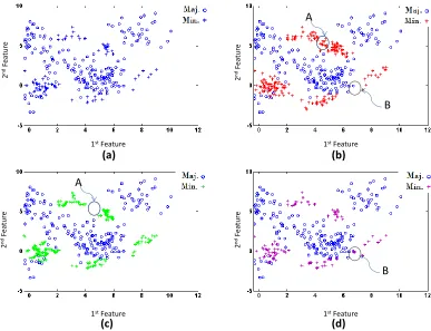
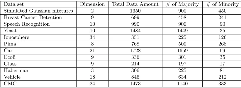
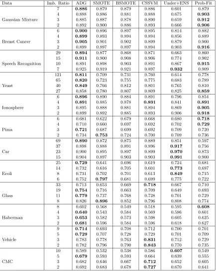
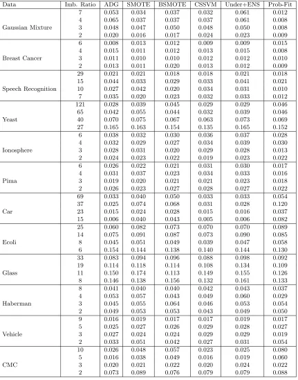
Figure 1 shows a sample of synthetic data generation for a subset of the mixture of Gaussian distributions with an imbalance ratio greater than 6. Comparing region A in plots (b) and (c) in Figure 1 suggests that, for this particular data set, the ADG mechanism is more “space-filling” than that of SMOTE. Comparing region B in plots (b) and (d) shows that the intrusion into the majority space, while attempting to be space-filling, is less of a problem for ADG than that for BSMOTE, which also aims at generating data close to the boundary. Performing this space-filling property within the minority region, is of paramount importance for imbalanced classification in higher dimensions as well. It is not easy to demonstrate this property for the other data sets, as their dimensions are larger than two. The subsequent numerical results, however, support ADG’s potency in imbalanced classification, and we think its strength can be partly attributed to ADG’s ability to maintain the property better than SMOTE and BSMOTE.

4.2 Real Data sets

2 nd F

ea

tu

re

1st _Feature

2

nd F

ea

tu

re

1st _Feature

2

nd F

ea

tu

re

1st _Feature

2

nd F

ea

tu

re

1st _Feature

A

A

B

B

(a) (b)

(c) (d)

Figure 1: Comparing the mechanism of data generation in ADG with SMOTE for an artifi-cial data set: (a) Original imbalanced data; (b) Balanced data after one iteration of ADG; (c) Balanced data after using SMOTE; (d) Balanced data after using BSMOTE. Comparing region A in plots (b) and (c) and region B in plots (c) and (d) shows ADG is more space-filling and intrudes less into the majority space.

Among the aforementioned data sets, not all of them are genuinely imbalanced. In those circumstances, we form the training data sets using a large portion of the majority data and a very small portion of the minority data. Besides, we are interested in observing how different methods perform as a data set becomes more imbalanced. For this purpose, we adjust the degrees of imbalance in a training set, by tuning the ratio of the number of majority points over the number of minority points in the data set. Specifically, for a given imbalance ratio, we first randomly undersample both the majority and the minority data points so that the training data set is constructed with the specified degree of imbalance. This means we obtain new training sets X+

u and Xu− as explained in the beginning of this section, run each algorithm on the training set, and use the remaining data for testing. We repeat this procedure ten times and report the average values as the estimated false alarm rate and detection power. Note that these new X+

Data set Dimension Total Data Amount # of Majority # of Minority

Simulated Gaussian mixtures 2 1350 900 450

Breast Cancer Detection 9 699 458 241

Speech Recognition 10 990 900 90

Yeast 10 1484 1449 35

Ionosphere 34 351 225 126

Pima 8 768 500 268

Car 21 1728 1659 69

Ecoli 9 336 301 35

Glass 9 214 197 17

Haberman 3 306 225 81

Vehicle 18 846 634 212

CMC 24 1473 1140 333

Table 1: Basic properties of data sets

4.3 Results

We represent the performance of each algorithm on each data set using the Area Under Curve (AUC) of the Receiver Operating Characteristic (ROC) plot (Bradley, 1997). In the ROC analysis we plot each (FA, DP) point for a test case in an ROC space in which the FA is on the x-axis and the DP is on the y-axis (Provost et al., 1997). We use the perfcurve

command in MATLAB to generate the ROC curves, once we have computed a sufficient number of (FA, DP) points. Then, we compute AUC as the area under a respective ROC curve. Note that a larger AUC generally denotes better performance.

We apply the six competing methods (ADG included) to the twelve data sets (including the simulated Gaussian mixture data) under different imbalance ratios. We report the average AUC and its standard deviation (both from ten repetitions), instead of the ROC plots themselves. Considering the number of classification methods in comparison, data sets involved, and imbalance ratios used, it is impractical to hope that plotting all ROC curves can produce a clear overall picture. Instead, we present the AUC information in a concise form: Table 2 lists the average values and Table 3 lists the corresponding standard deviations.

As evident in Table 2, ADG provides the largest AUC for most cases, especially under the most imbalanced circumstances of each test instance. Rather than expecting the ROC to suggest the optimal classifier, one may identify the regions or scenarios where a classifier can be recommended (Provost et al., 1997). We find that ADG provides a good balance between the conflicting objectives of reducing the false alarm, while increasing the detection power.

and that no one classifier is dominant for all types of data under all imbalance ratios. The relation between a data structure and the mechanism embedded in the classifiers to handle the imbalanced data is of interest to be understood, but currently there are not enough insights garnered and we leave that issue to future efforts.

The fact that there are no dominating classifiers leads us to ask whether ADG’s perfor-mance is statistically significant compared to the other methods. Considering that we are in presence of several classifiers and several data sets, we need to use a test which ranks classifiers based on their performance, followed by a post hoc analysis. One classical method which we utilize is the Friedman test (Dem˘sar, 2006), a non-parametric method which sorts the algorithms conducted on several data sets. Let ma be the number of algorithms, i.e. classifiers, andmd be the number of data sets. LetRebe anmd×mamatrix of the results listed in Table 2, in which each row represents a data set and each column is a classifier. Considering the average results for each imbalance ratio as produced by one “data set”, we havemd= 48 andma= 6. First, define the matrix Rawhose entries in each row represent the classifier’s rank for that specific data set. Under the null hypothesis that all classifiers are equivalent, i.e. their performance on each data set is identical, the Friedman statistic

F = 12m

d

ma_(ma_{+ 1)} ma

X

`=1

Ra2_` −m

a_(ma_{+ 1)}2 4

!

, (37)

has a Chi-squared distribution with ma−1 degrees of freedom, where Ra` is the average value of column`= 1,2, . . . , ma. Table 4 lists the means for the estimated ranks associated with each method. Figure 2, which presents the post hoc analysis on the ranking data using multiple comparisons, shows the ADG’s ranking is significantly higher than other competing algorithms under the 0.05 level of significance.

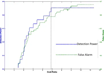
Before concluding this section, we want to briefly discuss the drawbacks of the cost-sensitive approach (Maloof, 2003) and one-class classification (also known as novelty detec-tion) (Park et al., 2010). One major obstacle faced with cost-sensitive methods is how to choose a suitable cost ratio that leads to robust outcomes. Figure 3 shows the detection power and false alarm as a function of cost ratio for the Haberman data where an imbal-ance ratio greater than 3 is used in training. Specifically, the cost ratio denotes the value associated with the box constraint in the SVM for minority data points divided into that value for the majority data points. As Figure 3 shows, the detection power remains almost constant after the cost ratio passes a threshold around 7, yet the false alarm rate continues to increase. Similar evidence has been documented in the literature regarding the lack of robustness in choosing a good cost ratio in the cost-sensitive methods (Byon et al., 2010). This lack of robust performance is one reason why synthetic oversampling is generally more powerful than cost-sensitive methods.

Data Imb. Ratio ADG SMOTE BSMOTE CSSVM Under+ENS Prob-Fit

Gaussian Mixture

7 0.886 0.879 0.879 0.886 0.601 0.879

4 0.888 0.886 0.881 0.888 0.675 0.903

3 0.885 0.887 0.878 0.890 0.659 0.912

2 0.892 0.900 0.886 0.893 0.666 0.906

Breast Cancer

6 0.900 0.896 0.897 0.895 0.814 0.882

4 0.899 0.893 0.894 0.894 0.856 0.889

3 0.905 0.901 0.902 0.899 0.879 0.900

2 0.899 0.897 0.897 0.894 0.903 0.916

Speech Recognition

29 0.894 0.877 0.868 0.871 0.663 0.860

15 0.911 0.900 0.908 0.906 0.774 0.902

10 0.891 0.898 0.903 0.891 0.867 0.915

7 0.925 0.919 0.921 0.897 0.932 0.909

Yeast

121 0.811 0.709 0.731 0.760 0.614 0.778

65 0.820 0.723 0.755 0.775 0.683 0.789

40 0.849 0.766 0.812 0.801 0.765 0.810

27 0.858 0.780 0.807 0.809 0.825 0.859

Ionosphere

6 0.896 0.890 0.884 0.891 0.796 0.854

4 0.891 0.885 0.878 0.891 0.841 0.891

3 0.895 0.888 0.881 0.894 0.869 0.905

2 0.899 0.892 0.885 0.893 0.906 0.918

Pima

6 0.681 0.622 0.679 0.668 0.680 0.718

4 0.710 0.660 0.697 0.692 0.702 0.729

3 0.721 0.687 0.699 0.692 0.709 0.720

2 0.734 0.753 0.724 0.700 0.709 0.736

Car

69 0.890 0.872 0.875 0.889 0.851 0.597

37 0.898 0.888 0.891 0.896 0.917 0.756 23 0.900 0.895 0.897 0.899 0.970 0.873 15 0.904 0.897 0.903 0.903 0.991 0.900

Ecoli

25 0.729 0.641 0.696 0.619 0.724 0.681

14 0.732 0.616 0.705 0.601 0.773 0.697 8 0.731 0.702 0.701 0.613 0.849 0.715 6 0.752 0.797 0.681 0.699 0.775 0.722

Glass

33 0.713 0.653 0.669 0.718 0.667 0.710

19 0.754 0.716 0.663 0.709 0.649 0.693

11 0.779 0.737 0.768 0.728 0.701 0.729

8 0.826 0.896 0.852 0.796 0.808 0.774

Haberman

8 0.602 0.568 0.549 0.518 0.595 0.608

4 0.640 0.543 0.584 0.569 0.586 0.601

3 0.653 0.582 0.573 0.598 0.605 0.625

2 0.681 0.596 0.584 0.596 0.618 0.627

Vehicle

9 0.714 0.693 0.708 0.712 0.700 0.701

5 0.729 0.707 0.728 0.729 0.701 0.709

3 0.783 0.778 0.763 0.831 0.712 0.729 2 0.782 0.796 0.790 0.843 0.770 0.735

CMC

10 0.589 0.532 0.538 0.586 0.607 0.549

5 0.679 0.593 0.593 0.664 0.639 0.555

3 0.682 0.646 0.667 0.712 0.652 0.605 2 0.692 0.683 0.678 0.727 0.670 0.641

Data Imb. Ratio ADG SMOTE BSMOTE CSSVM Under+ENS Prob-Fit

Gaussian Mixture

7 0.053 0.034 0.037 0.032 0.061 0.012 4 0.065 0.037 0.037 0.037 0.061 0.008 3 0.048 0.047 0.050 0.048 0.050 0.008 2 0.020 0.016 0.017 0.024 0.023 0.009

Breast Cancer

6 0.008 0.013 0.012 0.009 0.009 0.015 4 0.015 0.011 0.012 0.013 0.015 0.008 3 0.011 0.010 0.010 0.012 0.012 0.010 2 0.013 0.011 0.020 0.013 0.012 0.009

Speech Recognition

29 0.021 0.021 0.018 0.018 0.021 0.018 15 0.044 0.033 0.029 0.033 0.041 0.021 10 0.027 0.042 0.020 0.034 0.031 0.010 7 0.035 0.020 0.023 0.032 0.033 0.012

Yeast

121 0.028 0.039 0.045 0.029 0.029 0.046 65 0.042 0.055 0.044 0.032 0.039 0.046 40 0.070 0.075 0.067 0.063 0.073 0.069 27 0.165 0.163 0.154 0.135 0.165 0.152

Ionosphere

6 0.038 0.032 0.030 0.036 0.037 0.028 4 0.032 0.029 0.027 0.034 0.039 0.030 3 0.028 0.031 0.020 0.029 0.028 0.013 2 0.024 0.023 0.022 0.019 0.023 0.022

Pima

6 0.026 0.022 0.021 0.031 0.030 0.017 4 0.031 0.037 0.023 0.034 0.033 0.016 3 0.019 0.020 0.021 0.021 0.023 0.018 2 0.026 0.023 0.027 0.028 0.027 0.022

Car

69 0.033 0.040 0.050 0.033 0.033 0.054 37 0.025 0.074 0.068 0.031 0.028 0.120 23 0.015 0.024 0.028 0.015 0.016 0.037 15 0.006 0.040 0.043 0.005 0.006 0.082

Ecoli

25 0.060 0.082 0.073 0.070 0.070 0.089 14 0.075 0.091 0.087 0.073 0.090 0.085 8 0.045 0.051 0.049 0.039 0.047 0.058 6 0.154 0.144 0.138 0.140 0.144 0.130

Glass

33 0.083 0.094 0.096 0.088 0.098 0.092 19 0.114 0.118 0.114 0.108 0.134 0.109 11 0.150 0.174 0.113 0.149 0.155 0.126 8 0.146 0.138 0.156 0.132 0.161 0.133

Haberman

8 0.041 0.040 0.040 0.042 0.043 0.037 4 0.053 0.057 0.043 0.049 0.060 0.029 3 0.045 0.055 0.064 0.046 0.053 0.054 2 0.049 0.053 0.053 0.043 0.049 0.050

Vehicle

9 0.016 0.019 0.017 0.017 0.019 0.017 5 0.025 0.027 0.026 0.029 0.028 0.027 3 0.027 0.024 0.024 0.029 0.029 0.019 2 0.033 0.051 0.042 0.027 0.031 0.054

CMC

10 0.026 0.048 0.057 0.023 0.025 0.080 5 0.016 0.038 0.049 0.016 0.019 0.060 3 0.020 0.021 0.022 0.020 0.024 0.022 2 0.073 0.089 0.076 0.079 0.079 0.088

ADG

SMOTE

BSMOTE

CS-SVM

Under+ENS

Prob-Fit

Detection Power

False Alarm

Classifier ADG SMOTE BSMOTE CSSVM Under+ENS Prob-Fit Mean of Ranking 5.125 2.865 3.104 3.469 2.833 3.604

Table 4: Mean of rankings based on Friedman test

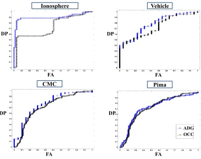
the sparseness of the data, minority data sets still can provide useful information if utilized appropriately. To demonstrate the usefulness of utilizing the minority data, we compare ADG with the OCC method developed in Park et al. (2010) using four sample data sets; this OCC method was proven to provide asymptotically the tightest bound for majority data points. For these four sample data sets, we select the training and test data such that the training data sets have the smallest value of imbalance ratio reported in Table 2. As Figure 4 shows, the OCC could be effective, for instance, duplicating ADG’s performance in the case of Pima data. One drawback is that OCC methods often suffer from a high false alarm rate, while attaining a high detection power (e.g. in the case of the Ionosphere data). When an OCC tries to build the tightest possible closed boundary around the majority data, the result can be an over-tightened boundary, instead of a boundary loose enough to identify all majority data points. On the other hand, in the two-class cases, the existence of minority data points can actually help relax the position of the decision boundary, at least locally where these minority data points are present. For more detailed comparisons of another OCC method with two-class classifiers, the reader may consult (Hempstalk et al., 2008); the results presented there also confirm the argument that if minority data are utilized, one generally observes an improvement in the minority detection.

5. Extension and Error Bounds

In this section, we consider two additional aspects regarding the proposed algorithm. First, we seek to identify bounds on the generalization error for the ADG. Second, we extend the proposed method to deal with the multi-class classification in which a subset of classes has very few observations available in the training stage.

5.1 Bounds on Generalization Error

Generalization error refers to the expected error on test instances coming from the same distribution of the training sample (Rasmussen and Williams, 2006). Specifically, ifx∼ G, whereG is the distribution of the inputx, the generalization error of some decision function h with respect to loss functionL is defined as

Ex{L(h)}, (38)

whereE is the expectation operator.

Let αF denote the optimal value of α obtained by solving optimization problem (3), namely the KFD. Similar to the procedure explained in Section 3 for obtaining the prediction label for ADG, let CU be the same one-dimensional binary classifier used for ADG, trained on the set U = {(h(x`;αF), y`) : x` ∈ X− ∪ X+, ` = 1,2, . . . , n}, where κx is defined

Ionosphere

Vehicle

CMC

Pima

FA DP

FA DP

FA DP

FA DP

OCC ADG

CU isvF, we have the following prediction for a test point xt using the KFD

KFD(xt) =

1 ifh(xt;αF)> vF, −1 ifh(xt;αF)≤vF.

(39)

Consequently, following the total law of probability, we can deduce that the generalization error of KFD is equal to

err_{K =}π−P[h(xt;αF)> vF|yt=−1] +π+P[h(xt;αF)≤vF|yt= 1], (40) whereπi is the prior probability that a point belongs to the class i∈ {−,+}.

Durrant and Kab´an (2012) established an upper bound on this generalization error, under the assumption that the data points of each class follow a Gaussian distribution once mapped to the feature space. Specifically, having a training data set of sizen=l++l− and assuming data in the feature space are normally distributed with mean µ_i and covariance matrixΣfori∈ {−,+}, then for anyρ∈(0,1) the generalization error of KFD is bounded above with probability of at least 1−ρ by ub(l, ρ) where

ub(l, ρ) = X i∈{−,+}

πiΦ

−2

g(¯τ())×Π−

r n li 1 + r 2 nlog 4 ρ , (41) where Π = "s

kµ+−µ−k2 λ_max(Σ) +

n l−l+

tr(Σ) λ_max(Σ)−

s 2n l−l+ log4 ρ # + , (42) g(r) = √ r

1+r for r ∈R, λmax(Σ) is the largest eigenvalue of the covariance matrix, [.]+ = max (0, .), Φ is the CDF of the standard normal distribution, and

¯

τ() = λmax(Σ)

η 1 +

r

n−2 n +

√ n

!2

+τ(Σn), (43)

where = q2 log4_ρ, τ(Σn) denotes the condition number of Σn that is the covariance matrix of the points in a subset of the feature space generated by thenpoints inX−∪ X+_, andηis a regularization constant to ensure non-singularity of the estimate ofΣn. Asg(.) is a monotonic decreasing function onr≥1, a smaller value for ¯τ() suggests a smaller value for the upper bound. Note that assuming the regularization constant η does not need to change as more data points are added to the training set, then the only quantities which affect ¯τ() areτ(Σn) andn.

Note that as the number of observations increases, (41) yields a tighter bound, assuming that all other quantities remain constant. This is in fact what happens in synthetic data generation, especially for ADG, since it generates extra observations at each iteration of the algorithm. The more subtle issue is how the estimated value of the covariance matrix Σ, projected in the Hilbert space generated by the observation, changes with the generation of more data points.

linearly independent, we can havePn=

Xφ_nTXφ_n −1₂

Xφ_nT, whereXφ_n is a matrix whose columns areφ(x`) forx`∈ X−∪ X+. If we add a new observation xn+1 to the training set X−∪ X+_{, we will get the projection matrix P}φ

n+1. See the Appendix for an explanation that as the number of data points increases, the condition number of the covariance matrix of the space generated by the data points in the feature space decreases, which in turn implies we achieve a tighter bound for generalization error using ADG.

In fact, as long as a synthetic data generation mechanism is embedded in a KFD frame-work, as ADG does, we can invoke the above theoretical result on the reduction of the generalization error. Despite the fact that SMOTE and BSMOTE can also be used, note that their data generation mechanisms cannot be integrated with KFD. For this reason, the above error bound result cannot be readily applied to SMOTE and BSMOTE.

5.2 Extension to Multi-class Classification

The methodology presented for the imbalanced two-class classification can be easily ex-tended to cover multi-class classification in which a subset of classes lack sufficient obser-vations for the training stage. Let Xi _={xi

1,xi2, . . . ,xili} ⊂ X denote the training set for

class i ∈ I = {1,2, . . . , Is}, where li2 li1, for i1 ∈ I1, i2 ∈ I2, where I1∪ I2 = I and

I1∩ I2=∅. LetZis ={x

is

lis+1,x

is

lis+2, . . . ,x

is

lis+kis} ⊂ X be the absent data from the

minor-ity classis, and denote eachxlis+kis byz

is

j . For simplicity, consider a case in which the data in each group consist of a single cluster, i.e. C = 1; however, the following algorithm can be readily extended to consider more clusters. Assume that the data are centered around each covariate so they have mean 0. Sequentially solve the following optimization problem to obtain wi for i∈ I:

max

wi

J(wi) = w T i S

φ

Bwi

wT i S

φ

Wwi

, (44)

subject to

wi⊥w`, ∀` < i, (45)

wT_i φ(zis

j )−w T_mφ

is

2

≤δ, (46)

(φ(zis

j )−m

φ

id)

T_(φ(zis

j )−m

φ

ir)≤Λ for j = 1,2, . . . kis, is∈ I2, ir∈ I1, (47)

where Sφ_B and Sφ_W are the between and within class scatter matrices, respectively, in the feature space

Sφ_B =X i∈I

limφi (m

φ

i )T,

Sφ_W =X i∈I

X

x∈Xi

(φ(x)−mφ_i )(φ(x)−mφ_i )T, (48)

and mφ_i = _l1

i

Pli

j=1φ(xij), for i ∈ I. For each minority class in I2, generate kis artificial

points from class ic∈ I2. Similar to the two-class classification problem, use the Represen-ter’s Theorem to replace each wi and φ(zijs)−m

φ

ir as linear combinations of the training

6. Summary

This paper presents an algorithm for solving the two-class classification with imbalanced training data. The difficulty associated with such data structures is that the inadequate number of data points belonging to one class (i.e. minority) leads to the problem that most two-class classification algorithms tend to favor the majority class in labeling test points. To solve the problem, we devise an algorithm that relies on minority data synthesis. At each iteration we solve an optimization which considers more numbers of minority points without explicitly specifying them. Those points affect our decision by forcing the algorithm to set the decision boundary as though the points genuinely existed. We draw samples from the new region to enable a more accurate estimation for the scatter matrices. Using several simulated and real data sets, we compare the performance of the resulting ADG algorithm with the competing methods, CS-SVM, SMOTE, BSMOTE, Under+ENS and Prob-Fit. The results suggest that using ADG is preferable when there is a pronounced data imbalance.

This paper is a first step for developing a data mechanism embedded in a classification algorithm which we proved useful based on empirical evidence. Since the introduction of SMOTE (Chawla et al., 2002), there has been significant attention to synthetic data generation. We suggest however, that more research is needed to understand the relationship between data generation and classification algorithms.

There are a few critical issues which deserve further attention in this regard. First, the impact of the data structure on the data generation mechanism needs to be studied more thoroughly. The current procedure of data generation may not be suitable for all data structures. Certain alterations on the algorithm, based on the knowledge of how the physical system of interest works, can help improve the performance of ADG. Second, ADG can benefit from an investigation into certain assumptions made in the algorithm. One place is on the assumption that the absent data reside in existing clusters. While reasonable, it might be restrictive for some data sets. Another aspect is that in the current iteration of algorithm, we eliminate all artificial data points that fall on the majority side; this appears beneficial in the examples we studied. Whether or not it can be beneficial for all types of data remains unclear. These issues are certainly important and how to address them is an ongoing pursuit.

Acknowledgments

Arash Pourhabib, Yu Ding and Bani K. Mallick were partially supported by grants from NSF (DMS-0914951, CMMI-0926803, and CMMI-1000088) and King Abdullah University of Science and Technology (KUS-CI-016-04). The authors are also grateful of the valuable suggestions made by the editor and referees that greatly improved the paper.

Appendix A.

ζ_{`</sub> for`= 1,2, . . . , n denote the data points mapped to a separable Hilbert space H using a feature map φ, that is ζ_{`</sub> = φ(x`) for ` = 1,2, . . . , n. Suppose Hn is an n dimensional subspace ofHspanned byζ<sub>`}for`= 1,2, . . . , n. Ifζ<sub>`} follow a normal distribution inHwith mean µand covariance matrixΣ, we can have Σnas the projected covariance matrix into the finite dimensional spaceHn. More precisely,Σn=PnΣPT_n, namelyPnis an orthogonal

projection into Hn, where Pn =

Xφ_nTXφ_n −1

2

Xφ_nT and Xφ_n = [ζ<sub>`</sub> :`= 1,2, . . . , n]. We want to show that the condition number ofΣn is larger than or equal to that ofΣn+1.

Without loss of generality, after a rotation and scaling of the data, assume

Xφ_pTXφ_p

=

I, forp∈_N, whereI is the identity matrix of appropriate size. Therefore,

Pn+1 =

Xφ_n+1

T

=

h

(Xφ_n)T|ζT_n+1 i

, (49)

and

λmax(Σn+1) =λmax Pn+1ΣPT_n+1= λmax

"

(Xφ_n)T

ζT_n+1 #

Σ

h

Xφ_n|ζ_n+1 i

!

(50)

= λmax

"

Σn (Xφn)TΣζn+1

ζT_n+1ΣXφ_n ζT_n+1Σζ_n+1 #!

. (51)

Letkζ_n+1k2_:=ζT

n+1Σζn+1. Therefore,

λ_max(Σn+1)≤λmax(Σn) +kζn+1k2, (52) and

λ_min(Σn+1)≥λ_min(Σn) +kζ_n+1k2. (53) Letτ(.) denote the condition number of a matrix, so

τ(Σn+1) = λmax(Σn+1) λ_min(Σn+1) ≤

λ_max(Σn) +kζn+1k2

λ_min(Σn) +kζ_n+1k2 < τ(Σn). (54)

References

Rehan Akbani, Stephen Kwek, and Nathalie Japkowicz. Applying support vector machines to imbalanced datasets. In Proceedings of the fifteenth European Conference on Machine Learning (ECML), pages 39–50. Springer, 2004.

Kurt Anstreicher and Henry Wolkowicz. On Lagrangian relaxation of quadratic matrix constraints. SIAM Journal on Matrix Analysis and Applications, 22(1):41–55, 1998.

Peter J. Bickel and Elizaveta Levina. Some theory for Fishers linear discriminant function, naive Bayes, and some alternatives when there are many more variables than observations. Bernoulli, 10:989–1010, 2004.

Andrew P. Bradley. The use of the area under the ROC curve in the evaluation of machine learning algorithms. Pattern Recognition, 30(7):1145–1159, 1997.

Eunshin Byon, Abhishek K. Shrivastava, and Yu Ding. A classification procedure for highly imbalanced class sizes. IIE Transactions, 42(4):288–303, 2010.

Nitesh V. Chawla, Kevin W. Bowyer, Lawrence O. Hall, and W. Philip Kegelmeyer. SMOTE: Synthetic Minority Over-sampling Technique. Journal of Artificial Intelligence Research, 16:321–357, 2002.

J. J. Chen, C. A. Tsai, J. F. Young, and R. L. Kodell. Classification ensembles for unbal-anced class sizes in predictive toxicology. SAR and QSAR in Environmental Research, 16(6):517–529, 2005.

Janez Dem˘sar. Statistical comparisons of classifiers over multiple data sets. The Journal of Machine Learning Research, 7:1–30, 2006.

Robert J. Durrant and Ata Kab´an. Error bounds for kernel Fisher linear discriminant in Gaussian Hilbert space. In Proceedings of the fifteenth International Conference on Artificial Intelligence and Statistics (AISTATS 2012), volume 22, pages 337–345, 2012.

Charles Elkan. The foundations of cost-sensitive learning. InProceedings of the Seventeenth International Joint Conference on Artificial Intelligence, pages 973–978, 2001.

Chris Fraley and Adrian E Raftery. How many clusters? Which clustering method? Answers via model-based cluster analysis. The Computer Journal, 41(8):578–588, 1998.

Vojtech Franc. The Statistical Pattern Recognition Toolbox, Version 2.11. 2011. URL

http://cmp.felk.cvut.cz/cmp/software/stprtool/index.html.

Alexander Gammerman, Volodya Vovk, and Vladimir Vapnik. Learning by transduction. In Proceedings of the Fourteenth Conference on Uncertainty in Artificial Intelligence, pages 148–155, 1998.

Hui Han, Wen-Yuan Wang, and Bing-Huan Mao. Borderline-SMOTE: A new over-sampling method in imbalanced data sets learning. In Advances in Intelligent Computing, volume 3644 of Lecture Notes in Computer Science, pages 878–887. Springer Berlin Heidelberg, 2005.

Trevor Hastie, Robert Tibshirani, and Jerome Friedman.The Elements of Statistical Learn-ing: Data Mining, Inference, and Prediction, Second Edition. Springer Series in Statistics. Springer New York Inc., New York, NY, USA, 2009.

Kathryn Hempstalk, Eibe Frank, and Ian H. Witten. One-class classification by combining density and class probability estimation. In Walter Daelemans, Bart Goethals, and Katha-rina Morik, editors, Machine Learning and Knowledge Discovery in Databases, volume 5211 of Lecture Notes in Computer Science, pages 505–519. Springer Berlin Heidelberg, 2008.

Thomas Hofmann, Bernhard Sch¨olkopf, and Alexander J. Smola. Kernel methods in ma-chine learning. Annals of Statistics, 36(3):1171–1220, 2008.

Mary Inaba, Naoki Katoh, and Hiroshi Imai. Applications of weighted Voronoi diagrams and randomization to variance-based k-clustering. In Proceedings of the Tenth Annual Symposium on Computational Geometry, pages 332–339. ACM, 1994.

Nathalie Japkowicz. The class imbalance problem: Significance and strategies. In Pro-ceedings of the 2000 International Conference on Artificial Intelligence (ICAI), pages 111–117, 2000.

Tapas Kanungo, David M Mount, Nathan S. Netanyahu, Christine D. Piatko, Ruth Sil-verman, and Angela Y. Wu. An efficient k-means clustering algorithm: Analysis and implementation. IEEE Transactions on Pattern Analysis and Machine Intelligence, 24 (7):881–892, 2002.

Alexander Liu, Joydeep Ghosh, and Cheryl E. Martin. Generative oversampling for mining imbalanced datasets. In International Conference on Data Mining, pages 66–72, 2007.

Xu-Ying Liu, Jianxin Wu, and Zhi-Hua Zhou. Exploratory undersampling for class-imbalance learning. IEEE Transactions on Systems, Man, and Cybernetics, Part B: Cybernetics, 39(2):539–550, 2009.

Marcus A. Maloof. Learning when data sets are imbalanced and when costs are unequal and unknown. In Proceedings of ICML-2003 Workshop on Learning from Imbalanced Data Sets II, 2003.

Sebastian Mika, Gunnar R¨atsch, Jason Weston, Bernhard Sch¨olkopf, and Klaus-Robert M¨ullers. Fisher discriminant analysis with kernels. In Neural Networks for Signal Pro-cessing IX, 1999. Proceedings of the 1999 IEEE Signal ProPro-cessing Society Workshop., pages 41 –48, Aug 1999.

Chiwoo Park, Jianhua Z. Huang, and Yu Ding. A computable plug-in estimator of minimum volume sets for novelty detection. Operations Research, 58(5):1469–1480, Sep 2010.

Dan Pelleg and Andrew Moore. X-means: ExtendingK-means with efficient estimation of the number of clusters. In Proceedings of the Seventeenth International Conference on Machine Learning, pages 727–734. Morgan Kaufmann, 2000.

Carl Edward Rasmussen and Christopher K. I. Williams. Gaussian Processes for Machine Learning. MIT Press, 2006.

Kai Ming Ting. An instance-weighting method to induce cost-sensitive trees. IEEE Trans-actions on Knowledge and Data Engineering, 14(3):659–665, 2002.

Lloyd N. Trefethen and David Bau III. Numerical Linear Algebra. SIAM: Society for Industrial and Applied Mathematics, 1997.

Jakob J. Verbeek, Nikos Vlassis, and Ben Kr¨ose. Efficient greedy learning of Gaussian mixture models. Neural Computation, 15(2):469–485, 2003.

Byron C. Wallace and Issa J. Dahabreh. Class probability estimates are unreliable for imbalanced data (and how to fix them). In IEEE Twelfth International Conference on Data Mining (ICDM), pages 695–704, 2012.

Byron C. Wallace, Kevin Small, Carla E. Brodley, and Thomas A. Trikalinos. Class imbal-ance, redux. InIEEE Eleventh International Conference on Data Mining (ICDM), pages 754–763, 2011.