Causal Discovery with Continuous Additive Noise Models

Causal Discovery with Continuous Additive Noise Models

Jonas Peters∗ [email protected]

Seminar for Statistics, ETH Z¨urich R¨amistrasse 101, 8092 Z¨urich Switzerland

Joris M. Mooij∗ [email protected]

Institute for Informatics, University of Amsterdam Postbox 94323, 1090 GH Amsterdam

The Netherlands

Institute for Computing and Information Sciences, Radboud University Nijmegen Postbox 9010, 6500 GL Nijmegen

The Netherlands

Dominik Janzing [email protected]

Bernhard Sch¨olkopf [email protected]

Max Planck Institute for Intelligent Systems Spemannstraße 38, 72076 T¨ubingen

Germany

Editor:Aapo Hyv¨arinen

Abstract

We consider the problem of learning causal directed acyclic graphs from an observational joint distribution. One can use these graphs to predict the outcome of interventional ex-periments, from which data are often not available. We show that if the observational distribution follows a structural equation model with an additive noise structure, the di-rected acyclic graph becomes identifiable from the distribution under mild conditions. This constitutes an interesting alternative to traditional methods that assume faithfulness and identify only the Markov equivalence class of the graph, thus leaving some edges undirected. We provide practical algorithms for finitely many samples, RESIT (regression with sub-sequent independence test) and two methods based on an independence score. We prove that RESIT is correct in the population setting and provide an empirical evaluation.

Keywords: causal inference, structural equation models, additive noise, identifiability, causal minimality, Bayesian networks

1. Introduction

Many scientific questions deal with the causal structure of a data-generating process. E.g., if we know the reasons why an individual is more susceptible to a disease than others, we can hope to develop new drugs in order to cure this disease or prevent its outbreak. Recent results indicate that knowing the causal structure is also useful for classical machine learning tasks. In the two variable case, for example, knowing which is cause and which is effect has

implications for semi-supervised learning and covariate shift adaptation (Sch¨olkopf et al., 2012).

We consider a p-dimensional random vectorX= (X1, . . . , Xp) with a joint distribution

L(X) and assume that there is a true acyclic causal graph G that describes the data

gen-erating process (see Section 1.3). In this work we address the following problem of causal

inference: given the distribution L(X) we try to infer the graph G. A priori, the causal

graph contains information about the physical process that cannot be found in properties of the joint distribution. One therefore requires assumptions connecting these two worlds. While traditional methods like PC, FCI (Spirtes et al., 2000) or score-based approaches (e.g. Chickering, 2002), that are explained in more detail in Section 2, make assumptions that enable us to recover the graph up to the Markov equivalence class, we investigate a different set of assumptions. If the data have been generated by an additive noise model (see Section 3), we will generically be able to recover the correct graph from the joint distribution.

In the remainder of this section we set up the required notation and definitions for graphs (Section 1.1), briefly introduce Judea Pearl’s do-notation (Section 1.2) and use it to define our object of interest, a true causal graph (Section 1.3). We introduce structural equation models (SEMs) in Section 1.4. After discussing existing methods in Section 2, we provide the main results of this work in Section 3. We prove that for restricted additive noise models, a special class of SEMs, one can identify the graph from the joint distribution. This is possible not only for additive noise models (ANMs) but for all classes of SEMs that are able to identify graphs from a bivariate distribution, meaning they can distinguish between cause and effect. Section 4 proposes algorithms that can be used in practice, when instead of the joint distribution, we are only given i.i.d. samples. These algorithms are tested in Section 5.

This paper builds on the conference papers of Hoyer et al. (2009), Peters et al. (2011b)

and Mooij et al. (2009)1 but extends the material in several aspects. All deliberations

in Section 1.3 about the true causal graph and Example 10 are novel. The presentation of the theoretical results in Section 3 is improved. In particular, we added the motivating Example 26 and Propositions 4 and 29. Example 25 provides a non-identifiable case different

from the linear Gaussian example. Proposition 23 is based on Zhang and Hyv¨arinen (2009)

and contains important necessary conditions for the failure of identifiability. In Corollary 31 we present a novel identifiability result for a class of nonlinear functions and Gaussian noise variables. Proposition 17 proves that causal minimality is satisfied if the structural equations do not contain constant functions. Section 3.3 contains results that guarantee to find the set of correct topological orderings when the assumption of causal minimality is dropped. Theorem 34 proves a conjecture from Mooij et al. (2009) by showing that given a regression and independence oracle the algorithm provided in Mooij et al. (2009) is correct. We propose a new score function for estimating the true directed acyclic graph in Section 4.2 and present two corresponding score-based methods. We provide an extended section on simulation experiments and discuss experiments on real data.

1.1 Directed Acyclic Graphs

We start with some basic notation for graphs. Consider a finite family of random variables

X= (X1, . . . , Xp) with index setV:={1, . . . , p}(we use capital letters for random variables

and bold letters for sets and vectors). We denote their joint distribution byL(X). We write

pX1(x) or simply p(x) for the Radon-Nikodym derivative of L(X1) either with respect to

the Lebesgue or the counting measure and (sometimes implicitly) assume its existence. A

graph G= (V,E) consists of nodesV and edges E ⊆V2 with (v, v)6∈ E for anyv ∈V. In

a slight abuse of notation we identify the nodes (or vertices)j ∈V with the variables Xj,

the context should clarify the meaning. We also consider sets of variablesS⊆Xas a single

multivariate variable. We now introduce graph terminology that we require later. Most of the definitions can be found in Spirtes et al. (2000); Koller and Friedman (2009); Lauritzen (1996), for example.

Let G = (V,E) be a graph with V := {1, . . . , p} and corresponding random variables

X= (X1, . . . , Xp). A graphG1 = (V1,E1) is called asubgraphofGifV1=VandE1 ⊆ E;

we then writeG1 ≤ G. If additionally,E1 6=E, we callG1 a proper subgraphof G.

A node iis called aparent ofj if (i, j)∈ E and achildif (j, i)∈ E. The set of parents

ofj is denoted byPAG_j, the set of its children byCHG_j. Two nodesiandj areadjacentif

either (i, j)∈ E or (j, i)∈ E. We call G fully connectedif all pairs of nodes are adjacent.

We say that there is an undirected edge between two adjacent nodes i and j if (i, j) ∈ E

and (j, i)∈ E. An edge between two adjacent nodes is directed if it is not undirected. We

then writei→j for (i, j)∈ E. Three nodes are called animmorality or av-structureif

one node is a child of the two others that themselves are not adjacent. The skeleton ofG

is the set of all edges without taking the direction into account, that is all (i, j), such that

(i, j)∈ E or (j, i)∈ E.

A path in G is a sequence of (at least two) distinct vertices i1, . . . , in, such that there

is an edge between ik and ik+1 for all k= 1, . . . , n−1. Ifik → ik+1 for all k we speak of

a directed pathfrom i1 toinand call in adescendantof i1. We denote all descendants

of iby DEG_i and all non-descendants of i, excluding i, by NDG_i. In this work, iis neither

a descendant nor a non-descendant of itself. If ik−1 → ik and ik+1 → ik, ik is called a

collider on this path. G is called a partially directed acyclic graph (PDAG) if there

is no directed cycle, i.e., if there is no pair (j,k) such that there are directed paths fromj

tok and from k toj. G is called a directed acyclic graph (DAG) if it is a PDAG and

all edges are directed.

In a DAG, a path between i1 and in is blocked by a set S (with neither i1 nor in

in this set) whenever there is a node ik, such that one of the following two possibilities

hold: 1. ik ∈ S and ik−1 → ik → ik+1 or ik−1 ← ik ← ik+1 or ik−1 ← ik → ik+1 Or 2.,

ik−1 →ik←ik+1 and neitherik nor any of its descendants is inS. We say that two disjoint

subsets of verticesAandBared-separatedby a third (also disjoint) subsetSif every path

between nodes inAandBis blocked byS. Throughout this work, ⊥⊥ denotes (conditional)

independence. The joint distribution L(X) is said to be Markov with respect to the

DAG G if

A,Bd-sep. byC ⇒ A⊥⊥B|C

for all disjoint setsA,B,C. L(X) is said to be faithful to the DAG G if

X

Z

Y c

a

b

X

Z

Y

˜

a

˜_b

G₁ G₂

Figure 1: After fine-tuning the parameters for the two graphs, both models generate the same joint distribution.

for all disjoint sets A,B,C. A distribution satisfies causal minimality with respect

to G if it is Markov with respect to G, but not to any proper subgraph of G. We

de-note by M(G) the set of distributions that are Markov with respect to G: M(G) :=

{L(X) : L(X) is Markov w.r.t. G}. Two DAGs G1 and G2 are Markov equivalent if

M(G₁) = M(G₂). This is the case if and only if G₁ and G₂ satisfy the same set of d

-separations, that means the Markov condition entails the same set of (conditional) inde-pendence conditions. The set of all DAGs that are Markov equivalent to some DAG (a

so-called Markov equivalence class) can be represented by a completed PDAG. This

graph satisfies (i, j) ∈ E if and only if one member of the Markov equivalence class does.

Verma and Pearl (1991) showed that:

Lemma 1 Two DAGs are Markov equivalent if and only if they have the same skeleton and the same immoralities.

Faithfulness is not very intuitive at first glance. We now give an example of a distribution

that is Markov but not faithful with respect to some DAG G1. This is achieved by making

two paths cancel each other and creating an independence that is not implied by the graph structure.

Example 2 Consider the two graphs in Figure 1. Corresponding to the left graph we generate a joint distribution by the following equations. X = NX, Y = aX +NY, Z =

bY +cX+NZ, with normally distributed noise variables NX ∼ N(0, σ2X), NY ∼ N(0, σ2Y)

and NZ ∼ N(0, σZ2) that are jointly independent. This is an example of a linear Gaussian

structural equation model with graph G1 that we formally define in Section 1.4. Now, if a·b+c= 0, the distribution is not faithful with respect toG₁ since we obtainX ⊥⊥Z; more precisely, it is not triangle-faithful (Zhang and Spirtes, 2008).

Correspondingly, we generate a distribution related to graph G2: X = ˜NX, Y = ˜aX+

˜_{bZ + ˜NY, Z = ˜NZ, with all N}˜_{· ∼ N(0, τ}2

·) jointly independent. If we choose τX2 = σ2X,

˜

a=a, τ2

Z =b2σY2 +σZ2, ˜b= (bσ2Y)/(b2σY2 +σ2Z) and τY2 =σ2Y −(b2σY4)/(b2σY2 +σZ2), both

models lead to the covariance matrix

Σ =





σ2_X aσ2_X 0

aσ_X2 a2σ_X2 +σ2_Y bσ_Y2

0 bσ2_Y b2σ_Y2 +σ_Z2





The distribution from Example 2 is faithful with respect to G₂, but not with respect to

G1. Nevertheless, for both models, causal minimality is satisfied if none of the parameters

vanishes: the distribution is not Markov to any proper subgraph ofG₁ orG₂ since removing

an arrow would correspond to a new (conditional) independence that does not hold in the

distribution. Note that G2 is not a proper subgraph of G1. In general, causal minimality is

weaker than faithfulness:

Remark 3 If L(X) is faithful with respect to G, then causal minimality is satisfied.

This is due to the fact that any two nodes that are not directly connected by an edge can

bed-separated. Another, equivalent formulation of causal minimality reads as follows:

Proposition 4 Consider the random vector X = (X1, . . . , Xp) and assume that the joint

distribution has a density with respect to a product measure. Suppose that L(X) is Markov with respect to G. Then L(X) satisfies causal minimality with respect to G if and only if

∀Xj ∀Y ∈PAG_j we have that Xj 6⊥⊥Y |PAG_j \ {Y}.

Proof See Appendix A.1.

1.2 Intervention Distributions2

Given a directed acyclic graph (DAG) G, Pearl (2009) introduces the do-notation as a

mathematical description of interventional experiments. More precisely, do(Xj = ˜p(xj))

stands for setting the variableXj randomly according to the distribution ˜p(xj), irrespective

of its parents, while not interfering with any other variable. Formally:

Definition 5 LetX= (X1, . . . , Xp)be a collection of variables with joint distributionL(X)

that we assume to be absolutely continuous with respect to the Lebesgue measure or the counting measure (i.e., there exists a probability density function or a probability mass function). Given a DAG G over X, we define the intervention distribution do(Xj = ˜p(xj))

of X1, . . . , Xp by

p x1, . . . , xp|do(Xj = ˜p(xj))

:=

p Y

i6=j

p(xi|xPAi)·p˜(xj)

if p(x1, . . . , xp) >0 and zero otherwise. Here p˜(xj) is either a probability density function

or a probability mass function. Similarly, we can intervene at different nodes at the same time by defining the intervention distributiondo(Xj = ˜p(xj), j ∈J) for J⊆V as

p x1, . . . , xp|do(Xj = ˜p(xj), j ∈J)

:=Y

i /∈J

p(xi|xPA_i)·

Y

j∈J

˜

p(xj)

if p(x1, . . . , xp)>0 and zero otherwise.

Here, xPA_i denotes the tuple of all xj for Xj being a parent of Xi in G. Pearl (2009)

introduces Definition 5 with the special case of ˜p(xj) =δxj,x˜j, where δxj,˜xj = 1 if xj = ˜xj

and δxj,x˜j = 0 otherwise; this corresponds to a point mass at ˜xj. For more details onsoft

interventions, see Eberhardt and Scheines (2007). Note that in general:

p(x1, . . . , xp|do(Xj = ˜xj))6=p(x1, . . . , xp|Xj = ˜xj).

The expression p x1, . . . , xp|do(Xj = ˜xj, j ∈J)

yields a distribution overX1, . . . , Xp. If

we are only interested in computing the marginal p xi|do(Xj = ˜xj)), where Xi is not a

parent ofXj, we can use the parent adjustment formula (Pearl, 2009, Theorem 3.2.2)

p(xi|do(Xj = ˜xj)) = X

xPA_j

p(xi|x˜j, xPA_j)p(xPA_j). (1)

1.3 True Causal Graphs2

In this section we clarify what we mean by a true causal graph G_c. In short, we use this

term if the results of randomized studies are determined byGc and the observational joint

distribution. This means that the graph and the observational joint distribution lead to causal effects that one observes in practice. Two important restrictive assumptions that we

make throughout this work areacyclicity (the absence of directed cycles, in other words, no

causal feedback loops are allowed) and causal sufficiency (the absence of hidden variables

that are a common cause of at least two observed variables).

Definition 6 Assume we are given a distribution L(X) over X1, . . . , Xp and distributions L_{do(Xj= ˜p(xj),j∈J)}(X) for all J ⊆ V = {1, . . . , p} (think of the variables Xj having been

randomized). We then call the graph Gc a true causal graph for these distributions if • Gc is a directed acyclic graph;

• the distribution L(X) is Markov with respect to G_c;

• for allJ⊆Vandp˜(xj)withj∈Jthe distributionLdo(Xj= ˜p(xj),j∈J)(X)coincides with

p x1, . . . , xp|do(Xj = ˜p(xj), j∈J)

, computed from Gc as in Definition 5.

Definition 6 is purely mathematical if one considers L_do(X

j= ˜p(xj),j∈J)(X) as an abstract

family of given distributions. But it is a small step to make the relation to the “real

world”. We callG_c the true causal graphof a data generating processif it is the true causal

graph for the distributionsL(X) andL_do(X

j= ˜p(xj),j∈J)(X), where the latter are obtained by

randomizing Xj according to ˜p(xj). In some situations, the precise design of a randomized

experiment may not be obvious. While most people would agree on how to randomize over medical treatment procedures, there is probably less agreement how to randomize over the tolerance of a person (does this include other changes of his personality, too?). Only sometimes, this problem can be resolved by including more variables and taking a less coarse-grained point of view. We do not go into further detail since we believe that this would require philosophical deliberations, which lie beyond the scope of this work. Instead, we may explicitly add the requirement that “most people agree on what a randomized experiment should look like in this context”.

Proposition 7 Assume L(X1, . . . , Xp) has a density and consider all true causal DAGs

G:={Gc,1, . . . ,Gc,m} of X1, . . . , Xp. Then there is a partial order onG using the subgraph property ≤ as an ordering. This ordering has a least element G_c, i.e., G_c ≤ G_c,i for all i. This element G_c is the unique true causal DAG such that L(X) satisfies causal minimality with respect to Gc.

Proof See Appendix A.2

We now briefly comment on a true causal graph’s behavior when some of the variables from the joint distribution are marginalized out.

Example 8 (i) If X ← Z → Y is the only true causal graph for X, Y and Z, there is no true causal graph for the variables X and Y (the do-statements do not coincide).

(ii) Assume that the graph X → Y → Z with additional X → Z is the only true causal graph forX, Y andZ and assume thatL(X, Y, Z) is faithful with respect to this graph. Then, the only true causal graph for the variables X and Z is X→Z.

(iii) If the situation is the same as in (ii) with the difference that X⊥⊥Z (i.e., L(X, Y, Z)

is not faithful with respect to the true causal graph), the empty graph and Z ←X are also true causal graphs for X and Z.

Latent projections (Verma and Pearl, 1991) provide a formal way to obtain a true causal graph for marginalization. Cases (ii) and (iii) show that there are no purely graphical

criteria that provide theminimaltrue causal graph described in Proposition 7.

The results presented in the remainder of this paper can be understood without causal interpretation. Using these techniques to infer a true causal graph, however, requires the

assumption that such a true causal DAG G_c for the observed distribution of X1, . . . , Xp

exists. This includes the assumption that all “relevant” variables have been observed,

sometimes called causal sufficiency, and that there are no feedback loops.

Richardson and Spirtes (2002) introduce a representation of graphs (so-called Maximal Ancestral Graphs, or MAGs) with hidden variables that is closed under marginalization and conditioning. The FCI algorithm (Spirtes et al., 2000) exploits the conditional in-dependences in the data to partially reconstruct the graph. Other work concentrates on hidden variables in structural equation models (e.g., Hoyer et al., 2008; Janzing et al., 2009; Silva and Ghahramani, 2009).

1.4 Structural Equation Models

A structural equation model (SEM) (also called a functional model) is defined as a tuple

(S,L(N)), whereS = (S1, . . . , Sp) is a collection ofp equations

Sj : Xj =fj(PAj, Nj), j= 1, . . . , p (2)

and L(N) =L(N1, . . . , Np) is the joint distribution of the noise variables, which we require

to be jointly independent, i.e., L(N) is a product distribution. We consider SEMs only

for real-valued random variables X1, . . . , Xp. The graph of a structural equation model is

each variable Xk occurring on the right-hand side of equation (2) to Xj. We henceforth

assume this graph to be acyclic. According to the notation defined in Section 1.1,PA_j are

the parents of Xj.

The PA_j can be considered as the direct causes ofXj. An SEM specifies how thePAj

affect Xj. Note that in physics (chemistry, biology, . . . ), we would usually expect that

such causal relationships occur in time, and are governed by sets of coupled differential equations. Under certain assumptions such as stable equilibria, one can derive an SEM that describes how the equilibrium states of such a dynamical system will react to physical interventions on the observables involved (Mooij et al., 2013). We do not deal with these issues in the present paper but take the SEM as our starting point instead. We formulate the identifiability results without the notion of causality.

Pearl (2009) shows in Theorem 1.4.1 that the lawL(X) generated by an SEM is Markov

with respect to its graph. Reversely, there always exists an SEM that models a given

distribution.3

Proposition 9 Consider X1, . . . , Xp and let L(X) have a strictly positive density with

respect to the Lebesgue measure and assume it is Markov with respect to G. Then there exists an SEM (S,L(N)) with graph G that generates the distribution L(X).

Proof See Appendix A.3.

Structural equation models contain strictly more information than their corresponding graph and law and hence also more information than the family of all intervention dis-tributions together with the observational distribution. This information sometimes helps to answer counterfactual questions, as shown in the following example.

Example 10 Let N1, N2 ∼ Ber(0.5) and N3 ∼U({0,1,2}), such that the three variables

are jointly independent. That is, N1, N2 have a Bernoulli distribution with parameter 0.5

and N3 is uniformly distributed on {0,1,2}. We define two different SEMs, first consider:

SA=  



X1=N1 X2=N2

X3= (1N3>0·X1+ 1N3=0·X2)·1X16=X2 +N3·1X1=X2.

IfX1andX2have different values, depending onN3 we either chooseX3=X1 orX3 =X2.

Otherwise X3 =N3. Now, SB differs from SA only in the latter case:

SB =  



X1=N1 X2=N2

X3= (1N3>0·X1+ 1N3=0·X2)·1X16=X2 + (2−N3)·1X1=X2.

It can be checked that both SEMs generate the same observational distribution, which sat-isfies causal minimality with respect to the graph X1 → X3 ←X2. They also generate the

same intervention distributions, for any possible intervention. But the two models differ in a counterfactual statement.4 Suppose, we have seen a sample (X1, X2, X3) = (1,0,0) and

3. A similar but weaker statement than Proposition 9 can be found in Druzdzel and van Leijen (2001); Janzing and Sch¨olkopf (2010).

we are interested in the counterfactual question, what X3 would have been if X1 had been

0. From both SA and SB it follows that N3 = 0, and thus the two SEMs “predict” different

values for X3 under a counterfactual change ofX1.

If we want to use an estimated SEM to predict counterfactual questions, this example

shows that we require assumptions that let us distinguish between S_A orS_B. In this work

we exploit the additive noise assumption to infer thestructure of an SEM. We do not claim

that we can predict counterfactual statements.

Structural equation models have been used for a long time in fields like agriculture or social sciences (e.g., Wright, 1921; Bollen, 1989). Model selection, for example, was done by fitting different structures that were considered as reasonable given the prior knowledge about the system. These candidate structures were then compared using goodness of fit tests. In this work we instead consider the question of identifiability, which has not been addressed until more recently.

Problem 11 (population case) We are given a distribution L(X) =L(X1, . . . , Xp) that

has been generated by an (unknown) structural equation model with graph G₀; in particular,

L(X) is Markov with respect toG0. Can the (observational) distribution L(X) be generated

by a structural equation model with a different graph G 6=G₀? If not, we callG₀ identifiable from L(X).

In general,G₀is not identifiable fromL(X): the joint distributionL(X) is certainly Markov

with respect to a lot of different graphs, e.g., to all fully connected acyclic graphs. Propo-sition 9 states the existence of corresponding SEMs. What can be done to overcome this indeterminacy? The hope is that by using additional assumptions one obtains restricted models, in which we can identify the graph from the joint distribution. Considering

graph-ical models, we see in Section 2.1 how the assumption that L(X) is Markov and faithful

with respect toG₀ leads to identifiability of the Markov equivalence class ofG₀. Considering

SEMs, we see in Section 3 that additive noise models as a special case of restricted SEMs even lead to identifiability of the correct DAG. Also Section 2.3 contains such a restriction based on SEMs.

2. Alternative Methods

We briefly describe some existing methods and provide references for more details.

2.1 Estimating the Markov Equivalence Class: Independence-Based Methods

Conditional independence-based methods like the PC algorithm and the FCI algorithm

(Spirtes et al., 2000) assume that L(X) is Markov and faithful with respect to the correct

graphG₀ (that meansall conditional independences in the joint distribution are entailed by

The first step of the PC algorithm determines the variables that are adjacent. One

therefore has to test whether two variables are dependent givenanyother subset of variables.

The PC algorithm exploits a very clever procedure to reduce the size of the condition set. In the worst case, however, one has to perform conditional independence tests with

conditioning sets of up top−2 variables (wherep is the number of variables in the graph).

Although there is recent work on kernel-based conditional independence tests (Fukumizu et al., 2008; Zhang et al., 2011), such tests are difficult to perform in practice if one does not restrict the variables to follow a Gaussian distribution, for example (e.g., Bergsma, 2004).

To prove consistency of the PC algorithm one does not only require faithfulness, but

strong faithfulness (Zhang and Spirtes, 2003; Kalisch and B¨uhlmann, 2007). Uhler et al.

(2013) argue that this is a restrictive condition. Since parts of faithfulness can be tested given the data (Zhang and Spirtes, 2008), the condition may be weakened.

From our perspective independence-based methods face the following challenges: (1) We can identify the correct DAG only up to Markov equivalence classes. (2) Conditional independence testing, especially with a large conditioning set, is difficult in practice. (3) Simulation experiments suggest, that in many cases, the distribution is close to unfaithful-ness. In these cases there is no guarantee that the inferred graph(s) will be close to the original one.

2.2 Estimating the Markov Equivalence Class: Score-Based Methods

Although the roots for score-based methods for causal inference may date back even further, we mainly refer to Geiger and Heckerman (1994), Heckerman (1997) and Chickering (2002)

and references therein. Given the dataDfrom a vectorXof variables, i.e.,ni.i.d. samples,

the idea is to assign a scoreS(D,G) to each graphG and search over the space of DAGs for

the best scoring graph:

ˆ

G := argmax

GDAG overX

S(D,G). (3)

There are several possibilities to define such a scoring function. Often a parametric model is assumed (e.g., linear Gaussian equations or multinomial distributions), which introduces

a set of parameters θ∈Θ.

From a Bayesian point of view, we may define priors ppr(G) and ppr(θ) over DAGs and

parameters and consider the log posterior as a score function, or equivalently (note that

p(D) is constant over all DAGs):

S(D,G) := logppr(G) + logp(D|G),

wherep(D|G) is the marginal likelihood

p(D|G) =

Z

Θ

p(D|G, θ)·ppr(θ)dθ.

In this case, ˆGdefined in (3) is the mode of the posterior distribution, which is usually called

be averaged over all graphs to get a posterior of the hypothesis about the existence of a specific edge, for example.

In the case of parametric models, we call two graphs G₁ and G₂ distribution equivalent

if for each parameter θ1 ∈ Θ1 there is a corresponding parameter θ2 ∈ Θ2, such that

the distribution obtained from G1 in combination with θ1 is the same as the distribution

obtained from graphG₂ withθ2, and vice versa. It is known that in the linear Gaussian case

(or for unconstrained multinomial distributions) two graphs are distribution-equivalent if

and only if they are Markov equivalent. One may therefore argue thatp(D|G1) and p(D|G2)

should be the same for Markov equivalent graphsG1 andG2. Heckerman and Geiger (1995)

discuss how to choose the prior over parameters accordingly.

Instead, we may consider the maximum likelihood estimator ˆθin each graph and define

a score function by using a penalty, e.g., the Bayesian Information Criterion (BIC):

S(D,G) = logp(D|θ,ˆ G)−d

2logn ,

wheren is the sample size anddthe dimensionality of the parameterθ.

Since the search space of all DAGs is growing super-exponentially in the number of vari-ables (e.g., Chickering, 2002), greedy search algorithms are applied to solve equation (3): at each step there is a candidate graph and a set of neighboring graphs. For all these neigh-bors one computes the score and considers the best-scoring graph as the new candidate. If none of the neighbors obtains a better score, the search procedure terminates (not knowing whether one obtained only a local optimum). Clearly, one therefore has to define a

neigh-borhood relation. Starting from a graphG, we may define all graphs as neighbors from G

that can be obtained by removing, adding or reversing one edge. In the linear Gaussian case, for example, one cannot distinguish between Markov equivalent graphs. It turns out that in those cases it is beneficial to change the search space to Markov equivalence classes instead of DAGs. The greedy equivalence search (GES) (Meek, 1997; Chickering, 2002) starts with the empty graph and consists of two-phases. In the first phase, edges are added until a local maximum is reached; in the second phase, edges are removed until a local maximum is reached, which is then given as an output of the algorithm. Chickering (2002) proves consistency of this method by using consistency of the BIC (Haughton, 1988).

2.3 Estimating the DAG: LiNGAM

Kano and Shimizu (2003) and Shimizu et al. (2006) propose an inspiring method exploiting

non-Gaussianity of the data.5 Although their work covers the general case, the idea is

maybe best understood in the case of two variables:

Example 12 Suppose

Y =φX +N, N ⊥⊥X ,

where X and N are normally distributed. It is easy to check that

X= ˜φY + ˜N , N˜ ⊥⊥Y .

with φ˜= _φ2_varφvar_(X(X₎₊)_σ2 6= _φ1 and N˜ =X−φY˜ .

If we consider non-Gaussian noise, however, the structural equation model becomes identi-fiable.

Proposition 13 Let X andY be two random variables, for which

Y =φX+N, N ⊥⊥X, φ6= 0

holds. Then we can reverse the process, i.e., there exists ψ∈_R and a noiseN˜, such that

X=ψY + ˜N , N˜ ⊥⊥Y ,

if and only if X and N are Gaussian distributed.

Shimizu et al. (2006) were the first to report this result. They prove it even for more than two variables using Independent Component Analysis (ICA) (Comon, 1994, Theorem 11),

which itself is proved using the Darmois-Skitoviˇc theorem (Skitoviˇc, 1954, 1962; Darmois,

1953). Alternatively, Proposition 13 can be proved directly using the Darmois-Skitoviˇc

theorem (e.g., Peters, 2008, Theorem 2.10).

Theorem 14 (Shimizu et al., 2006) Assume a linear SEM with graphG0 Xj =

X

k∈PAG_j0

βjkXk+Nj, j= 1, . . . , p , (4)

where all Nj are jointly independent and non-Gaussian distributed. Additionally, for each

j∈ {1, . . . , p} we require βjk 6= 0 for all k∈PAGj0. Then, the graphG0 is identifiable from

the joint distribution.

The authors call this model a linear non-Gaussian acyclic model (LiNGAM) and provide a practical method based on ICA that can be applied to a finite amount of data. Later,

improved versions of this method have been proposed in Shimizu et al. (2011); Hyv¨arinen

and Smith (2013).

2.4 Estimating the DAG: Gaussian SEMs with Equal Error Variances

There is another deviation from linear Gaussian SEMs that makes the graph identifiable.

Peters and B¨uhlmann (2014) show that restricting the noise variables to have the same

variance is sufficient to recover the graph structure.

Theorem 15 (Peters and B¨uhlmann, 2014) Assume an SEM with graphG0 Xj =

X

k∈PAG0 j

βjkXk+Nj, j= 1, . . . , p , (5)

where all Nj are i.i.d. and follow a Gaussian distribution. Additionally, for each j ∈ {1, . . . , p} we require βjk 6= 0for all k∈PAG_j0. Then, the graph G0 is identifiable from the

For estimating the coefficients βjk and the error variance σ2, Peters and B¨uhlmann (2014)

propose to use a penalized maximum likelihood method (BIC). For optimization they pro-pose a greedy search algorithm in the space of DAGs. Rescaling the variables changes the variance of the error terms. Therefore, in many applications model (5) cannot be sensibly applied. The BIC criterion, however, always allows us to compare the method’s score with the score of a linear Gaussian SEM that uses more parameters and does not make the assumption of equal error variances.

3. Identifiability of Continuous Additive Noise Models

Recall that equation (2) defines the general form of an SEM:Xj =fj(PAj, Nj), j = 1, . . . , p

with jointly independent variables Ni. We have seen that these models are too general to

identify the graph (Proposition 9). It turns out, however, that constraining the function class leads to identifiability. As a first step we restrict the form of the function to be additive with respect to the noise variable. (Throughout this section we assume that all random variables are absolutely continuous with respect to the Lebesgue measure. Peters et al. (2011a) provide an extension for variables that are absolutely continuous with respect to the counting measure.)

Definition 16 We define a continuous additive noise model (ANM) as a tuple (S,L(N)), where S = (S1, . . . , Sp) is a collection of p equations

Sj : Xj =fj(PAj) +Nj, j= 1, . . . , p , (6)

where the PA_j correspond to the direct parents of Xj, and the noise variables Nj have a

strictly positive density (with respect to the Lebesgue measure) and are jointly independent. Furthermore, we assume that the corresponding graph is acyclic.

For these models causal minimality reduces to the condition that each function fj is not

constant in any of its arguments:

Proposition 17 Consider a distribution generated by a model (6) and assume that the functions fj are not constant in any of its arguments, i.e., for allj and i∈PAj there are

some x_PA

j\{i} and somexi6=x

0

i such that

fj(xPAj\{i}, xi)6=fj(xPAj\{i}, x

0 i).

Then the joint distribution satisfies causal minimality with respect to the corresponding graph. Conversely, if there is a j and i such that fj(xPAj\{i},·) is constant, causal

mini-mality is violated.

Proof See Appendix A.4

3.1 Bivariate Additive Noise Models

We now add another assumption about the form of the structural equations.

Definition 18 Consider an additive noise model (6)with two variables, i.e., the two equa-tionsXi=Ni and Xj =fj(Xi) +Nj with{i, j}={1,2}. We call this SEM an identifiable

bivariate additive noise model if the triple (fj,L(Xi),L(Nj)) satisfies Condition 19.

Condition 19 The triple (fj,L(Xi),L(Nj)) does not solve the following differential

equa-tion for allxi, xj withν00(xj−f(xi))f0(xi)6= 0:

ξ000 =ξ00

−ν 000_f0 ν00 +

f00 f0

−2ν00f00f0+ν0f000+ν

0_ν000_f00_f0 ν00 −

ν0(f00)2

f0 , (7)

Here, f := fj, and ξ := logpXi and ν := logpNj are the logarithms of the strictly positive

densities. To improve readability, we have skipped the arguments xj−f(xi), xi, and xi for

ν, ξ, and f and their derivatives, respectively.

Zhang and Hyv¨arinen (2009) even allow for a bijective transformation of the data, i.e.,

Xj = gj(fj(Xi) +Nj) and obtain a similar differential equation as (7). As the name in

Definition 18 already suggests, we have identifiability for this class of SEMs.

Theorem 20 LetL(X) =L(X1, X2)be generated by an identifiable bivariate additive noise

model with graphG0 and assume causal minimality, i.e., a non-constant functionfj

(Propo-sition 17). Then, G₀ is identifiable from the joint distribution.

Proof The proof of Hoyer et al. (2009) is reproduced in Appendix A.5.

Intuitively speaking, we expect a “generic” triple (fj,L(Xi),L(Nj)) to satisfy Condition 19.

The following proposition presents one possible formalization. After fixing (fj,L(Nj)) we

consider the space of all distributionsL(Xi) such that Condition 19 is violated. This space is

contained in a three dimensional space. Since the space of continuous distributions is infinite dimensional, we can therefore say that Condition 19 is satisfied for “most distributions”

L(Xi).

Proposition 21 If for a fixed pair (fj,L(Nj)) there exists xj ∈ R such that ν00(xj −

f(xi))f0(xi)= 06 for all but a countable set of points xi ∈R, the set of all L(Xi) for which

(fj,L(Xi),L(Nj))does not satisfy Condition 19 is contained in a 3-dimensional space.

Proof See Appendix A.6.

The condition ν00(xj −f(xi))f0(xi) 6= 0 holds for all xi if there is no interval where f is

constant and the logarithm of the noise density is not linear, for example. In the case of Gaussian variables, the differential equation (7) simplifies. We thus have the following result.

Corollary 22 IfXi andNj follow a Gaussian distribution and(fj,L(Xi),L(Nj))does not

Proof See Appendix A.7.

Although non-identifiable cases are rare, the question remains when identifiability is

vi-olated. Zhang and Hyv¨arinen (2009) prove that non-identifiable additive noise models

necessarily fall into one out of five classes.

Proposition 23 (Zhang and Hyv¨arinen, 2009) ConsiderXj =fj(Xi) +Nj with fully

supported noise variableNj that is independent ofXi and three times differentiable function

fj. Let further _dxd_ifj(xi) d

2

dx2 j

logpNj(xj) = 0 only at finitely many points (xi, xj). If there is

a backward model, i.e., we can write Xi = gi(Xj) +Mi with Mi independent of Xj, then

one of the following must hold.

I. Xi is Gaussian, Nj is Gaussian and fj is linear.

II. Xi is log-mix-lin-exp, Nj is log-mix-lin-exp and fj is linear.

III. Xi is log-mix-lin-exp, Nj is one-sided asymptotically exponential and fj is strictly

monotonic with f_j0(xi)→0 as xi→ ∞ or as xi→ −∞.

IV. Xi is log-mix-lin-exp, Nj is generalized mixture of two exponentials andfj is strictly

monotonic with f_j0(xi)→0 as xi→ ∞ or as xi→ −∞.

V. Xi is generalized mixture of two exponentials,Nj is two-sided asymptotically

exponen-tial and fj is strictly monotonic with fj0(xi)→0 as xi → ∞ or as xi → −∞.

Precise definitions can be found in Appendix A.8. In particular, we obtain identifiability

whenever the function fj is not injective. Proposition 23 states that belonging to one of

these classes is a necessary condition for non-identifiability. We now show sufficiency for two classes. The linear Gaussian case is well-known and easy to prove.

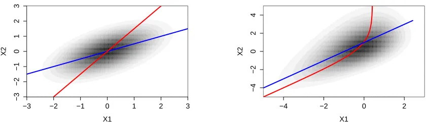
Example 24 LetX2=aX1+N2 with independentN2 ∼ N(0, σ2)andX1∼ N(0, τ2). We

can then consider all variables in L2 and project X1 onto X2. This leads to an orthogonal

decompositionX1 = ˜aX2+ ˜N1. Since for jointly Gaussian variables uncorrelatedness implies

independence, we obtain a backward additive noise model. Figure 2 (left) shows the joint density and the functions for the forward and backward model.

We also give an example of a nonidentifiable additive noise model with non-Gaussian dis-tributions; the forward model is described by case II, and the backward model by case IV:

Example 25 LetX2 =aX1+b+N2 with independent log-mix-lin-expN2 andX1, i.e., we

have the log-densities

ξ(x) = logpX1(x) =c1exp(c2x) +c3x+c4

and

ν(n) = logpN2(n) =γ1exp(γ2n) +γ3n+γ4.

Then X2 is a generalized mixture of exponential distributions. If and only if c2 = −aγ2

and c3 6= aγ3 we obtain a valid backward model X1 = ˜f1(X2) + ˜N1 with log-mix-lin-exp

˜

N1. Again, Figure 2 (right) shows the joint distribution over X1 and X2 and forward and

−3 −2 −1 0 1 2 3

−3

−2

−1

0

1

2

3

X1

X2

−4 −2 0 2

−4

−2

0

2

4

X1

X2

Figure 2: Joint density over X1 and X2 for two non-identifiable examples. The left panel

shows Example 24 (linear Gaussian case) and the right panel shows Example 25 (the latter plot is based on kernel density estimation). The blue function

corre-sponds to the forward modelX2=f2(X1) +N2, the red function to the backward

modelX1= ˜f1(X2) + ˜N1.

Proof See Appendix A.9.

Example 25 shows how parameters of function, input and noise distribution have to be “fine-tuned” to yield non-identifiability (Janzing and Steudel, 2010).

It can be shown that bivariate identifiability even holds generically when feedback is

allowed (i.e., if both X → Y and Y → X), at least when assuming noise and input

distributions to be Gaussian (Mooij et al., 2011).

3.2 From Bivariate to Multivariate Models

It turns out that Condition 19 also suffices to prove identifiability in the multivariate case.

Assume we are given p structural equations Xj = fj(PAj) +Nj as in (6). If we fix all

arguments of the functions fj except for one parent and the noise variable, we obtain a

bivariate model. One may expect that it suffices to put restrictions like Condition 19 on this triple of function, input and noise distribution. This is not the case.

Example 26 Consider the following SEM

X1 =N1, X2 =f2(X1) +N2, X3 =f3(X1) +a·X2+N3

with N1 ∼tν=3, N2 ∼ N(0, σ22) and N3 ∼ N(0, σ23), i.e., N1 is t-distributed with 3 degrees

of freedom andN2 andN3 are normally distributed. X2 and X3 are non-Gaussian but X3|X1=x1 =c+a·X2|X1=x1 +N3

is a linear Gaussian equation for all x1. We can revert this equation and obtain the same

joint distribution by an SEM of the form

for some g1, g2 and M1 ∼tν=3, M2∼ N(0,σ˜22) and M3 ∼ N(0,σ˜23). Thus, the DAG is not

identifiable from the joint distribution.

Instead, we need to put restrictions on conditional distributions.

Definition 27 Consider an additive noise model (6) with p variables. We call this SEM

a restricted additive noise model if for all j ∈ V, i ∈ PA_j and all sets S ⊆ V with

PA_j\ {i} ⊆S⊆ND_j\ {i, j}, there is anxS with pS(xS)>0, s.t.

fj(xPA_j\{i}, · |{z}

Xi

),L(Xi|XS=xS),L(Nj)

satisfies Condition 19. Here, the underbrace indicates the input component offj for variable

Xi. In particular, we require the noise variables to have non-vanishing densities and the

functions fj to be continuous and three times continuously differentiable.

Assuming causal minimality, we can identify the structure of the SEM from the distribution.

Theorem 28 Let L(X) =L(X1, . . . , Xp) be generated by a restricted additive noise model

with graph G0 and let L(X) satisfy causal minimality with respect to G0, i.e., the functions fj are not constant (Proposition 17). Then, G0 is identifiable from the joint distribution. Proof See Appendix A.11.

Our proof of Theorem 28 contains a graphical statement that turns out to be a main argument for proving identifiability for Gaussian models with equal error variances (Peters

and B¨uhlmann, 2014). We thus state it explicitly as a proposition.

Proposition 29 Let G andG0 _{be two different DAGs over variables X.}

(i) Assume that L(X) has a strictly positive density and satisfies the Markov condition and causal minimality with respect to G and G0. Then there are variables L, Y ∈ X

such that for the sets Q:=PAG_L\ {Y}, R:=PA_YG0\ {L} and S:=Q∪R we have

• Y →Lin G and L→Y in G0

• S⊆NDG_L\ {Y} andS⊆NDG_Y0\ {L}

(ii) In particular, ifL(X)is Markov and faithful with respect toGandG0 (i.e., both graphs belong to the same Markov equivalence class), there are variables L, Y such that

• Y →L in G and L→Y in G0 • PAG_L\ {Y}=PAG_Y0 \ {L} Proof See Appendix A.12.

If the distribution is Markov and faithful with respect to the underlying graph it is known that we can recover the correct Markov equivalence class. Chickering (1995) proves that two graphs within this Markov equivalence class can be transformed into each other by a sequence of so-called covered edge reversals. This result implies part (ii) of the proposition. Part (i) establishes a similar statement when replacing faithfulness by causal minimality.

Remark 30 Theorem 28 is not limited to restricted additive noise models. Whenever we have a restriction like Condition 19 that ensures identifiability in the bivariate case (The-orem 20), the multivariate version (The(The-orem 28) remains valid. The proof we provide in the appendix stays exactly the same. The algorithms in Section 4, however, use standard regression methods and therefore rely on the additive noise assumption.

The result can therefore be used to prove identifiability of SEMs that are restricted to discrete additive noise models (Peters et al., 2011a) or post-nonlinear additive noise models

(Zhang and Hyv¨arinen, 2009). In the latter model class we allow a bijective nonlinear

distortion: Xj = gj fj(PAj) +Nj

. These models allow for more complicated functional relationships but are harder to fit from empirical data than the additive noise models considered in this work.

We now state a specific identifiability result for Gaussian noise that we believe to consti-tute an important model class for applications. Tamada et al. (2011b) have already used this result for structure learning without giving an identifiability result (see also Tamada et al.,

2011a). More recently, B¨uhlmann et al. (2013) investigate model (8) in a high-dimensional

context. A bivariate version of the following corollary can be found as Lemma 6 in Zhang

and Hyv¨arinen (2009).

Corollary 31 (i) Let L(X) =L(X1, . . . , Xp) be generated by an SEM with

Xj =fj(PAj) +Nj,

with normally distributed noise variablesNj ∼ N(0, σ2j) and three times differentiable

functions fj that are not linear in any component: denote the parents PAj of Xj

by Xk1, . . . , Xk`, then the functionfj(xk1, . . . , xka−1,·, xka+1, . . . , xk`) is assumed to be

nonlinear for alla and some xk1, . . . , xka−1, xka+1, . . . , xk`∈R

`−1_.

(ii) As a special case, let L(X) =L(X1, . . . , Xp) be generated by an SEM with

Xj = X

k∈PAj

fj,k(Xk) +Nj, (8)

with normally distributed noise variablesNj ∼ N(0, σ2j) and three times differentiable,

nonlinear functions fj,k.

In both cases (i) and (ii), we can identify the corresponding graph G0 from the distribution L(X). The statements remain true if the noise distributions for source nodes, i.e., nodes with no parents, are allowed to have a non-Gaussian density with full support on the real line R(the proof remains identical).

Proof See Appendix A.13.

Additive noise models as in (8), for which the structural equations are additive in the parents (but the noise does not need to be Gaussian) are called causal additive models

(CAMs), see B¨uhlmann et al. (2013).

3.3 Estimating the Topological Order

We now investigate the case when we drop the assumption of causal minimality. Assume

therefore that we are given a distributionL(X) from an additive noise model with graphG₀.

We cannot recover the correct graphG0 because we can always add edges i→j or remove

edges that “do not have any effect” without changing the distribution. This is formalized by the following lemma. (This lemma may be useful in more general contexts, other than additive noise models, too.)

Lemma 32 Let L(X) be generated by an additive noise model with graphG0.

(a) For each supergraph G ≥ G₀ there is an additive noise model that leads to the distri-bution L(X).

(b) For each subgraph G ≤ G0 such that L(X) is Markov with respect to G there is an

additive noise model that leads to the distribution L(X). Furthermore, there is an additive noise model with unique graph Gmin

0 ≤ G0 that leads to L(X) and satisfies

causal minimality.

Proof See Appendix A.14.

Despite this indeterminacy we can still recover the correct order of the variables. Given a

permutation π∈Sp on {1, . . . , p} we therefore define the fully connected DAGGπfull by the

DAG that contains all edgesπ(i)→π(j) for i < j.

As a direct consequence of Theorem 28 and Lemma 32 we have the following result.

Corollary 33 Let L(X) = L(X1, . . . , Xp) be generated by an additive noise model with

graph G₀. Assume that the SEM corresponding to the minimal graph Gmin

0 defined as in

Lemma 32 (b) is a restricted additive noise model. Consider an ordering π and a restricted ANM with corresponding graph Gπfull, min (Lemma 32 (b)) that generates the distribution L(X). Theorem 28 implies that Gπfull, min=G₀min. In this sense the set of true orderings

Π0 :={π∈Sp | Gπfull≥ G0min}

is identifiable fromL(X).

This result is useful, for example, if the search over structures is performed in the space of permutations rather than in the space of DAGs (e.g. Friedman and Koller, 2003; Teyssier

and Koller, 2005; B¨uhlmann et al., 2013).

4. Algorithms

4.1 Regression with Subsequent Independence Test (RESIT)

In practice, we are given i.i.d. data from the joint distribution and try to estimate the

corresponding DAG. The following method is based on the fact that for each node Xi the

corresponding noise variableNi is independent of all non-descendants of Xi. In particular,

for each sink node Xi we have that Ni is independent of X\ {Xi}. We therefore propose

an iterative procedure: in each step we identify and disregard a sink node. This is done by regressing each of the remaining variables on all other remaining variables and measuring the independence between the residuals and those other variables. The variable leading to

the least dependent residuals is considered the sink node (Algorithm 1, lines 4−13). This

first phase of the procedure yields a topological ordering or a fully connected DAG (see Section 3.3). In the second phase we visit every node and eliminate incoming edges until

the residuals are not independent anymore, see Algorithm 1, lines 15−22.

The procedure can make use of any regression method and dependence measure, in

this work we choose thep-value of the HSIC independence test (Gretton et al., 2008) as a

dependence measure. Under independence, Gretton et al. (2008) provide an asymptotically correct null distribution for the test statistic times sample size. (We use moment matching to approximate this distribution by a gamma distribution.) Since under dependence the test

statistic is guaranteed to converge to a value different from zero, we know that thep-value

converges to zero only for dependence. As a regression method we choose linear regression,

gam regression (R packagemgcv) or Gaussian process regression (R package gptk).

Algorithm 1 is a slightly modified version of the one proposed in Mooij et al. (2009). In this work, we always want to obtain a graph estimate; we thus consider the node with the least dependent residuals as being the sink node, instead of stopping the search when no independence hypothesis is accepted as in Mooij et al. (2009).

Given that we have infinite data, a consistent non-parametric regression method and a perfect independence test (“independence oracle”), RESIT is correct.

Theorem 34 Assume L(X) = L(X1, . . . , Xp) is generated by a restricted additive noise

model with graph G0 and assume that L(X) satisfies causal minimality with respect to G0.

Then, RESIT used with a consistent non-parametric regression method and an independence oracle is guaranteed to find the correct graph G₀ from the joint distributionL(X).

Proof See Appendix A.15

RESIT performs O(p2) independence tests, which is polynomial in the number of nodes.

In phase 2 of the algorithm, the removal of superfluous edges costs O(p). Both the

inde-pendence test and the variable selection method may scale with the sample size, of course.

RESIT’s polynomial behavior in pmay come as a surprise since problems in Bayesian

net-work learning are often NP-hard (e.g. Chickering, 1996).

Algorithm 1 Regression with subsequent independence test (RESIT)

1: Input: I.i.d. samples of a p-dimensional distribution on (X1, . . . , Xp)

2: S:={1, . . . , p}, π:= [ ]

3: PHASE 1: Determine topological order.

4: repeat

5: for k∈S do

6: RegressXk on {Xi}i∈S\{k}.

7: Measure dependence between residuals and{Xi}i∈S\{k}.

8: end for

9: Let k∗ be the kwith the weakest dependence.

10: S :=S\ {k∗}

11: pa(k∗) :=S

12: π := [k∗, π] (π will be the topological order, its last component being a sink)

13: until#S = 0

14: PHASE 2: Remove superfluous edges.

15: fork∈ {2, . . . , p} do

16: for `∈pa(π(k))do

17: RegressX_π(k) on {Xi}i∈pa(π(k))\{`}.

18: if residuals are independent of{Xi}i∈{π(1),...,π(k−1)} then

19: pa(π(k)) := pa(π(k))\ {`}

20: end if

21: end for

22: end for

23: Output: (pa(1), . . . ,pa(p))

high structural Hamming distance between true and estimated graph for a large number of variables. Furthermore, we have to perform nonparametric regression with possibly many covariates. For high dimensions, these are both statistically hard problems that require huge sample sizes.

4.2 Independence-Based Score

Searching for sink nodes makes the method described in Section 4.1 inherently asymmetric. Mistakes made in the first iterations propagate through the whole procedure. We therefore investigate the performance of independence-based score methods. Theorem 28 ensures that if the data come from a restricted additive noise model we can fit only one (minimal) structure to the data. In order to estimate the graph structure we can test all possible DAGs and determine which DAG yields the most independent residuals. But even in the limit of infinitely many data we may find more than one DAG satisfying this constraint, some of which may not satisfy causal minimality. We therefore propose to take a penalized independence score

ˆ

G= argmin

G p X

i=1

Here, resi are the residuals of node Xi, when regressing it on its parents; they depend on

the graph G and on the regression method RM. We denote the residuals of all variables

except for Xi by res−i and DM denotes a measure of dependence. Note that variables

N= (N1, . . . , Np) are jointly independent if and only if eachNi is independent ofN\ {Ni},

i= 1, . . . , p. We do not prove (or claim) that the minimizer of (9) is a consistent estimator

for the correct DAG; we expect this to depend on the choice of DM and RM andλ.

As dependence measure we use minus the logarithm of the p-values of an

indepen-dence test based on the Hilbert Schmidt Indepenindepen-dence Criterion HSIC (Gretton et al., 2008). As regression methods we use linear regression, generalized additive models (gam)

or Gaussian process regression. For the regularization parameter λ we propose to use

log(0.05)−log(0.01). This is a heuristic choice based on the following idea: we only allow

for an additional edge if it allows the p-value to increase from 0.01 to 0.05 or, equivalently,

by a factor of five. In practice,p-values estimated by bootstrap techniques or p-values that

are smaller than computer precision can become zero and the logarithm becomes minus

infinity. We therefore always consider the maximum of the computed p-value and 10−350.

Although our choices seem to work well in practice, we do not claim that they are optimal.

4.2.1 Brute-Force

For small graphs, we can solve equation (9) by computing the score for all possible DAGs and choose the DAG with the lowest score. Since the number of DAGs grows hyper-exponentially in the number of nodes, this method becomes quickly computationally intractable; e.g., for

p= 7, there are 1,138,779,265 DAGs (OEIS Foundation Inc., 2011). Nevertheless, we use

this algorithm up top= 4 for comparison.

4.2.2 Greedy DAG Search (GDS)

A strategy to circumvent the computational complexity of equation (9) is to use greedy search algorithms (e.g., Chickering, 2002). At each step we are given a current DAG and score neighboring DAGs that are arranged in some order (see below). Here, all DAGs are called neighbors that can be reached by an edge reversal, addition or removal. Whenever a DAG has a better score than the current DAG, we stop scoring other neighbors and exchange the latter by the former. To obtain “better” steps, in each step we consider at

least p neighbors. In order to reduce the running time of the algorithm, we do not score

neighboring DAGs in a completely random order but start by adding or removing edges into nodes whose residuals are highly dependent on the other residuals instead. More precisely, we are randomly sorting the nodes, choosing each node one by one with a probability proportional to the reciprocal dependence measure of its residuals. If all neighboring DAGs

have a worse score than the current graphG, we nevertheless consider the best neighborH.

IfH has a neighbor with a better score thanG, we continue with this graph. Otherwise we

stop and outputGas the optimal graph. This is a simple version of tabu search (e.g. Koller

and Friedman, 2009) that is used to avoid local optima. This method is not guaranteed to find the best scoring graph.

5. Experiments

The following subsections report some empirical performance of the described methods.

5.1 Experiments on Synthetic Data

For varying sample size n and number of variables p we compare the described methods.

Given a value of p, we randomly choose an ordering of the variables with respect to the

uniform distribution and include each of the p(p−1)/2 possible edges with a probability

of 2/(p−1). This results in an expected number of p edges and can be considered as a

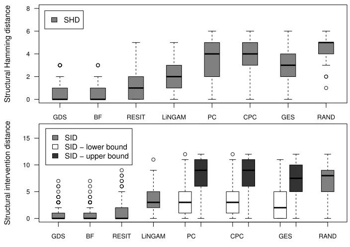
(modestly) sparse setting. For a linear and a nonlinear setting we report the average struc-tural Hamming distance (Acid and de Campos, 2003; Tsamardinos et al., 2006) to the true directed acyclic graph and to the true completed partially directed acyclic graph over 100 simulations. The structural Hamming distance (SHD) between two partially directed acyclic graphs counts how many edge types do not coincide. Estimating a non-edge or a directed edge instead of an undirected edge, for example, contributes an error of one to the overall distance. We also report analogous results for the structural intervention distance (SID),

which has recently been proposed (Peters and B¨uhlmann, 2013). Given the estimated graph

we can infer the intervention distributionp(Xj|do(Xi=xi)) by parent adjustment (1). We

call a pair of nodes (Xi, Xj)goodif the intervention distributionp(Xj|do(Xi=xi)) inferred

from the estimated DAG using (1) coincides with the intervention distribution inferred from

the correct DAG for all observational distributions L(X). The SID counts the number of

pairs that are not good. Some methods output a Markov equivalence class instead of a single DAG. Different DAGs within such a class lead to different intervention distribution and thus different SIDs. In that case, we therefore provide the smallest and largest SID attained by members within the Markov equivalence class. As the SHD, the SID is a purely structural measure that is independent of any distribution. The rationale behind the new measure is that a reversed edge in the estimated DAG leads to more false causal effects than an additional edge does. The SHD, however, weights both errors equally.

We compare the greedy DAG search (GDS), brute-force (BF), regression with subse-quent independence test (RESIT), linear non-Gaussian additive models (LINGAM), the PC

algorithm (PC) with partial correlation and significance level 0.01 and greedy equivalence

search (GES), see Sections 4.2.2, 4.2.1, 4.1, 2.3, 2.1 and 2.2, respectively. We also compare them with the conservative PC algorithm (CPC), suggested by Ramsey et al. (2006), and random guessing (RAND). The latter chooses a random DAG with edge inclusion proba-bility uniformly chosen between zero and one. Its estimate does not depend on the data.

5.1.1 Linear Structural Equation Models

We first consider a linear setting as in equation (4), where the coefficientsβjk are uniformly

chosen from [−2,−0.1]∪[0.1,2] and the noise variablesNj are independent and distributed

according toKj·sign(Mj)·|Mj|αj withMj

iid

∼ N(0,1),Kj iid

∼ U([0.1,0.5]) andαj

iid

∼ U([2,4]). The top box plot in Figure 3 compares the SHD of the estimated structure to the correct

DAG forp= 4 andn= 100. All methods make use of the linear structure of the data, e.g.,

search performs almost equally well, it does not encounter many local optima in this setting. The constraint-based methods and greedy equivalent search perform worse. Comparing SID leads to the same conclusion (Figure 3, bottom).

● ● ● ● ● ●

● ●●●

●

● ●

GDS BF RESIT LiNGAM PC CPC GES RAND

0 2 4 6 8

Str

uctur

al Hamming distance

SHD

● ●

● ● ● ● ●

● ● ●

● ● ● ● ● ● ●

●

● ● ● ● ● ●

● ●

● ● ● ● ● ●

● ● ●

● ● ● ● ●

●

● ●

GDS BF RESIT LiNGAM PC CPC GES RAND

0 5 10 15

Str

uctur

al inter

vention distance

SID

SID − lower bound SID − upper bound

Figure 3: Box plots of the SHD between the estimated structure (either DAG or CPDAG)

and the correct DAG forp= 4 andn= 100 for linear non-Gaussian SEMs (top).

The SID is computed between the correct DAG and the estimated DAG (bottom). Some methods estimate only the Markov equivalence class. We then compute the SID to the “best” and to the “worst” DAG within the equivalence class; therefore a lower and an upper bound are shown.

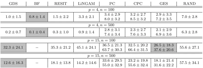
Tables 1 and 2 provide summaries for p∈ {4,15} and n∈ {100,500}. We additionally

show distances of the estimated CPDAGs to the true CPDAGs. Therefore, if methods output a DAG instead of a CPDAG, this DAG is transformed into the CPDAG of the

corresponding Markov equivalence class. For p= 4 andn= 500, GDS and brute force find

almost always the correct graph (86 and 90 out of 100). RESIT and LiNGAM still perform

much better than the PC methods and GES. For p= 15, the performance of RESIT (and

GES) in relation to the other methods seems to be better when evaluating SID compared to evaluating the SHD. This indicates that the pruning (and penalization of the number of edges) does not work perfectly. Especially for RESIT with high sample size and fixed significance level, making mistakes in phase 1 leads to many edges that cannot be removed

Table 1: Linear SEMs: SHD between the estimated structure and the correct DAG and SHD between the estimated CPDAG to the correct CPDAG; for both the average and the standard deviation over 100 experiments are shown (best averages are highlighted).

GDS BF RESIT LiNGAM PC CPC GES RAND

p= 4, n= 100

DAG 0.7±0.9 0.6±0.8 1.2±1.3 1.9±1.2 3.5±1.5 3.6±1.4 3.1±1.7 4.4±1.0 CPDAG 1.1±1.5 0.9±1.4 1.5±1.7 2.4±1.5 2.4±1.7 2.3±1.6 2.0±2.0 4.3±1.4

p= 4, n= 500

DAG 0.2±0.6 0.1±0.3 0.6±0.8 0.5±0.8 3.1±1.4 3.2±1.4 2.9±1.6 4.1±1.2 CPDAG 0.3±0.9 0.2±0.5 0.9±1.3 0.8±1.2 1.9±1.8 1.6±1.7 1.6±1.9 3.9±1.4

p= 15, n= 100

DAG 12.2±5.3 − 25.2±8.3 11.1±3.7 13.0±3.6 13.7±3.7 12.7±4.2 57.4±26.4 CPDAG 13.2±5.4 − 27.0±8.5 12.4±3.9 10.7±3.5 10.8±3.8 12.4±4.9 58.5±27.1

p= 15, n= 500

DAG 6.1±6.4 − 51.2±17.8 3.4±2.8 10.2±3.8 10.8±4.2 8.7±4.6 57.6±24.2 CPDAG 6.8±6.9 − 54.5±18.5 4.5±3.8 8.2±4.6 7.5±4.4 7.1±5.6 58.9±25.0

Table 2: Linear SEMs: SID to the correct DAG; the table shows average and standard deviation over 100 experiments.

GDS BF RESIT LiNGAM PC CPC GES RAND

p= 4, n= 100

1.0±1.5 0.8±1.4 1.5±2.2 3.3±2.1 3.4±2.9 3.2±2.7 2.9±3.3 7.0±2.8 8.0±3.2 8.5±3.2 7.2±3.5

p= 4, n= 500

0.2±0.7 0.1±0.4 0.3±1.0 0.9±1.4 2.8±3.1 2.3±2.7 2.1±2.9 6.3±2.8 7.4±3.4 7.6±3.3 6.9±3.6

p= 15, n= 100

− 35.3±21.2 45.1±24.1 36.5±21.3 32.5±20.2 26.5±18.3 55.6±27.1 32.3±24.1

63.7±30.3 66.4±31.5 37.6±20.6 p= 15, n= 500

− 18.1±13.8 14.2±14.6 33.6±29.5 23.2±19.8 18.1±21.4 57.5±34.1 12.6±16.3

55.0±32.9 55.6±32.4 31.6±22.2

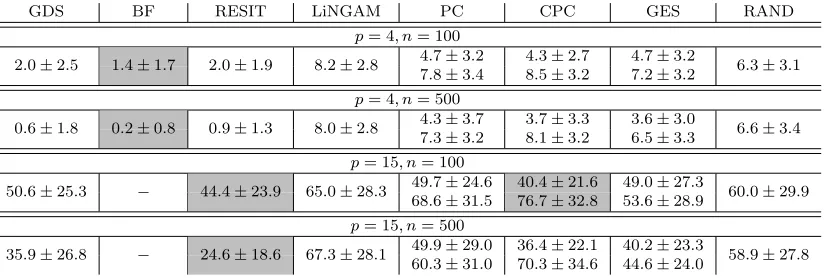
5.1.2 Nonlinear Structural Equation Models

We also sample data from nonlinear SEMs. We choose an additive structure as in equa-tion (8) and sample the funcequa-tions from a Gaussian process with bandwidth one. The noise

variables Nj are independent and normally distributed with a uniformly chosen variance.

Tables 3 and 4 show summaries for p ∈ {4,15} and n ∈ {100,500}. We cannot run the

brute-force method on data sets with p = 15. For p = 4, we have a similar situation as

in Figure 3 with GDS and the BF method outperforming all others (RESIT performing a

bit worse). Remarkably, for p = 15 and n = 100, a lot of the methods do not perform

Table 3: Nonlinear SEMs: SHD between the estimated structure and the correct DAG and SHD between the estimated CPDAG to the correct CPDAG; for both the average and the standard deviation over 100 experiments are shown.

GDS BF RESIT LiNGAM PC CPC GES RAND

p= 4, n= 100

DAG 1.5±1.4 1.0±1.0 1.7±1.3 3.5±1.2 3.5±1.5 3.8±1.4 3.5±1.3 4.0±1.3 CPDAG 1.7±1.7 1.2±1.4 2.0±1.6 3.0±1.4 2.9±1.5 2.7±1.4 3.4±1.7 3.9±1.4

p= 4, n= 500

DAG 0.5±0.9 0.3±0.5 0.8±0.9 3.7±1.2 3.5±1.5 3.8±1.5 3.3±1.5 4.1±1.2 CPDAG 0.6±1.1 0.6±1.0 1.0±1.3 3.0±1.7 3.1±1.9 2.8±1.8 3.4±1.9 3.8±1.6

p= 15, n= 100

DAG 14.3±4.9 − 15.4±5.7 15.4±3.6 14.2±3.5 15.5±3.6 24.8±6.3 56.8±24.1 CPDAG 15.1±5.4 − 16.5±5.9 15.3±4.0 13.3±3.6 13.3±4.0 26.4±6.5 58.0±24.7

p= 15, n= 500

DAG 13.0±8.4 − 10.1±5.7 21.4±6.9 13.9±4.5 15.1±4.8 26.8±8.5 56.1±26.8 CPDAG 14.2±9.2 − 11.3±6.3 21.1±7.3 13.7±4.9 13.4±5.1 28.6±8.8 57.0±27.3

Table 4: Nonlinear SEMs: SID to the correct DAG; the table shows average and standard deviation over 100 experiments.

GDS BF RESIT LiNGAM PC CPC GES RAND

p= 4, n= 100

2.0±2.5 1.4±1.7 2.0±1.9 8.2±2.8 4.7±3.2 4.3±2.7 4.7±3.2 6.3±3.1 7.8±3.4 8.5±3.2 7.2±3.2

p= 4, n= 500

0.6±1.8 0.2±0.8 0.9±1.3 8.0±2.8 4.3±3.7 3.7±3.3 3.6±3.0 6.6±3.4 7.3±3.2 8.1±3.2 6.5±3.3

p= 15, n= 100

50.6±25.3 − 44.4±23.9 65.0±28.3 49.7±24.6 40.4±21.6 49.0±27.3 60.0±29.9 68.6±31.5 76.7±32.8 53.6±28.9

p= 15, n= 500

35.9±26.8 − 24.6±18.6 67.3±28.1 49.9±29.0 36.4±22.1 40.2±23.3 58.9±27.8 60.3±31.0 70.3±34.6 44.6±24.0

means that some DAGs within the equivalence class perform much better than others. (The methods do not propose any particular DAG, they treat all DAGs within the class equally.)

Figure 4 shows box plots of SHD and SID for the special case p = 15 and n = 500.

This time, RESIT perform slightly better than all other methods. It makes use of the nonlinearity of the structural equations. Again, the high SHD for GES indicates that the estimate probably contains too many edges (since its SID is better than the one for the PC methods).

In conclusion, forp= 4, the brute force method works best for both linear and nonlinear

data. Roughly speaking, for p = 15, LiNGAM and GDS work best in the linear