Local Causal and Markov Blanket Induction for Causal Discovery
and Feature Selection for Classification
Part I: Algorithms and Empirical Evaluation
Constantin F. Aliferis [email protected]
Center of Health Informatics and Bioinformatics Department of Pathology
New York University New York, NY 10016, USA
Alexander Statnikov [email protected]
Center of Health Informatics and Bioinformatics Department of Medicine
New York University New York, NY 10016, USA
Ioannis Tsamardinos [email protected]
Computer Science Department, University of Crete
Institute of Computer Science, Foundation for Research and Technology, Hellas Heraklion, Crete, GR-714 09, Greece
Subramani Mani [email protected]
Discovery Systems Laboratory Department of Biomedical Informatics Vanderbilt University
Nashville, TN 37232, USA
Xenofon D. Koutsoukos [email protected]
Department of Electrical Engineering and Computer Science Vanderbilt University
Nashville, TN 37212, USA
Editor: Marina Meila
Abstract
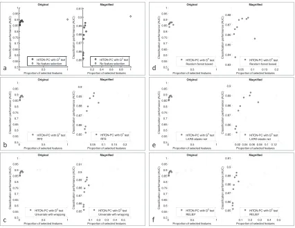
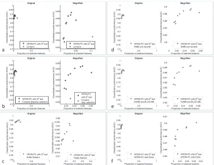
We present an algorithmic framework for learning local causal structure around target variables of interest in the form of direct causes/effects and Markov blankets applicable to very large data sets with relatively small samples. The selected feature sets can be used for causal discovery and clas-sification. The framework (Generalized Local Learning, or GLL) can be instantiated in numerous ways, giving rise to both existing state-of-the-art as well as novel algorithms. The resulting algo-rithms are sound under well-defined sufficient conditions. In a first set of experiments we evaluate several algorithms derived from this framework in terms of predictivity and feature set parsimony and compare to other local causal discovery methods and to state-of-the-art non-causal feature se-lection methods using real data. A second set of experimental evaluations compares the algorithms in terms of ability to induce local causal neighborhoods using simulated and resimulated data and examines the relation of predictivity with causal induction performance.
distribu-tions, types of classifiers, and loss functions) exhibit strong feature set parsimony, high predictivity and local causal interpretability. Although non-causal feature selection methods are often used in practice to shed light on causal relationships, we find that they cannot be interpreted causally even when they achieve excellent predictivity. Therefore we conclude that only local causal techniques should be used when insight into causal structure is sought.
In a companion paper we examine in depth the behavior of GLL algorithms, provide extensions, and show how local techniques can be used for scalable and accurate global causal graph learning.
Keywords: local causal discovery, Markov blanket induction, feature selection, classification, causal structure learning, learning of Bayesian networks
1. Introduction
This paper addresses the problem of how to learn local causal structure around a target variable of interest using observational data. We focus on two specific types of local discovery: (a) identifica-tion of variables that are direct causes or direct effects of the target, and (b) discovery of Markov blankets. A Markov Blanket of a variable T is a minimal variable subset conditioned on which all other variables are probabilistically independent of T .
Discovery of local causal relationships is significant because it plays a central role in causal discovery and classification, because of its scalability benefits, and because by naturally bridging causation with predictivity, it provides significant benefits in feature selection for classification. More specifically, solving the local causal induction problem helps understanding how natural and artificial systems work; it helps identify what interventions to pursue in order for these systems to exhibit desired behaviors; under certain assumptions, it provides minimal feature sets required for classification of a chosen response variable with maximum predictivity; and finally local causal discovery can form the basis of efficient algorithms for learning the global causal structure of all variables in the data.
The paper is organized as follows: Section 2 provides necessary background material. The section summarizes related prior work in feature selection and causal discovery; reviews recent results that connect causality with predictivity; explains the central role of local causal discovery for achieving scalable global causal induction; reviews prior methods for local causal and Markov blanket discovery and published applications; finally it introduces the open problems that are the focus of the present report. Section 3 provides formal concepts and definitions used in the paper. Section 4 provides a general algorithmic framework, Generalized Local Learning (GLL), which can be instantiated in many different ways yielding sound algorithms for local causal discovery and fea-ture selection. Section 5 evaluates a multitude of algorithmic instantiations and parameterizations from GLL and compares them to state-of-the-art local causal discovery and feature selection meth-ods in terms of classification performance, feature set parsimony, and execution time in many real data sets. Section 6 evaluates and compares new and state-of-the-art algorithms in terms of ability to induce correct local neighborhoods using simulated data from known networks and resimulated data from real-life data sets. Section 7 discusses the experimental findings and their significance.
empirically and theoretically, introduces algorithmic extensions, and connects local to global causal graph learning (Aliferis et al., 2010). An online supplement to the present work is available at
http://www.nyuinformatics.org/downloads/supplements/JMLR2009/index.html. In
ad-dition to supplementary tables and figures, the supplement provides all software and data needed to reproduce the analyses of the present paper.
2. Background
In the present section we provide a brief review of feature selection and causal discovery research, summarize theoretical results motivating this work, present methods to speed-up scalability of dis-covery, give desiderata for local algorithms, review prior methods for Markov blanket and local neighborhood induction, and finally discuss open problems and focus of this paper.
2.1 Brief Review of Feature Selection and Causal Discovery Research
Variable selection for predictive modeling (also called feature selection) has received considerable attention during the last three decades both in statistics and in machine learning (Guyon and Elisse-eff, 2003; Kohavi and John, 1997). Intuitively, variable selection for prediction aims to select only a subset of variables for constructing a diagnostic or predictive model for a given classification or regression task. The reasons to perform variable selection include (a) improving the model predic-tivity and addressing the curse-of-dimensionality, (b) reducing the cost of observing, storing, and using the predictive variables, and finally, (c) gaining an understanding of the underlying process that generates the data. The problem of variable selection is more pressing than ever, due to the re-cent emergence of extremely large data sets, sometimes involving tens to hundreds of thousands of variables and exhibiting a very small sample-to-variable ratio. Such data sets are common in gene expression array studies, proteomics, computational biology, text categorization, information re-trieval, image classification, business data analytics, consumer profile analysis, temporal modeling, and other domains and data-mining applications.
There are many different ways to define the variable selection problem depending on the needs of the analysis. Often however, the feature selection problem for classification/prediction is defined as identifying the minimum-size subset of variables that exhibit the maximal predictive performance (Guyon and Elisseeff, 2003). Variable selection methods can be broadly categorized into wrappers (i.e., heuristic search in the space of all possible variable subsets using a classifier of choice to assess each subset’s predictive information), or filters (i.e., not using the classifier per se to select features, but instead applying statistical criteria to first select features and then build the classifier with the best features). In addition, there exist learners that perform embedded variable selection, that is, that attempt to simultaneously maximize classification performance while minimizing the number of variables used. For example, shrinkage regression methods introduce a bias into the parameter estimation regression procedure that imposes a penalty on the size of the parameters. The parameters that are close to zero are essentially filtered-out from the predictive model.
A variety of embedded variable selection methods have been recently introduced. These meth-ods are linked to a statement of the classification or regression problem as an optimization problem with specified loss and penalty functions. These techniques usually fall into a few broad classes:
One class of methods uses the
L
2-norm penalty (also known as ridge penalty), for example, there-cursive feature elimination (RFE) method is based on the
L
2-norm formulation of SVMpenalty (also known as lasso penalty), for example, feature selection via solution of the
L
1-normformulation of SVM classification problem (Zhu et al., 2004; Fung and Mangasarian, 2004) and penalized least squares with lasso penalty on the regression coefficients (Tibshirani, 1996). A third
set of methods is based on convex combinations of the
L
1- andL
2-norm penalties, for example,feature selection using the doubly SVM formulation (Wang et al., 2006) and penalized least squares
with elastic net penalty (Zou and Hastie, 2005). A fourth set uses the
L
0-norm penalty, for example,feature selection via approximate solution of the
L
0-norm formulation of SVM classificationprob-lem (Weston et al., 2003). Finally other methods use other penalties, for example, smoothly clipped absolute deviation penalty (Fan and Li, 2001).
Despite the recent emphasis on mathematically sophisticated methods such as the ones men-tioned, the majority of feature selection methods in the literature and in practice are heuristic in nature in the sense that in most cases it is unknown what consists an optimal feature selection solu-tion independently of the class of models fitted, and under which condisolu-tions an algorithm will output such an optimal solution.
Typical variable selection approaches also include forward, backward, forward-backward, local and stochastic search wrappers (Guyon and Elisseeff, 2003; Kohavi and John, 1997; Caruana and Freitag, 1994). The most common family of filter algorithms ranks the variables according to a score and then selects for inclusion the top k variables (Guyon and Elisseeff, 2003). The score of each variable is often the univariate (pairwise) association with the outcome variable T for different
measures of associations such as the signal-to-noise ratio, the G2 statistic and others.
Information-theoretic (estimated mutual information) scores and multivariate scores, such as the weights re-ceived by a Support Vector Machine, have also been suggested (Guyon and Elisseeff, 2003; Guyon et al., 2002). Excellent recent reviews of feature selection can be found in Guyon et al. (2006a), Guyon and Elisseeff (2003) and Liu and Motoda (1998).
An emerging successful but also principled filtering approach in variable selection, and the one largely followed in this paper, is based on identifying the Markov blanket of the response (“target”)
variable T . The Markov blanket of T (denoted as MB(T)) is defined as a minimal set conditioned
growth of biomedical and other data cannot be made in any reasonable amount of time using solely the classical experimental approach where a single gene, protein, treatment, or intervention is at-tempted each time, since the space of needed experiments is immense. It is clear that computational methods are needed to catalyze the discovery process.
Fortunately, relatively recently (1980’s), it was shown that it is possible to soundly infer causal relations from observational data in many practical cases (Spirtes et al., 2000; Pearl, 2000; Glymour and Cooper, 1999; Pearl, 1988). Since then, algorithms that infer such causal relations have been developed that can greatly reduce the number of experiments required to discover the causal struc-ture. Several empirical studies have verified their applicability (Tsamardinos et al., 2003b; Spirtes et al., 2000; Glymour and Cooper, 1999; Aliferis and Cooper, 1994).
One of the most common methods to model and induce causal relations is by learning causal Bayesian networks (Neapolitan, 2004; Spirtes et al., 2000; Pearl, 2000). A special, important and quite broad class of such networks is the family of faithful networks intuitively defined as those whose probabilistic properties, and specifically the dependencies and independencies, are a direct function of their structure (Spirtes et al., 2000). Cooper and Herskovits were the first to devise a score measuring the fit of a network structure to the data based on Bayesian statistics, and used it to learn the highest score network structure (Cooper and Herskovits, 1992). Heckerman and his colleagues studied theoretically the properties of the various scoring metrics as they pertain to causal discovery (Glymour and Cooper, 1999; Heckerman, 1995; Heckerman et al., 1995). Heckerman also recently showed that Bayesian-scoring methods also assume (implicitly) faithfulness, see Chapter 4 of Glymour and Cooper (1999). Another prototypical method for learning causal relationships by inducing causal Bayesian networks is the constraint-based approach as exemplified in the PC algorithm by Spirtes et al. (2000). The PC induces causal relations by assuming faithfulness and by performing tests of independence. A network with a structure consistent with the results of the tests of independence is returned. Several other methods for learning networks have been devised subsequently (Chickering, 2003; Moore and Wong, 2003; Cheng et al., 2002a; Friedman et al., 1999b).
There may be many different networks that fit the data equally well, even in the sample limit, and that exhibit the same dependencies and independencies and are thus statistically equivalent. These networks belong to the same Markov equivalence class of causal graphs and contain the same causal edges but may disagree on the direction of some of them, that is, whether A causes B or vice-versa (Chickering, 2002; Spirtes et al., 2000). An essential graph is a graph where the directed edges represent the causal relations on which all equivalent networks agree upon their directionality and all the remaining edges are undirected. Causal discovery by employing causal Bayesian networks is based on the following principles. The PC (Spirtes et al., 2000), Greedy Equivalence Search (Chickering, 2003) and other prototypical or state-of-the-art Bayesian network-learning algorithms provide theoretical guarantees, that under certain conditions such as faithfulness they will converge to a network that is statistically indistinguishable from the true, causal, data-generating network, if there is such. Thus, if the conditions hold the existence of all and the direction of some of the causal relations can be induced by these methods and graphically identified in the essential graph of the learnt network.
presence of hidden confounding variables and selection bias, have also been designed (see Spirtes et al. 2000 and Chapter 6 of Glymour and Cooper 1999).
As it was mentioned above, using observational data alone (even a sample of an infinite size), one can infer only a Markov equivalence class of causal graphs, which may be inadequate for causal discovery. For example, it is not possible to distinguish with observational data any of these
two graphs that belong to the same Markov equivalence class: X →Y and X ←Y . However,
experimental data can distinguish between these graphs. For example, if we manipulate X and see
no change in the distribution of Y , we can conclude that the data-generative graph is not X →Y .
This principle is exploited by active learning algorithms. Generally speaking, causal discovery with active learning can be described as follows: learn an approximation of a causal network structure from available data (which is initially only observational data), select and perform an experiment that maximizes some utility function, augment data and possibly current best causal network with the result of experiment, and repeat the above steps until some termination criterion is met.
Cooper and Yoo (1999) proposed a Bayesian scoring metric that can incorporate both observa-tional and experimental data. Using a similar metric (Tong and Koller, 2001) designed an algorithm to select experiments that reduce the entropy of probability of alternative edge orientations. A simi-lar but more general algorithm has been proposed in Murphy (2001) where the expected information gain of a new experiment is calculated and the experiment with the largest information gain is se-lected. Both above methods were designed for discrete data distributions. Pournara and Wernisch (2004) proposed another active learning algorithm that uses a loss function defined in terms of the size of transition sequence equivalence class of networks (Tian and Pearl, 2001) and can handle continuous data. Meganck et al. (2006) have introduced an active learning algorithm that is based on a general decision theoretic framework that allows to assign costs to each experiment and each measurement. It is also worthwhile to mention the GEEVE system of Yoo and Cooper (2004) that recommends which experiments to perform to discover gene-regulation pathway. This instance of causal active learning allows to incorporate preferences of the experimenter. Recent work has also provided theoretical bounds and related algorithms to minimize the number of experiments needed to infer causal structure (Eberhardt et al., 2006, 2005).
2.2 Synopsis of Theoretical Results Motivating Present Research
A key question that has been investigated in the feature selection literature is which family of meth-ods is more advantageous: filters or wrappers. A second one is what are the “relevant” features? The latter question presumably is important because “relevant” features should be important for dis-covery and so several definitions appeared defining relevancy (Guyon and Elisseeff, 2003; Kohavi and John, 1997). Finally, how can we design optimal and efficient feature selection algorithms? Fundamental theoretical results connecting Markov blanket induction for feature selection and local causal discovery to standard notions of relevance were given in Tsamardinos and Aliferis (2003). The latter paper provides a technical account and together with Spirtes et al. (2000), Pearl (2000), Kohavi and John (1997) and Pearl (1988) they constitute the core theoretical framework underpin-ning the present work. Here we provide a very concise description of the results in Tsamardinos and Aliferis (2003) since they partially answer these questions and pave the way to principled feature selection:
selection problem. The quest for a universally applicable notion of relevancy for prediction is futile.
2. Wrappers are subject to the No-Free Lunch Theorem for optimization: averaged out on all possible problems any wrapper algorithm will do as well as a random search in the space of feature subsets. Therefore, there cannot be a wrapper that is a priori more efficient than any other (i.e., without taking into account the learner and model-performance metric). The quest for a universally efficient wrapper is futile as well.
3. Any filter algorithm can be viewed as the implementation of a definition of relevancy. Because of #1, there is no filter algorithm that is universally optimal, independently of the learner and model-performance metric.
4. Because of #2, wrappers cannot guarantee universal efficiency and because of #3, filters can-not guarantee universal optimality and in that respect, neither approach is superior to the other.
5. Under the conditions that (i) the learner that constructs the classification model can actually
learn the distribution P(T|MB(T))and (ii) that the loss function is such that perfect estimation
of the probability distribution of T is required with the smallest number of variables, the Markov blanket of T is the optimal solution to the feature selection problem.
6. Sound Markov blanket induction algorithms exist for faithful distributions.
7. In faithful distributions and under the conditions of #5, the strongly/weakly/irrelevant taxon-omy of variables (Kohavi and John, 1997) can be mapped naturally to causal graph properties. Informally stated, strongly relevant features were defined by Kohavi and John (1997) to be features that contain information about the target not found in other variables; weakly relevant features are informative but redundant; irrelevant features are not informative (for formal defi-nitions see Section 3). Under the causal interpretation of this taxonomy of relevancy, strongly relevant features are the members of the Markov blanket of the target variable, weakly rele-vant features are all variables with an undirected path to T which are not themselves members
of MB(T), and irrelevant features are variables with no undirected path to the target.
8. Since in faithful distributions the MB(T)contains the direct causes and direct effects of T , and
since state-of-the-art MB(T)algorithms output the spouses separately from the direct causes
and direct effects, inducing the MB(T)not only solves the feature selection problem but also
a form of local causal discovery problem.
Figure 1 provides a summary of the connection between causal structure and predictivity.
Ê
Ê
E C
T
F D
G
I
A B
H K
J
L
Relationship between causal structure and predictivity in faithful distributions.
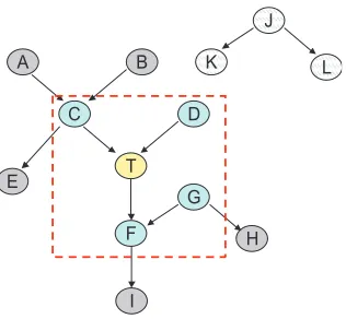
Figure 1: Relationship between causal structure and predictivity in faithful distributions. Cyan variables are members of Markov blanket of T . They are depicted inside the red dotted square (i.e., variables that have undirected path to target T and that are predictive of T given the remaining variables which makes them strongly relevant). Markov blanket variables include direct causes of T
(C,D), direct effects(F), and “spouses” of T (i.e., direct causes of the direct effects of T )(G). Grey
variables are non-members of Markov blanket of T that have undirected path to T . They are not predictive of T given the remaining variables but they are predictive given a subset of the remaining variables (which makes them weakly relevant). Light-gray variables are variables that do not have an undirected path to T . They are not predictive of T given any subset of the remaining variables, thus they are irrelevant.
correct causal neighborhood and are not minimal, that is, do not solve the feature selection problem) even in the large sample limit.
The above theoretical results also suggest that one should not attempt to define and identify the relevant features for prediction, when discovery is the goal of the analysis. Instead, we argue that a set of features with well-defined causal semantics should be identified instead: for example, the
MB(T), the set of direct causes and direct effects of T , the set of all (direct and indirect) causes of
T , and so on.
We will investigate limitations of prominent non-causal feature selection algorithms in the com-panion paper (Aliferis et al., 2010).
2.3 Methods to Speed-up Discovery: Local Discovery as a Critical Tool for Scalability
With the advent of massive data sets in biology, medicine, information retrieval, the WWW, finance, economics, and so on, scalability has become a critical requirement for practical algorithms. In early 2000’s predictions about the feasibility of causal discovery in high-dimensional data were bleak (Silverstein et al., 2000). A variety of methods to scale up causal discovery have been devised to address the problem:
1. Learn the full graph but focus on special types of distributions;
2. Exploit domain knowledge to speed-up learning;
3. Abandon the effort to learn the full causal graph and instead develop methods that find a portion of the true arcs (not specific to some target variable);
4. Abandon the effort to learn the full causal graph and instead develop methods that learn the local neighborhood of a specific target variable directly;
5. Abandon the effort to learn the fully oriented causal graph and instead develop methods that learn the unoriented graph;
6. Induce constrains of the possible relationships among variables and then learn the full causal graph.
Techniques #1 and #2 were introduced in Chow and Liu (1968) for learning tree-like graphs and Na¨ıve-Bayes graphs (Duda and Hart, 1973), while modern versions are exemplified in (i) TAN/BAN classifiers that relax the Na¨ıve-Bayes structure (Cheng and Greiner, 2001, 1999; Friedman et al., 1997), (ii) efficient complete model averaging of Na¨ıve-Bayes classifiers (Dash and Cooper, 2002), and (iii) algorithm TPDA which restricts the class of distributions so that learning becomes from
worst-case intractable to solvable in 4th degree polynomial time to the number of variables (and
quadratic if prior knowledge about the ordering of variables is known) (Cheng et al., 2002a). Tech-nique #3 was introduced by Cooper (1997) and replaced learning the complete graph by learning only a small portion of the edges (not pre-specified by the user but determined by the discovery
method). Techniques #4−6 pertain to local learning: Technique #4 seeks to learn the complete
causal neighbourhood around a target variable provided by the user (Aliferis et al., 2003a; Tsamardi-nos et al., 2003b). We emphasize that local learning (technique #4) is not the same as technique #3 (incomplete learning) although inventors of incomplete methods often call them ‘local’. Technique #5 abandons directionality and learns only a fully connected but undirected graph by using local learning methods (Tsamardinos et al., 2006; Brown et al., 2005). Often post-processing with ad-ditional algorithms can provide directionality. The latter can also be obtained by domain-specific criteria or experimentation. Finally, technique #6 uses local learning to restrict the search space for full-graph induction algorithms (Tsamardinos et al., 2006; Aliferis and Tsamardinos, 2002b).
B A
E
T
H Q L
M N P O C D I J K F G R S U V W X Y Z B A E T
H Q L
M N P O C D I J K F G R S U V W X Y Z A E T
H Q L
M N P O C D I J K F G R S U V W X Y Z B B A E T
H Q L
M N P O C D I J K F G R S U V W X Y Z
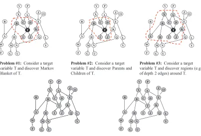
Problem #1: Consider a target
variable T and discover Markov Blanket of T.
Problem #2: Consider a target
variable T and discover Parents and Children of T.
Problem #3: Consider a target
variable T and discover regions (e.g., of depth 2 edges) around T.
Problem #5: Discover undirected graph.
A E
T
H Q L
M N P O C D I J K F G R S U V W X Y Z B A E T
H Q L
M N P O C D I J K F G R S U V W X Y Z B
Problem #4: Discover directed graph.
Figure 2: Five types of causal discovery from local (types 1, 2), to global (4, 5) and intermediate (3). Specialized algorithms that solve type 2 (local causes and effects) can become building blocks for relatively efficiently solving all other types of causal discovery as well (see text for details).
2.4 Desiderata for Local Algorithms, Brief Review of Prior Methods for Markov Blanket and Local Neighborhood Induction
An ideal local learning algorithm should have three characteristics: (a) well-defined properties, es-pecially broadly applicable conditions that guarantee correctness, (b) good performance in practical distributions and corresponding data sets, including ones with small sample and many features, and finally (c) scalability in terms of running time. We briefly review progress made in the field toward these goals.
Firm theoretical foundations of Bayesian networks were laid down by Pearl and his co-authors (Pearl, 1988). Furthermore, all local learning methods exploit either the constraint-based frame-work for causal discovery developed by Spirtes, Glymour, Schienes, Pearl, and Verma and their co-authors (Spirtes et al., 2000; Pearl, 2000; Pearl and Verma, 1991) or the Bayesian search-and-score Bayesian network learning framework introduced by Cooper and Herskovits (1992). The relevant key contributions were covered in Section 2.1 and will not be repeated here.
Markov blanket from data and tested the algorithm in simulated, real text, and other types of data from the UCI repository (Koller and Sahami, 1996). In 1997 Cooper and colleagues introduced and applied the heuristic method K2MB for finding the Markov blanket of a target variable in the task of predicting pneumonia mortality (Cooper, 1997). In 1997 Cooper introduced an incomplete method for causal discovery (Cooper et al., 1997). The algorithm was able to circumvent lack of scalability of global methods by returning a subset of arcs from the full network. To avoid notational confusion we point out that the algorithm was termed LCD (local causal discovery) despite being an incomplete rather than local algorithm as local algorithms are defined in the present paper (i.e., focused on some user-specified target variable or localized region of the network). A revision of the algorithm termed LCD2 was presented in Mani and Cooper (1999).
In 1999 Margaritis and Thrun introduced the GS algorithm with the intent to induce the Markov blanket for the purpose of speeding up global network learning (i.e., not for feature selection) (Mar-garitis and Thrun, 1999). GS was the first published sound Markov blanket induction algorithm. The weak heuristic used by GS combined with the need to condition on at least as many variables simultaneously as the Markov blanket size makes it impractical for many typical data sets since the required sample grows exponentially to the size of the Markov blanket. This in turn forces the algo-rithm to stop its execution prematurely (before it identifies the complete Markov blanket) because it cannot grow the conditioning set while performing reliable tests of independence. Evaluations of GS by its inventors were performed in data sets with a few dozen variables leaving the potential of scalability largely unexplored.
In 2001 Cheng et al. applied the TPDA algorithm (a global BN learner) (Cheng et al., 2002a) to learn the Markov blanket of the target variable in the Thrombin data set in order to solve a prediction problem of drug effectiveness on the basis of molecular characteristics (Cheng et al., 2002b). Because TPDA could not be run with more than a few hundred variables efficiently, they pre-selected 200 variables (out of 139,351 total) using univariate filtering. Although this procedure in general will not find the true Markov blanket (because otherwise-unconnected with the target spouses can be missed, many true parents and children may not be in the first 200 variables, and many non-Markov blanket members cannot be eliminated), the resulting classifier performed very well winning the 2001 KDD Cup competition.
Friedman et al. proposed a simple Bootstrap procedure for determining membership in the Markov blanket for small sample situations (Friedman et al., 1999a). The Markov blanket in this method is to be extracted from the full Bayesian network learned by the SCA (Sparse Candidate Algorithm) learner (Friedman et al., 1999b).
In 2002 and 2003 Tsamardinos, Aliferis, et al. presented a modified version of GS, termed IAMB and several variants of the latter that through use of a better inclusion heuristic than GS and optional post-processing of the tentative and final output of the local algorithm with global learners would achieve true scalability to data sets with many thousands of variables and applicability in modest (but not very small) samples (Tsamardinos et al., 2003a; Aliferis et al., 2002). IAMB and several variants were tested both in the high-dimensional Thrombin data set (Aliferis et al., 2002) and in data sets simulated from both existing and random Bayesian networks (Tsamardinos et al., 2003a). The former study found that IAMB scales to high-dimensional data sets. The latter study compared IAMB and its variants to GS, Koller-Sahami, and PC and concluded that IAMB variants on average perform best in the data sets tested.
(Tsamardi-nos and Aliferis, 2003). They also provided theoretical results about the strengths and weaknesses of filter versus wrapper algorithms, the impossibility of a universal definition of relevance, and the optimality of Markov blanket as a solution to the feature selection problem in formal terms. These results were summarized in Section 2.2.
The extension of Sparse Candidate Algorithm to create a local-to-global learning strategy was first introduced in Aliferis and Tsamardinos (2002b) and led to the MMHC algorithm introduced and evaluated in Tsamardinos et al. (2006). MMHC was shown in Tsamardinos et al. (2006) to achieve best-of-class performance in quality and scalability compared to most state-of-the-art global network learning algorithms.
In 2002 Aliferis et al. also introduced parallel and distributed versions of the IAMB family of algorithms (Aliferis et al., 2002). These serve as the precursor of the parallel and distributed local neighborhood learning method presented in the companion paper (Aliferis et al., 2010). The precursor of the GLL framework was also introduced by Aliferis and Tsamardinos in 2002 for the explicit purpose of reducing the sample size requirements of IAMB-style algorithms (Aliferis and Tsamardinos, 2002a).
In 2003 Aliferis et al. introduced algorithm HITON1 Aliferis et al., and Tsamardinos et al.
introduced algorithms MMPC and MMMB (Aliferis et al., 2003a; Tsamardinos et al., 2003b). These are the first concrete algorithms that would find sets of direct causes or direct effects and Markov blankets in a scalable and efficient manner. HITON was tested in 5 biomedical data sets spanning clinical, text, genomic, structural and proteomic data and compared against several feature selection methods with excellent results in parsimony and classification accuracy (Aliferis et al., 2003a). MMPC was tested in data simulated from human-derived Bayesian networks with excellent results in quality and scalability. MMMB was tested in the same data sets and compared to prior algorithms such as Koller-Sahami algorithm and IAMB variants with superior results in the quality of Markov blankets. These benchmarking and comparative evaluation experiments provided evidence that the local learning approach held not only theoretical but also practical potential.
HITON-PC, HITON-MB, MMPC, and MMMB algorithms lacked so-called “symmetry correc-tion” (Tsamardinos et al., 2006), however HITON used a wrapping post-processing that at least in principle removed this type of false positives. The symmetry correction was introduced in 2005 and 2006 by Tsamardinos et al. in the context of the introduction of MMHC (Tsamardinos et al., 2006, 2005). Pe˜na et al. also published work pointing to the need for a symmetry correction in MMPC (Pe˜na et al., 2005b).
HITON was applied in 2005 to understand physician decisions and guideline compliance in the diagnosis of melanomas (Sboner and Aliferis, 2005). HITON has been applied for the discovery of biomarkers in human cancer data using microarrays and mass spectrometry and is also imple-mented in the GEMS and FAST-AIMS systems for the automated analysis of microarray and mass spectrometry data respectively (Statnikov et al., 2005b; Fananapazir et al., 2005). In a recent ex-tensive comparison of biomarker selection algorithms (Aliferis et al., 2006a,b) it was found that HITON outperforms 16 state-of-the-art representatives from all major biomarker algorithmic fam-ilies in terms of combined classification performance and feature set parsimony. This evaluation used 9 human cancer data sets (gene expression microarray and mass spectrometry) in 10 diagnos-tic and outcome (i.e., survival) prediction classification tasks. In addition to the above real data, resimulation was also used to create two gold standard network structures, one re-engineered from
human lung cancer data and one from yeast data. Several applications of HITON in text categoriza-tion have been published where the algorithm was used to understand complex “black box” SVM models and convert complex models to Boolean queries usable by Boolean interfaces of Medline (Aphinyanaphongs and Aliferis, 2004), to examine the consistency of editorial policies in published journals (Aphinyanaphongs et al., 2006), and to predict drug-drug interactions (Duda et al., 2005). HITON was also compared with excellent results to manual and machine feature selection in the domain of early graft failure in patients with liver transplantations (Hoot et al., 2005).
In 2003 Frey et al. explored the idea of using decision tree induction to indirectly approximate the Markov blanket (Frey et al., 2003). They produced promising results, however a main problem with the method was that it requires a threshold parameter that cannot be optimized easily. Further-more, as we show in the companion paper (Aliferis et al., 2010) decision tree induction is subject to synthesis and does not select only the Markov blanket members.
In 2004 Mani et al. introduced BLCD-MB, which resembles IAMB but using a Bayesian scoring metric rather than conditional independence testing (Mani and Cooper, 2004). The algorithm was applied with promising results in infant mortality data (Mani and Cooper, 2004).
A method for learning regions around target variables by recursive application of MMPC or other local learning methods was introduced in Tsamardinos et al. (2003c). Pe˜na et al. applied interleaved MMPC for learning regions in the domain of bioinformatics (Pe˜na et al., 2005a).
In 2006 Gevaert et al. applied K2MB for the purpose of learning classifiers that could be used for prognosis of breast cancer from microarray and clinical data (Gevaert et al., 2006) . Univariate filtering was used to select 232 genes before applying K2MB.
Other recent efforts in learning Markov blankets include the following algorithms: PCX, which post-processes the output of PC (Bai et al., 2004); KIAMB, which addresses some violations of faithfulness using a stochastic extension to IAMB (Pe˜na et al., 2007); FAST-IAMB, which speeds up IAMB (Yaramakala and Margaritis, 2005); and MBFS, which is a PC-style algorithm that returns a graph over Markov blanket members (Ramsey, 2006).
2.5 Open Problems and Focus of Paper
The focus of the present paper is to describe state-of-the-art algorithms for inducing direct causes and effects of a response variable or its Markov blanket using a novel cohesive framework that can help in the analysis, understanding, improvement, application (including configuration / parameter-ization) and dissemination of the algorithms. We furthermore study comparative performance in terms of predictivity and parsimony of state-of-the-art local causal algorithms; we compare them to non-causal algorithms in real and simulated data sets using the same criteria; and show how novel algorithms can be obtained. A second major hypothesis (and set of experiments in the present pa-per) is that non-causal feature selection methods may yield predictively optimal feature sets while from a causal perspective their output is unreliable. Testing this hypothesis has tremendous implica-tions in many areas (e.g., analysis of biomedical molecular data) where highly predictive variables (biomarkers) of phenotype (e.g., disease or clinical outcome) are often interpreted as being causally implicated for the phenotype and great resources are invested in pursuing these markers for new drug development and other research.
behavior as well as several extensions including algorithms for learning the full causal graph using a divide-and-conquer local learning approach.
3. Notation and Definitions
In the present paper we use Bayesian networks as the language in which to represent data generating processes and causal relationships. We thus first formally define causal Bayesian networks. Recall that in a directed acyclic graph (DAG), a node A is the parent of B (B is the child of A) if there is a direct edge from A to B, A is the ancestor of B (B is the descendant of A) if there is a direct path from A to B. “Nodes”, “features”, and “variables” will be used interchangeably.
3.1 Notation
We will denote variables with uppercase letters X,Y,Z, values with lowercase letters, x,y,z, and sets
of variables or values with boldface uppercase or lowercase respectively. A “target” (i.e., response) variable is denoted as T unless stated otherwise.
Definition 1 Conditional Independence. Two variables X and Y are conditionally independent givenZ, denoted as I(X,Y|Z), iff P(X =x,Y =y|Z=z) =P(X =x|Z=z)P(Y =y|Z=z), for
all values x,y,zof X,Y,Zrespectively, such that P(Z=z)>0.
Definition 2 Bayesian networkhV,G,Ji. LetV be a set of variables and J be a joint probability
distribution over all possible instantiations ofV. Let G be a directed acyclic graph (DAG)such
that all nodes of G correspond one-to-one to members ofV. We require that for every node A∈V,
A is probabilistically independent of all non-descendants of A, given the parents of A (i.e., Markov
Condition holds). Then we call the triplethV,G,Jia Bayesian network (abbreviated as “BN”), or
equivalently a belief network or probabilistic network (Neapolitan, 1990).
Definition 3 Operational criterion for causation. Assume that a variable A can be forced by a hypothetical experimenter to take values ai. If the experimenter assigns values to A according to a uniformly random distribution over values of A, and then observes P(B|A=ai)6=P(B|A=aj)for some i and j, (and within a time window dt), then variable A is a cause of variable B (within dt).
We note that randomization of values of A serves to eliminate any combined causative influ-ences on both A and B. We also note that universally acceptable definitions of causation have eluded scientists and philosophers for centuries. Indeed the provided criterion is not a proper definition, because it examines one cause at a time (thus multiple causation can be missed), it assumes that a hypothetical experiment is feasible even when in practice this is not attainable, and the notion of “forcing” variables to take values presupposes a special kind of causative primitive that is formally undefined. Despite these limitations, the above criterion closely matches the notion of a Random-ized Controlled Experiment which is a de facto standard for causation in many fields of science, and following common practice in the field (Glymour and Cooper, 1999) will serve operationally the purposes of the present paper.
Definition 5 Causal probabilistic network (a.k.a. causal Bayesian network). A causal probabilis-tic network (abbreviated as “CPN”)hV,G,Jiis the Bayesian networkhV,G,Jiwith the additional
semantics that if there is an edge A→B in G then A directly causes B (for all A,B∈V) (Spirtes
et al., 2000).
Definition 6 Faithfulness. A directed acyclic graph G is faithful to a joint probability distribution J over variable setV iff every independence present in J is entailed by G and the Markov Condition.
A distribution J is faithful iff there exists a directed acyclic graph G such that G is faithful to J (Spirtes et al., 2000; Glymour and Cooper, 1999).
It follows from the Markov Condition that in a CPN C=hV,G,Jievery conditional
indepen-dence entailed by the graph G is also present in the probability distribution J encoded by C. Thus, together faithfulness and the causal Markov Condition establish a close relationship between a causal graph G and some empirical or theoretical probability distribution J. Hence we can asso-ciate statistical properties of the sample data with causal properties of the graph of the CPN. The d-separation criterion determines all independencies entailed by the Markov Condition and a graph G.
Definition 7 d-separation, d-connection. A collider on a path p is a node with two incoming edges that belong to p. A path between X and Y given a conditioning setZ is open, if (i) every collider
of p is inZor has a descendant inZ, and (ii) no other nodes on p are inZ. If a path is not open,
then it is blocked. Two variables X and Y are d-separated given a conditioning setZ in a BN or
CPN C iff every path between X , Y is blocked (Pearl, 1988).
Property 1 Two variables X and Y are d-separated given a conditioning setZin a faithful BN or
CPN iff I(X,Y|Z)(Spirtes et al., 2000). It follows, that if they are d-connected, they are
condition-ally dependent.
Thus, in a faithful CPN, d-separation captures all conditional dependence and independence relations that are encoded in the graph.
Definition 8 Markov blanket of T , denoted as MB(T). A set MB(T)is a minimal set of features with the following property: for every variable subsetSwith no variables in MB(T), I(S,T|MB(T)).
In Pearl’s terminology this is called the Markov Boundary (Pearl, 1988).
Property 2 The MB(T)of any variable T in a faithful BN or a CPN is unique (Tsamardinos et al., 2003b) (also directly derived from Pearl and Verma 1991 and Pearl and Verma 1990).
Property 3 The MB(T) in a faithful CPN is the set of parents, children, and parents of children (i.e., “spouses”) of T (Pearl, 2000, 1988).
Definition 9 Causal sufficiency. For every pair of measured variables, all their common causes are also measured.
Definition 10 Feature selection problem. Given a sample S of instantiations of variable set V
drawn from distribution D, a classifier induction algorithm C and a loss function L, find: smallest subset of variablesF ⊆V such thatF minimizes expected loss L(M,D)in distribution D where M
In the above definition, we mean “exact” minimization of L(M,D). In other words, out of all
possible subsets of variable setV, we are interested in subsetsF ⊆V that satisfy the following two
criteria: (i)F minimizes L(M,D)and (ii) there is no subsetF∗⊆V such that|F∗|<|F|andF∗
also minimizes L(M,D).
Definition 11 Wrapper feature selection algorithm. An algorithm that tries to solve the Feature Selection problem by searching in the space of feature subsets and evaluating each one with a user-specified classifier and loss function estimator.
Definition 12 Filter feature selection algorithm. An algorithm designed to solve the Feature Se-lection problem by looking at properties of the data and not by applying a classifier to estimate expected loss for different feature subsets.
Definition 13 Causal feature selection algorithm. An algorithm designed to solve the Feature Selection problem by (directly or indirectly) inducing causal structure and by exploiting formal connections between causation and predictivity.
Definition 14 Non-causal feature selection algorithm. An algorithm that tries to solve the Feature Selection problem without reference to the causal structure that underlies the data.
Definition 15 Irrelevant, strongly relevant, weakly relevant, relevant feature (with respect to tar-get variable T ). A variable setI that conditioned on every subset of the remaining variables does
not carry predictive information about T is irrelevant to T . Variables that are not irrelevant are called relevant. Relevant variables are strongly relevant if they are predictive for T given the re-maining variables, while a variable is weakly relevant if it is non-predictive for T given the remain-ing variables (i.e., it is not strongly relevant) but it is predictive given some subset of the remainremain-ing variables.
4. A General Framework for Local Learning
In this section we present a formal general framework for learning local causal structure. Such a framework enables a systematic exploration of a family of related but not identical algorithms which can be seen as instantiations of the same broad algorithmic principles encapsulated in the frame-work. Also, the framework allows us to think about formal conditions for correctness not only at the algorithm level but also at the level of algorithm family. We are thus able to identify two dis-tinct sets of assumptions for correctness: the more general set of assumptions (admissibility rules) applies to the generative algorithms and provides a set of flexible rules for constructing numerous algorithmic instantiations each one of which is guaranteed to be correct provided that in addition a more specific and fixed set of assumptions hold (i.e., specific sufficient conditions for correctness of the algorithms that are instantiations of the generative framework).
We consider the following two problems of local learning:
Problem 1 Given a set of variablesV following distribution P, a sample D drawn from P, and a
target variable of interest T∈V: determine the direct causes and direct effects of T .
Problem 2 Given a set of variablesV following distribution P, a sample D drawn from P, and a
target variable of interest T ∈V: determine the direct causes, direct effects, and the direct causes
From the work of Spirtes et al. (2000) and Pearl (2000, 1988) we know that when the data are
observational, causal sufficiency holds for the variablesV, and the distribution P is faithful to a
causal Bayesian network, then the direct causes, direct effects, and direct causes of the direct effects of T , correspond to the parents, children, and spouses of T respectively in that network.
Thus, in the context of the above assumptions, Problem 1 seeks to identify the parents and
children set of T in a Bayesian network G faithful to P; we will denote this subset as PCG(T).
There may be several networks that faithfully capture distribution P, however, as we have shown
in Tsamardinos et al. (2003b) (also directly derived from Pearl and Verma 1991, 1990) PCG(T) =
PCG′(T), for any two networks G and G′ faithful to the same distribution. So, the set of parents
and children of T is unique among all Bayesian networks faithful to the same distribution and so we
will drop the superscript and denote it simply as PC(T). Notice that, a node may be a parent of T
in one network and a child of T in another, for example, the graphs X←T and X→T may both be
faithful to the same distribution. However, the set of parents and children of T , that is,{X}, remains
the same in both networks. Finally, by Theorem 4 in Tsamardinos et al. (2003b) we know that the
Markov blanket MB(T)is unique in all networks faithful to the same distribution. Therefore, under
the assumptions of the existence of a causal Bayesian network that faithfully captures P and causal
sufficiency ofV, the problems above can be recast as follows:
Problem 3 Given a set of variablesV following distribution P, a sample D drawn from P, and a
target variable of interest T∈V: determine the PC(T).
Problem 4 Given a set of variablesV following distribution P, a sample D drawn from P, and a
target variable of interest T∈V: determine the MB(T).
Problem 1 is geared toward local causal discovery, while Problem 2 is oriented toward causal feature selection for classification. The solutions to these problems can form the basis for solving several other related local discovery problems, such as learning the unoriented set of causal relations (skeleton of a Bayesian network), a region of interest of a given depth of d edges around T , or further analyze the data to discover the orientation of the causal relations.
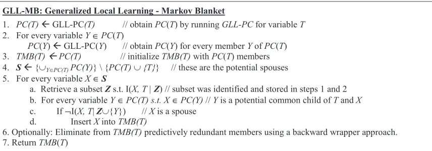
The Generalized Local Learning (GLL) framework consists of two main types of algorithms: GLL-PC (GLL Parent and Children) for Problem 1 and GLL-MB for Problem 2.
4.1 Discovery of the PC(T)Set
Identification of the PC(T)set is based on the following theorem in Spirtes et al. (2000):
Theorem 1 In a faithful BNhV,G,Pithere is an edge between the pair of nodes X∈V and Y ∈V
iff¬I(X,Y|Z), for allZ⊆V \ {X,Y}.
Any variable X that does have an edge with T belongs to the PC(T). Thus, the theorem gives
rise to an immediate algorithm for identifying PC(T): for any variable X∈V \ {T}, and allZ⊆
V \ {X,T}, test whether I(X,T|Z). If such a Z exists for which I(X,T|Z), then X ∈/ PC(T),
otherwise X ∈PC(T). This algorithm is equivalent to a “localized version” of SGS (Spirtes et al.,
2000). The problem of course is that the algorithm is very inefficient because it tests all subsets of the variables and thus does not scale beyond problems of trivial size. The order of complexity is O(|V|2|V|−2
). The general framework presented below attempts to characterize not only the above
There are several observations that lead to more efficient but still sound algorithms. First notice
that, once a subsetZ⊆V \ {X,T}has been found s.t. I(X,T|Z)there is no need to perform any
other test of the form I(X,T|Z′): we know that X∈/ PC(T). Thus, the sooner we identify good
candidate subsetsZthat can render the variables conditionally independent from T , the fewer tests
will be necessary.
Second, to determine whether X ∈PC(T)there is no need to test whether ¬I(X,T|Z)for all
subsetsZ⊆V \ {X,T}but only for all subsetsZ′⊆ParentsG(T)\ {X}and allZ′⊆ParentsG(X)\
{T}where G is any network faithful to the distribution. To see this, let us first assume that there is
no edge between X and T . Notice that either X is a non-descendant of T or T is a non-descendant of X since the network is acyclic and they cannot be both descendants of each other. If X is a
non-descendant of T in G, then by the Markov Condition we know that there is a subset Z of
ParentsG(T) =ParentsG(T)\ {X} (the equality because we assume no edge between T and X )
such that I(X,T|Z). Similarly, if T is a non-descendant of X in G then there isZ⊆ParentsG(X)\
{T} such that I(X,T|Z). Conversely, if there is an edge X →T or T →X , then the dependence
¬I(X,T|Z)holds for allZ⊆V \{X,T}(by the theorem), thus also holds for allZ⊆ParentsG(T)\
{X}orZ⊆ParentsG(X)\ {T}. We just proved that:
Proposition 1 In a faithful BN hV,G,Pithere is an edge between the pair of nodes X ∈V and
T ∈V iff¬I(X,T|Z), for allZ⊆ParentsG(X)\ {T}andZ⊆ParentsG(T)\ {X}.
Since the networks in most practical problems are relatively sparse, if we knew the sets ParentsG(T)and ParentsG(X)then the number of subsets that would need to be checked for con-ditional independence for each X ∈PC(T)is significantly smaller: |2|V\{T,X}|| ≫ |2|ParentsG(X)||+ |2|ParentsG(T)||. Of course, we do not know the sets ParentsG(T) and ParentsG(X) but one could work with any superset of them as shown by the following proposition:
Proposition 2 In a faithful BN hV,G,Pi there is an edge between the pair of nodes X ∈Vand
T ∈V iff¬I(X,T|Z), for allZ⊆SandZ⊆S′, where ParentsG(X)\ {T} ⊆S⊆V \ {X,T}and
ParentsG(X)\ {T} ⊆S′⊆V \ {X,T}.
Proof If there is an edge between the pair of nodes X and T then ¬I(X,T|Z), for all subsets Z⊆V \ {X,T}(by Theorem 1) and so¬I(X,T|Z)for allZ⊆S andZ⊆S′ too. Conversely, if
there is no edge between the pair of nodes X and T , then I(X,T|Z), for someZ⊆ParentsG(X) =
ParentsG(X)\ {T} ⊆SorZ⊆ParentsG(T) =ParentsG(T)\ {X} ⊆S′(by Proposition 1).
Now, the sets ParentsG(X) and ParentsG(T) depend on the specific network G that we are
trying to learn. As we mentioned however, there may be several such statistically equivalent net-works among which we cannot differentiate from the data, forming an equivalence class. Thus, it is
preferable to work with supersets of ParentsG(T)and ParentsG(X)that do not depend on a specific
network member of the class: these supersets are the sets PC(T)and PC(X).
Let us suppose that we have available a superset of PC(T) called TPC(T) (tentative PC). For
any node X∈TPC(T)if I(X,T|Z)for someZ⊆TPC(T)\ {X,T}, then by Proposition 2, we know
that X has no edge with T , that is, X∈/PC(T). So, X should also be removed from TPC(T)to obtain
a better approximation of PC(T). If however,¬I(X,T|Z)for allZ⊆TPC(T)\ {X,T}, then it is
still possible that X∈/PC(T)because there may be a setZ⊆PC(X)whereZ*PC(T)for which
T
A
X
B
PC(T). Notice that, there is no subset of
Figure 3: PC(T) ={A},PC(X) ={A,B},X ∈/ PC(T). Notice that, there is no subset of PC(T)
that makes T conditionally independent of X :¬I(X,T|Ø),¬I(X,T|A). However, there is a subset
of PC(X) for which X and T become conditionally independent: I(X,T|{A,B}). The Extended
PC(T)(see Definition 16 in this section) is EPC(T) ={A,X}.
Is there actually a case, where X cannot be made independent of T by conditioning on some
subset of PC(T)? We know that all non-descendants of T can be made independent of T conditioned
on a subset of its parents, thus, if there is such an X it has to be a descendant of T . Figure 3 shows such a case. These situations are rare in practice as indicated by our empirical results in Sections 5
and 6, which implies that by conditioning on all subsets of TPC(T) one will approximate PC(T)
quite closely.
Definition 16 We call the Extended PC(T), denoted as EPC(T), the set PC(T) union the set of variables X for which¬I(X,T|Z), for allZ⊆PC(T)\ {X}.
The previous results allow us to start building algorithms that operate locally around T in order to
find PC(T)efficiently and soundly. Consider first the sketch of the algorithm below:
Algorithm 1
1: Find a superset TPC(T)of PC(T) 2: for each variable X∈TPC(T)do
3: if∃Z⊆TPC(T)\ {X}, s.t. I(X,T|Z)then
4: remove X from TPC(T) 5: end if
6: end for
7: Return TPC(T)
This algorithm will output TPC(T)⊆EPC(T). To ensure we end up with the exact PC(T)we can
use the following pruning algorithm:
Algorithm 2
1: for all X∈TPC(T)do{returned from Algorithm 1}
2: if T ∈/TPC(X)then
3: remove X from TPC(T){TPC(X)is obtained by running Algorithm 1} 4: end if
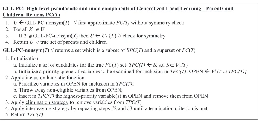
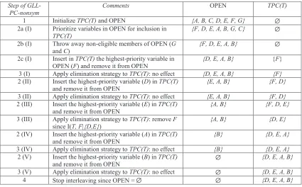
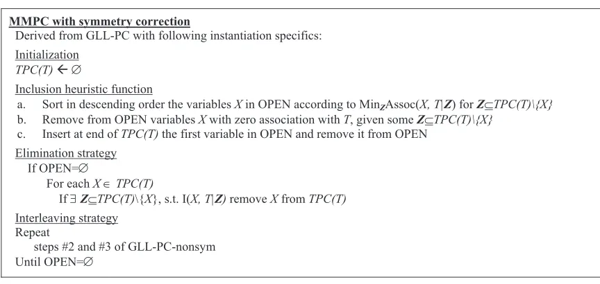
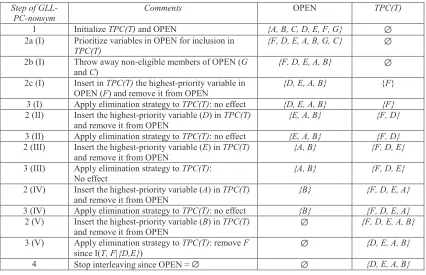
GLL-PC: High-level pseudocode and main components of Generalized Local Learning - Parents and Children. Returns PC(T)
1. Uß GLL-PC-nonsym(T) // first approximate PC(T) without symmetry check 2. For all X U
3. If T GLL-PC-nonsym(X) then U ßU\ {X} // check for symmetry 4. Return U // true set of parents and children
GLL-PC-nonsym(T) // returns a set which is a subset of EPC(T) and a superset of PC(T) 1. Initialization
a. Initialize a set of candidates for the true PC(T) set: TPC(T) ß S, s.t. S V\{T}
b. Initialize a priority queue of variables to be examined for inclusion in TPC(T): OPEN ßV\{T TPC(T)} 2. Apply inclusion heuristic function
a. Prioritize variables in OPEN for inclusion in TPC(T); b. Throw away non-eligible variables from OPEN;
c. Insert in TPC(T) the highest-priority variable(s) in OPEN and remove them from OPEN 3. Apply elimination strategy to remove variables from TPC(T)
4. Apply interleaving strategy by repeating steps #2 and #3 until a termination criterion is met 5. Return TPC(T)
Figure 4: High-level outline and main components (underlined) of GLL-PC algorithm.
In essence, the second algorithm checks for every X ∈TPC(T)whether the symmetrical relation
holds: T ∈TPC(X). If the symmetry is broken, we know that X∈/PC(T)since the
parents-and-children relation is symmetrical.
What is the complexity of the above algorithms? In Algorithm 1 if step 1 is performed by an
Oracle with constant cost, and with TPC(T)equal to PC(T), then the first algorithm requires an
order of O(|V|2|PC(T)|)tests. The second algorithm will require an order of O(|V|2|PC(X)|)tests for
each X in TPC(T). Two observations to notice are: (i) the complexity order of the first algorithm
depends linearly on the size of the problem|V|, exponentially on|PC(T)|, which is a structural
property of the problem, and how close TPC(T)is to PC(T)and (ii) the second algorithm requires
multiple times the time of the first algorithm for minimal returns in quality of learning, that is, just to
take care of the scenario in Figure 3 and remove the variables EPC(T)\PC(T)(i.e., X in Figure 3).
Since an Oracle is not available the complexity of both algorithms strongly depends on how
close approximation of the PC(T)is and how efficiently this approximation is found. The simplest
strategy for example is to set TPC(T) =V, essentially getting the local version of the algorithm SGS
described above. In general any heuristic method that returns a superset of PC(T) is admissible,
that is, it could lead to sound algorithms.
Also notice that in the first algorithm the identification of the members of the TPC(T)(step 1)
and the removal of variables from it (step 3) can be interleaved. TPC(T)can grow gradually by one,
many variables, or all members of it at a time before it satisfies the requirement that is a superset of
PC(T). The requirement for the algorithm to be sound is that, in the end, all tests I(X,T|Z)for all
subsetsZof PC(T)\ {X}have been performed.
Given the above, the components of Generalized Local Learning GLL-PC, that is, an algorithm
for PC(T)identification based on the above principles are the following: an inclusion heuristic