Image Denoising with Kernels Based on Natural Image Relations
Valero Laparra [email protected]
Image Processing Lab, Universitat de Val`encia 46100 Burjassot, Val`encia, Spain.
Juan Guti´errez [email protected]
Dept. Inform`atica, Universitat de Val`encia 46100 Burjassot, Val`encia, Spain.
Gustavo Camps-Valls [email protected]
Jes ´us Malo [email protected]
Image Processing Lab, Universitat de Val`encia 46100 Burjassot, Val`encia, Spain.
Editor: Donald Geman
Abstract
A successful class of image denoising methods is based on Bayesian approaches working in wavelet representations. The performance of these methods improves when relations among the local fre-quency coefficients are explicitly included. However, in these techniques, analytical estimates can be obtained only for particular combinations of analytical models of signal and noise, thus preclud-ing its straightforward extension to deal with other arbitrary noise sources.
In this paper, we propose an alternative non-explicit way to take into account the relations among natural image wavelet coefficients for denoising: we use support vector regression (SVR) in the wavelet domain to enforce these relations in the estimated signal. Since relations among the coefficients are specific to the signal, the regularization property of SVR is exploited to remove the noise, which does not share this feature. The specific signal relations are encoded in an anisotropic kernel obtained from mutual information measures computed on a representative image database. In the proposed scheme, training considers minimizing the Kullback-Leibler divergence (KLD) between the estimated and actual probability functions (or histograms) of signal and noise in order to enforce similarity up to the higher (computationally estimable) order. Due to its non-parametric nature, the method can eventually cope with different noise sources without the need of an explicit re-formulation, as it is strictly necessary under parametric Bayesian formalisms.
Results under several noise levels and noise sources show that: (1) the proposed method out-performs conventional wavelet methods that assume coefficient independence, (2) it is similar to state-of-the-art methods that do explicitly include these relations when the noise source is Gaus-sian, and (3) it gives better numerical and visual performance when more complex, realistic noise sources are considered. Therefore, the proposed machine learning approach can be seen as a more flexible (model-free) alternative to the explicit description of wavelet coefficient relations for image denoising.
1. Introduction
Denoising requires representing the distorted signal in a domain where signal and noise display dif-ferent enough behavior. In such a representation, noise is removed by imposing the known proper-ties of the signal to the distorted samples. In image denoising, classical regularization techniques are used to impose smoothness in the spatial domain since noise is typically white (Banham and Katsaggelos, 1997). Smoothness in the spatial domain means predictability of the signal from the neighborhood, and thus classical approaches exploit the low-pass behavior of the power spectrum to rely on band-limitation or autoregressive models of the signal (Andrews and Hunt, 1977; Banham and Katsaggelos, 1997; Bertero et al., 1988). Several image denoising methods working in the spatial domain have been presented in the literature, either based on splines (Takeda et al., 2007), patch-based approximations (Kervrann and Boulanger, 2007), local auto-regressive models (Guti´errez et al., 2006), or support vector regression (Kai Tick Chow and Lee, 2001; van Ginneken and Mendrik, 2006) to perform smooth (regularized) approximations of the noisy signal. Recently, successful methods use adaptive local basis representations (Dabov et al., 2007). Ap-proaches to the problem using local basis is qualitatively related to wavelet descriptions. In fact, wavelet representations have been recognized as quite appropriate domains for image denoising.1
Wavelet representations are convenient in image denoising because natural image samples have a very specific statistical behavior in this domain. On the one hand, smoothness is represented by a strong energy compaction in coarse scales. On the other hand, the combination of smooth re-gions with local, high contrast features, such as edges, gives rise to sparse activation of wavelet sensors. This leads to very particular, heavy-tailed, marginal probability density functions (PDFs) of the wavelet coefficients (Burt and Adelson, 1983; Field, 1987; Simoncelli, 1997; Hyv¨arinen, 1999). These basic features were incorporated in the classical wavelet-based image denoising tech-niques (Donoho and Johnstone, 1995; Simoncelli, 1999; Figueiredo and Nowak, 2001). Classical techniques such as hard and soft thresholding (Donoho and Johnstone, 1995) have been derived by using Bayesian approaches in non-redundant wavelets, looking for either Maximum a Posteriori (MAP) or Bayesian Least Squares (BLS) estimators, in combination with simple marginal mod-els and assuming statistical independence among coefficients (Simoncelli, 1999; Figueiredo and Nowak, 2001).
It is well-known, however, that marginal models in the wavelet domain are not enough for a proper signal characterization: relevant relations among coefficients still remain after wavelet transforms (Simoncelli, 1999). For instance, edges lead to strong coupling between the energy of neighboring wavelet coefficients of natural images. These relations among wavelet coefficients have proven to be a key issue in applications such as image coding (Malo et al., 2006; Camps-Valls et al., 2008), texture analysis and synthesis (Portilla and Simoncelli, 2000) or image quality metrics (Laparra et al., 2010). The use of these relations is in the roots of the most recent and successful image denoising approaches as well (Portilla et al., 2003; Siwei and Simoncelli, 2007; Goossens et al., 2009). In this case, more complex image models explicitly including the relations among coefficients have to be plugged and fitted into the Bayesian framework to obtain the image estimates.
Unfortunately, all these model-based Bayesian techniques have three common problems:
1. They critically depend on the accuracy of the image model, whose definition is not trivial;
2. MAP or LS estimations can only be derived analytically for particular, typically Gaussian, noise sources. For different noise sources, the whole technique has to be reformulated which may not be analytically tractable;
3. The estimation of the parameters of the image model from the noisy observation is difficult in general.
Conversely, non-parametric approaches can include the above qualitative properties in an indirect way without the restriction of being analytically attached to particular image or noise models. These approaches are based on learning the underlying model directly from the image samples.
In this work we apply support vector regression (SVR) in a redundant (overcomplete) wavelet domain to the noisy image. The proposed method has the following advantages in front of the Bayesian framework:
1. It does not use a particular parametric image model to be fitted, for example, no analytical PDF is required.
2. Its solution may be found for arbitrary noise sources even without knowing the functional form of the noise PDF since it can work with just noise histograms. Therefore, the procedure does not need to be reformulated for different noise sources.
3. It is capable to take into account the relations among wavelet coefficients of natural images through the use of a suitable kernel. In this way, the method preserves the relevant relations among the coefficients of the true signal and better removes the degradation.
The proposed method does not assume independence among the signal coefficients in the wavelet domain, as opposed to Simoncelli (1999) and Figueiredo and Nowak (2001), nor an explicit model of signal relations, as done in Portilla et al. (2003). Therefore, the proposed machine learning approach can be seen as a more flexible (model-free) alternative to the explicit description of wavelet coefficient relations for image denoising. Even though the selection of a particular SVR may be seen as a signal parametrization, the model is still non-parametric in the sense that no functional form of the signal (or noise) characteristics (e.g., the PDF) is assumed.
• Natural images features in redundant wavelet domains. Interesting insight about the
prob-lem can be obtained by analyzing the mutual information between the coefficients of wavelet representations (Buccigrossi and Simoncelli, 1999; Liu and Moulin, 2001). However, in re-dundant domains, it is strictly necessary to discern what are the relations specific to the signal and those due to the transform.
• General constraints of the SVR parameters in image denoising. Generic
recommenda-tions about the SVR parameters have been adapted to propose specific subband-dependent profiles for the insensitivity and the penalization parameters, and to propose a mutual infor-mation based kernel.
• Effect of the SVR parameters. We show the qualitative effect of varying the values of the
parameters under the constrained parameter space.
• Procedure to optimize the SVR parameters. We propose an automatic procedure to select
the SVR parameters based on the Kullback-Leibler divergence, under certain assumptions on signal and noise.
Even though this methodological framework is proposed in the context of achromatic image denois-ing, it can be readily extended to other denoising problems in which wavelet coefficients exhibit particular relations, such as in color or multispectral images, speech signals, etc.
The remainder of the paper is outlined as follows. In Section 2, we point out relevant signal features in redundant wavelet domains through mutual information measurements. These key prop-erties will be used by the proposed algorithm presented in Section 3. In Section 4, the effect of SVR parameters and the validity of the proposed criterion for its selection is addressed experimentally. Section 5 shows the performance of the proposed method compared to standard denoising methods in the wavelet domain. Several experiments dealing with different amount and nature of noise il-lustrate the capabilities of our proposal. Finally, Section 6 draws some conclusions and outlines the further work.
2. Features of Natural Images in the Steerable Wavelet Domain
The starting hypothesis for image denoising is that signal and noise display different characteristics and thus it is possible to separate them in a certain domain. Natural images show non-trivial rela-tionships among wavelet transform coefficients. In the following, we review the reported statistical properties of natural images in orthogonal wavelet domains, and then analyze them in the redundant steerable wavelet domain selected in our implementation. Specifically we will use mutual infor-mation (MI) to assess the statistical relations among wavelet coefficients of natural images as in Buccigrossi and Simoncelli (1999) and Liu and Moulin (2001).
2.1 Intraband Versus Interband Signal Relations in Orthogonal Wavelets
location but in different orientation subbands), or aunts (cousins of the parent). After an exhaus-tive mutual information analysis, the parent provided less information content than the neighbors. These evidences suggest that the dependencies among spatial neighboring coefficients (intraband) in orthogonal wavelet descriptions are stronger than the interband dependencies.
2.2 Natural Images Relations in Steerable Wavelets
Redundant (non-orthogonal) wavelet representations may be more suited to image denoising appli-cations since redundant representation of the image features may make the signal inherent relations clearer. Specifically, some redundant representations are designed to be translation or rotation in-variant (Freeman and Adelson, 1991; Coifman and Donoho, 1995; Kingsbury, 2006). This behavior is convenient to ensure that a particular feature in different spatial regions (or with different orienta-tions) gives rise to the same neighboring relations. Some translation invariant wavelets (Simoncelli and Freeman, 1995) have also a smoother rotation behavior than non-redundant transforms. This justifies applying the same processing all over a particular subband and dealing with the different orientations in similar ways. Besides, this prevents aliasing artifacts appearing in critically-sampled wavelets. In this work we choose a redundant steerable pyramid representation (Simoncelli and Freeman, 1995) to take advantage of these properties.
Despite the reported results on the relations of signal coefficients in orthogonal transforms, a number of questions have to be answered in the case of redundant representations, and in particular, in the steerable wavelet domain:
1. How relevant are the relations among coefficients of natural images in this domain?
2. How relatively important are interorientation, interscale and intraband signal relations?
3. How is the spatial arrangement of these signal relations?
The first question is particularly important since, even though the steerable transform may intensify the relations among signal coefficients, its redundant nature may also introduce relations which could be due to the transform but not to the signal. The second question allows us to focus on the most significant relations. Answering the third question is crucial to design suitable kernels for image denoising.
In the following, we get some insight on these concerns by performing two experiments on a representative database of 920 achromatic images of size 256×256 extracted from the McGill Calibrated Colour Image Database.2
2.2.1 SIGNALRELATIONS ARESPECIFIC TO THESIGNAL
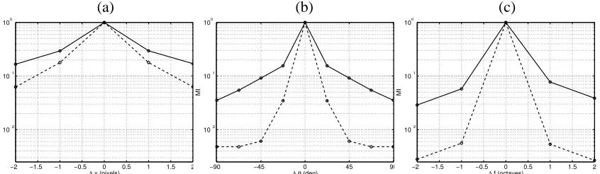
In our first test, following Liu and Moulin (2001), we computed the mutual information among steerable wavelet coefficients of the data set for different spatial, orientation, and scale distances. We used a steerable pyramid with 8 orientations and 4 scales. The mutual information was estimated from the uniformly binned empirical data (256 bins) by computing the histogram of all available sample pairs (721280 samples) for the three considered neighborhoods. In addition, as stated above, in redundant domains it is necessary to know whether these relations come from the images or they are due to the transform. Note that, considering i.i.d. signals, any relation among the coefficients
(a) (b) (c)
Figure 1: Comparison between redundancy of natural image coefficients in the steerable wavelet representation (solid), and the redundancy due to this representation (dashed). Redun-dancy is measured in terms of relative mutual information in logarithmic scale among (a) spatial (b) orientation and (c) scale neighbors.
after a linear transform will be due to the transform no matter their PDF in the original domain. Therefore, in order to assess the amount of relations due to the transform, we compared the MI among natural images coefficients, and the MI among the coefficients of an i.i.d. signal (Fig. 1). The relations displayed by i.i.d. signals in the transformed domain may be seen as a lower bound for the mutual information of signal coefficients. From Fig. 1, it can be noticed that, in every case, relations found in natural images are bigger than those introduced by the transform.
2.2.2 INTRABANDSIGNALRELATIONSDOMINATEOVERINTERSCALE ORORIENTATION
Besides, the results show that intraband relations in the signal are also more important than interor-ientation or interscale relations. Note that mutual information measures are defined to depend on logarithms of probability so that comparisons have to be done by subtraction, not by division. Be-yond consistency with previously reported results for orthogonal wavelet transforms (Buccigrossi and Simoncelli, 1999; Liu and Moulin, 2001), it has been observed that the relations are specific to the signal and not just induced by the transform.
2.2.3 INTRABANDRELATIONS ARESTRONGLYORIENTED
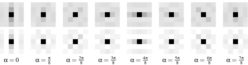
α=0 α=π8 α=2π8 α=3π8 α= 4π8 α=5π8 α=6π8 α=7π8
Figure 2: Mutual information among the central coefficient and its spatial neighbors in the same subband (intraband) in the steerable wavelet domain. Darker gray values indicate higher mutual information. Top row shows the results for the different orientations of the finest scale of the natural image database, and bottom row shows the equivalent results for Gaussian noise.
Summarizing, natural images have singular features in the steerable wavelet domain (Figs. 1 and 2): given a distorted image, enforcing these singular oriented relations among coefficients in every subband (with the appropriate kernels) will eventually preserve the natural signal relations and remove the noise. Of course, the bigger the difference between the shape of the intraband relations in signal and noise the better the results are expected to be.
3. Restoring Wavelet Relations with SVR
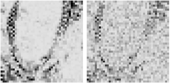
The effect of noise in the wavelet domain is introducing artificial deviations from the original signal and hiding the natural relations among the coefficients (see an illustrative example in Fig. 3). In the more general case, the degraded observation, id, can be written as the result of the addition of a certain realization of noise, n, to the original signal, i:
id=i+n. (1)
Note that this (convenient) way to state the problem does not necessarily mean that the physical degradation has to be additive. In fact, the nature of the degradation should ideally be expressed through a probabilistic noise model that may depend on the original signal, p(n|i). The other de-sirable piece of information is a probabilistic model of the signal, p(i). However, in most practical situations, the complete probabilistic description of the problem, that is, having p(i)and p(n|i), is not available in analytical form.
In order to avoid this lack of information, we propose to use the regularization ability of SVRs. In this section, first we review the capabilities of the SVR for signal approximation. Afterwards, general constraints to the SVR parameter space are given for the particular problem of natural image denoising. Finally, we present an automatic procedure to choose the appropriate SVR parameters (from the above restricted space) to be used for any combination of image and noise.
3.1 Capabilities of SVR for Signal Estimation
Figure 3: Effect of noise on the wavelet coefficients. Patch of a subband of a wavelet representation of the original image Barbara (left) and its noisy version (right). Darker values indicate higher amplitudes.
estimated from the distorted observation, y. Due to the observed strong intraband relations, we will use the SVR in the wavelet domain in patches inside each subband. Subbands are decomposed into non-overlapping 16×16 patches, leading to sets of N=256 samples. Now, given input-output pairs
{pi,yi}Ni=1, where piare the wavelet indices and yiare the corresponding noisy wavelet coefficients
in a patch, we train the adaptive SVR (Camps-Valls et al., 2001; Navia et al., 2001; G´omez et al., 2005) to approximate the signal.
Let φbe a non-linear mapping to a higher dimensional feature space, then the adaptive SVR computes the weights w to obtain the estimation, ˆxi=φ⊤(pi)w, by minimizing the following
regu-larized functional:
kwk2+
∑
i Ciξi,
subject to|yi−φ⊤(pi)w| ≤εi+ξi,∀i=1, . . . ,N, whereξiare the magnitude of the deviations of the
estimated signal from the observed noisy data outside the (sample-dependent) insensitivity zonesεi.
Sample-dependent penalization parameters, Ci, tune the trade-off between fitting the model to the
observed noisy data (minimizing the deviations) and keeping model weightskwksmall (enforcing flatness in the feature space).
This adaptive SVR differs from the standard formulation (Smola and Sch¨olkopf, 2004), in two aspects: (1) the loss function given by (εi,Ci) is sample-dependent, which is convenient in wavelet
domains where signal and noise variances strongly depend on the subband, and (2) the usual bias term in SVM formulations has been intentionally dropped to account for the fact that the expected value of wavelet coefficients is zero. The appropriate design of Ci andεi profiles is analyzed in
Section 3.2.
Explicitly working with the non-linearityφis no longer necessary since the whole formulation can be expressed in the form of dot products of the mapping functions called kernels, K(pi,pj)= φ(pi)⊤φ(pj). In this case, the estimation is given by ˆx = K·α, whereα is the dual representation
case in wavelet domains, we focus on the basic structure of the generalized Radial Basis Functions (RBF) kernel since the relationship among the wavelet coefficients corresponding to spatial neigh-bors within a subband is local. However, as it will be analyzed in Section 3.2, the kernel will be adapted to incorporate the anisotropic signal relations studied in Section 2.2, see Fig. 2.
3.2 General Constraints on SVR Parameter Space in Image Denoising
As stated above, SVR signal approximation will depend on the penalization parameters, Ci, the
insensitivities, εi, and the kernel K. In the following, we restrict the range of possible values of
these parameters,θ= (Ci,εi,K), in the particular case of image denoising in wavelet domains:
Penalization factor. In general, the penalization factor of SVRs should be related to the standard
deviation of the signal (Cherkassky, 2004). In the denoising problem considered here, the signal variance substantially differs in each wavelet scale. According to this, it is strictly nec-essary to set a different penalization factor per scale, Ci=C ki, where kiis a scale-dependent
profile. This profile ki was obtained by averaging the standard deviation of wavelet
coeffi-cients over 100 images from the database used in Section 2. This profile was multiplied by a factor, C, varied in the range [10, 104], which did not show a strong impact on the results provided a sufficiently large value. This is consistent with the suggestions reported in Chal-imourda et al. (2004) in a more general context. Note that, for instance, in the examples of the next section (Fig. 3), indistinguishable results are obtained for a large enough C. In our experiments, we found that a reasonable prescription for the global factor on the penalization profile is C≈103.
Adaptive insensitivity zone. In general, the insensitivity has to be related to the standard deviation
of the noise (Kwok and Tsang, 2003). In transformed domains, the effect of the transform has to be taken into account in order to estimate the corresponding standard deviation. In redundant wavelet representations, this standard deviation is coefficient dependent. Thus it is strictly necessary to introduce a subband-dependentεi profile (Camps-Valls et al., 2001;
G´omez et al., 2005). The transformed standard deviations can be estimated either (1) empir-ically from noise samples, or (2) computed from the noise covariance matrix if it is known. In the empirical case, noise samples can be experimentally obtained by applying the noise source to a large enough set of images, and writing the noise as in Eq. 1. In our experiments, we used the natural image database used in Section 2, and we obtained fairly stable results for the profile by considering 100 images. In the case that the noise covariance is known, the cor-responding matrix in the selected wavelet domain can be obtained from the noise covariance matrix in the spatial domain,Σn, and the transform T (Stark and Woods, 1994). Therefore,
the insensitivity profile can be computed as:
εi=τdiag(T·Σn·T⊤)1i/2. (2)
In the case of white noise,Σn=σ2n·I, and thus Eq. (2) reduces to:
εi=τ σndiag(T·T⊤)1i/2, (3)
α=0 α=π8 α=2π8 α=3π8 α= 4π8 α=5π8 α=6π8 α=7π8
Figure 4: Anisotropic kernel functions used in the support vector regression method for the eight considered orientation subbands.
[0.5, 3] according to the known relationship between the ε-insensitivity zone and the noise standard deviation (Kwok and Tsang, 2003). Note that (2) may cope with colored noise. Con-sidering the off-diagonal elements of the covariance matrix (neglected in (2) and (3)) would give rise to couplingε-insensitivities among samples. This issue has been already considered and solved in the context of image coding by using an additional non-linear transform and a constantεin the transformed domain (Camps-Valls et al., 2008). However, in this paper, we restrict ourselves to the approximated diagonal case.
Including signal relations in the kernel. In the kernel methods literature, the use of prior
knowl-edge about the problem can be encoded through bagged, cluster, or probabilistic kernels (Je-bara et al., 2004; Weston et al., 2004). In our case, we propose to take into account image coefficient relations by analyzing a large (representative) database and taking the (oriented) mutual information among samples as core distance measure. However, using these empiri-cal measures to set the kernels is not straightforward since the kernels have to fulfill Mercer’s Theorem (Mercer, 1905). According to this, we propose to use generalized Gaussian ker-nels. In particular, we fitted anisotropic Laplacian kernels to the MI measures to consider the intraband oriented relations within each subband:
Kα(pi,pj) = exp −((pi−pj)⊤G(α)⊤Σ−1G(α)(pi−pj))1/2
,
whereΣ=
σ
1 0
0 σ2
,σ1andσ2are the widths of the kernels, pi∈R2denotes the spatial
position of coefficient yi within a subband, and G(α)is the 2D rotation matrix with rotation
angle,α, corresponding to the orientation of each subband (see Fig. 4). Note that these set of oriented kernels describe the signal relationships that emerge from experiments in Section 2 (cf. Fig. 2[top]).
We obtained proper values for the widthsσ1andσ2by fitting the above kernel to the MI mea-sures among coefficients described in Section 2 (σ1=2σ2, andσ1=4.8 in spatial coefficient units). The kernel was further normalized in the standard way. Since this width comes from direct measures from images, it describes a fundamental property of natural images so it can be kept fairly constant.
3.3 Procedure for Automatic SVR Selection
In the more general case, applying SVRs with a given set of parameters,θ, to a noisy image leads to a certain image estimate, ˆiθ=T−1·ˆxθ. From this image estimate, and the convenient additive notation for the noise (Eq. (1)), a noise estimate can be obtained: ˆnθ=id−ˆiθ. In this section we propose a procedure to select the SVR parameters,θ, that better approximates the noise free image, using the available information.
In the more general situation the only available information is the noisy image. However, as stated above, denoising methods usually assume that additional probabilistic information on the signal and noise is available: p(i)and p(n|i). Note that this knowledge is equivalent to the knowl-edge of the joint signal and noise distribution since p(i,n) =p(n|i)p(i).
Let us momentarily assume that this information is available to propose the general procedure to set the SVR parameters. Afterwards, we will relax the requirements by considering an approxi-mation that can be easily applied in practical situations.
In order to enforce solutions that closely follow the (assumed to be known) statistics of signal and noise, we propose to select the SVR that minimizes the k-th order Kullback-Leibler divergence (KLD) (Cover and Tomas, 1991) between the joint PDF of signal and noise, and the joint PDF of the estimated signal and the estimated noise:
θ∗=arg min θ
DKL
p(ˆiθ,ˆnθ) k p(i,n)
. (4)
The underlying idea is that the SVR that minimizes the divergence between the above PDFs is the one that better captures the features of the true signal and better removes the degradation.
Although in ideal situations the application of this procedure would obtain the best results in statistical terms, in practical situations the full probabilistic description of the problem is not avail-able. A number of approximations are done in practical situations. For instance, thermal noise in CCD cameras is not independent from the input signal since diffusion increase with the irradi-ance. However, thermal noise is usually assumed to be independent of the input signal. Additional assumptions as additivity or certain analytical marginal PDF of the noise are also widely used.
In our case, we assume independence between signal and noise:
p(i,n) =p(i)p(n).
However, no analytical model for these PDFs is assumed. Under this independence assumption, it is easy to see that Eq. 4 reduces to:
θ∗=arg min θ
DKL
p(ˆiθ) k p(i)
+DKL
p(ˆnθ)k p(n)
. (5)
This means that the selected SVR parameters are those that give rise to both signal and noise es-timates probabilistically similar to the true signal and noise respectively. Note that this similarity does not require analytical models of the PDFs since it can be computed from histograms (or signal and noise samples).
histogram estimations of p(i)and p(n)are far more reliable than histogram estimations of p(i,n), which implies the duplication of the dimensionality (in an already high dimensional situation).
In the examples throughout the paper we restricted ourselves to second order KLD measures due to the lack of samples, yet capturing the second order structure of signal and noise. The optimization in Eq. (5) was carried out by exhaustive search.
3.4 Summary of the Proposed Denoising Method
The proposed denoising method can be summarized as follows. First the noisy image is transformed by a steerable wavelet filter bank. Then, a set of SVRs is applied to the patches of the subbands of the transform. These SVRs use the profiles for the penalization factor and the insensitivity computed from signal and noise samples as described in Section 3.2. The SVRs use the kernel based on MI that captures signal relations in the wavelet domain as described in Section 3.2. While the scaling of the penalization profile and the kernels are kept fixed as indicated in Section 3.2, the scaling of the insensitivity profile is automatically selected following the procedure described in section 3.3.
4. Behavior of the Proposed Method
In this section, we show an illustrative example of how the SVR parameters affect the estimated solution. Moreover we validate the proposed automatic procedure for SVR selection considering examples with different noise sources including non-additive and signal dependent cases.
4.1 Impact of SVR Parameters in Image Denoising
As stated above, the regularization behavior of the SVR depends onθ= (Ci,εi,K). Here we show
the qualitative effect of the global penalization scaling C, the global insensitivity scaling τ, and the kernel width σ assuming a generalized RBF kernel. Figure 5 shows the qualitative effect of SVR estimation as a function of these parameters. Compare the results with the original and noisy subbands shown in Fig. 3.
Increasing the kernel width,σ(vertical direction), introduces too strong relations among coeffi-cients in such a way that spurious energy appears in the reconstruction. Increasing the insensitivity,
τ(horizontal direction), a sparser solution is obtained, leading to information loss and thus relevant features of the signal are discarded. On the contrary, a too small insensitivity value gives rise to overfitting, and hence noise is not removed. Small values of the C parameter gives rise to over-regularized estimations. Large enough values of C give rise to similar behavior (see comments in Section 3.2).
Of course, interactions among these parameters occur, and have been studied in other contexts elsewhere (Chalimourda et al., 2004; Cherkassky and Ma, 2003; Cherkassky, 2004). In the image denoising case, the deviation from an appropriate solution in combined directions of the parameters gives rise to different solutions that combine the negative effect of the departure in each direction.
The above example suggests that appropriate SVRs can certainly recover the underlying struc-ture of the original signal from the noisy observation, which is the rationale of the proposed method.
4.2 Validation of the Automatic Procedure for SVR Selection
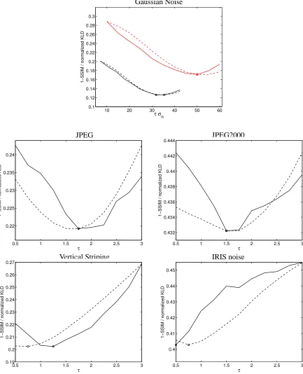
Figure 5: Effect of SVR parameters on the noisy wavelet patch of Fig. 3. The values of the KL-divergence criterion between the estimated and the actual PDFs of noise and signal are given in each case (see text in Section 3.3).
procedure: the minimum divergence solution (central subband patch) gives also a reasonable trade-off between smoothness and detail preservation of the original subband patch.
Secondly, we quantitatively show that the SVR that enforces the similarity between the esti-mated and actual signal and noise joint PDFs (in KLD terms) is not far from the SVR that maxi-mizes the structural similarity between the estimated and the original image. In order to do so, we compare the KLD measures for different SVRs, with the corresponding distortion measured with the Structural SIMilarity (SSIM) index (Wang et al., 2004). The SSIM index is a widely used simi-larity measure, which is better related to human quality assessment than Euclidean measures, such as MSE or PSNR. Note that while KLD values are available in real situations (provided the noise histogram and a generic natural images histogram are known), distortion measures are not available since the original image is unknown. Consequently, the SSIM results next presented are for mere comparison purposes.
In this experiment, the SVM parameter space is reduced to the scaling factor on the insensitivity profile as recommended in Section 3.2. Accordingly, Fig. 6 shows the KLD and distortion (1-SSIM) results as a function ofτ(see Eq. (3)). Curves are shown for different kinds of (Gaussian and non-Gaussian) noise sources corrupting a particular image (details on the noise sources are given in Section 5).
(red curves) the higher the ε zone minima. Besides, the linear relation between ε and the noise standard deviation, reported in Kwok and Tsang (2003), is confirmed here: as expected, the scaling factor keeps fairly constant, τ≈2.5, for bothσ2n=200 and σ2n=400. Obviously, higher noise levels imply more distorted estimations. For other (non-Gaussian) noise sources, similar results are obtained. For the JPEG and JPEG2000 quantization noise sources, the KLD criterion also matches SSIM performance. For the case of more complex noise sources, such as vertical striping (VS) and Infra Red Imaging System (IRIS) noise, the criterion gives close-to-optimal solutions in SSIM terms. Note that, remarkably, the KLD criterion is better suited to the error minimization when the signal and noise independence assumption holds (Gaussian case). Therefore there is room to further improve the SVR selection criterion. The above results suggest that the proposed SVR selection procedure can be considered as a convenient approximation to distortion minimization (which is not possible in real situations).
5. Denoising Experiments and Discussion
In this section, we evaluate the performance of the proposed method in different scenarios for image denoising. Our algorithm is compared to several wavelet-based denoising methods using standard 256×256 images (‘Barbara’, ‘Boats’, ‘Lena’) with different levels and sources of degradation. In the following, we first give details on implementation issues of the considered algorithms. Then, we analyze their performance for several kinds of noise sources:
• Experiment 1. Additive Gaussian noise of different variances (σ2n={200,400}).
• Experiment 2. Coding noise: JPEG and JPEG2000 at different quantization coarseness.
• Experiment 3. Acquisition noise: vertical striping and Infra Red Imaging System (IRIS) noise.
Note that the noise PDF is in general unknown, except for the academic case of Gaussian noise, but the histogram can be computed from samples in all cases.
All results are compared numerically by using the standard (yet not perceptually meaningful) RMSE, and the perceptually meaningful SSIM index (Wang et al., 2004). Moreover, representative exam-ples are shown in every case for visual inspection. For proper visualization, all the results are equalized in the same way by truncating the values outside the[0,255]range.
5.1 Implementation Details
The algorithms that do not use information about the inter-coefficient relations (Donoho and John-stone, 1995; Simoncelli, 1999; Figueiredo and Nowak, 2001) are straightforward to implement and have few parameters to tune. All these methods use orthogonal wavelet representations. In our particular implementation, we used 4-scale QMF wavelets from MatlabPyrTools.3 In every case, we followed authors’ prescriptions to choose these parameters for the best performance:
• Hard Thresholding (HT). The key parameter is the threshold valueλ. We use the noise vari-ance to set the threshold,λ=3σn, as suggested in Donoho and Johnstone (1995).
JPEG JPEG2000
Vertical Striping IRIS noise
• Soft Thresholding (ST). In our implementation, the threshold in each subband is derived from
the standard deviation of the noise,σn, using optimized values to minimize the mean square
error (MSE) in a set of 100 natural images. Threshold values were optimized for theσ2nin the range [0,1600].
• Bayesian Laplacian (BL). In this case, the parameters of the Laplacian distribution (s and p in Simoncelli, 1999) for the marginal PDFs in each subband are estimated by maximum
likelihood (ML), as suggested by the author.
• Bayesian Gaussian (BG). The threshold value was set according to the function of noise
variance provided in Figueiredo and Nowak (2001).
On the other hand, in the case of the Gaussian Scale Mixture (GSM) (Portilla et al., 2003), which does consider inter-coefficient relations, we used the implementation provided by the authors.4 We have used (1) the same representation as in the proposed method (4-scale, 8-orientation steerable pyramid), and (2) we also provided the average noise power spectral density (PSD) to achieve the best possible performance of the GSM method.
Details of the proposed SVR method are included in previous Section 3.2. A Matlab imple-mentation of the algorithm is available online.5 Since the Ci andεiprofiles are computed off-line,
the computational cost of the proposed method is mainly constrained by the SVR training. In our current implementation, we used the IRWLS algorithm in Matlab (P´erez-Cruz et al., 2000) in order to drop the bias term and incorporate the insensitivity and penalization profiles easily. These modi-fications are not trivial in faster implementations (Huang and Kecman, 2004; Kecman et al., 2004). As a result, our Matlab implementation takes about 30 seconds6 for each image/noise estimation for a set of SVR parameters. Three strategies can be carried out for speeding up the optimization: (1) using faster SVR implementations (Platt, 1999; Chang and Lin, 2001; Tsang et al., 2005), (2) alternative procedures to exhaustive search on convex error surfaces (Torczon, 1997; Lewis and Tor-czon, 2002; Vishwanathan et al., 2006), and (3) restricting the dimension of the parameter space (as done in Section 3.2).
5.2 Experiment 1. Additive Gaussian Noise
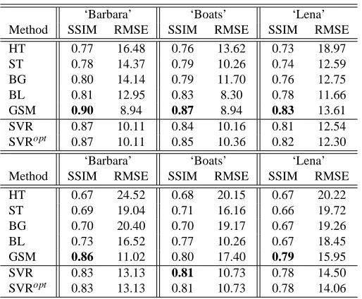
Table 1 shows the distortion results for the three considered images and the two noise variances,
σ2
n=200 andσ2n=400.. The best SSIM values in each case are highlighted. In every case, we
also provide the SVRopt result, which is the best result the proposed method can get in SSIM terms. This is useful to assess the performance of the proposed divergence-based criterion and to give an upper bound of method’s performance. Results show that our algorithm performs better than the methods that neglect signal relations (HT, ST, BG and BL), and obtains similar (yet slightly lower) numerical results than the one which incorporates them (GSM). It is not surprising that the GSM method achieves the best performance in this case, since it is analytically suited to deal with Gaussian noise. The SVR performance is consistent through all images and noise variances, thus suggesting that the guiding criterion is robust. Finally, it must be noted that, in the most difficult case ofσ2n=400, GSM and SVR offer more similar results, and clearly outperform the rest of the methods.
4. Seehttp://decsai.ugr.es/˜javier/denoise/.
‘Barbara’ ‘Boats’ ‘Lena’ Method SSIM RMSE SSIM RMSE SSIM RMSE HT 0.77 16.48 0.76 13.62 0.73 18.97 ST 0.78 14.37 0.79 10.26 0.74 12.59 BG 0.80 14.14 0.79 11.70 0.76 12.75 BL 0.81 12.95 0.83 8.30 0.78 11.66 GSM 0.90 8.94 0.87 8.94 0.83 13.61 SVR 0.87 10.11 0.84 10.16 0.81 12.54 SVRopt 0.87 10.11 0.85 10.36 0.82 12.30
‘Barbara’ ‘Boats’ ‘Lena’ Method SSIM RMSE SSIM RMSE SSIM RMSE HT 0.67 24.52 0.68 20.15 0.67 20.22 ST 0.69 19.04 0.71 16.16 0.66 19.72 BG 0.70 20.40 0.70 19.17 0.67 19.26 BL 0.73 16.52 0.77 10.26 0.67 18.45 GSM 0.86 11.02 0.80 17.40 0.79 15.95 SVR 0.83 13.13 0.81 10.73 0.78 14.50 SVRopt 0.83 13.13 0.81 10.73 0.78 14.06
Table 1: Results for the Gaussian noise: distortions for different images and methods are given at
σ2
n=200 (top) andσ2n=400 (bottom).
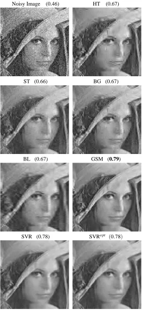
Figure 7 shows representative visual results in the challenging situation of σ2n=400. It can be noticed that thresholding methods (HT, ST) and Bayesian generalizations not including signal relations in the model (BG, BL) show poor performance, producing images either grained or cor-rupted by too salient wavelet functions. Even though SVR yields slightly lower numerical scores than GSM, global visual performance is comparable.
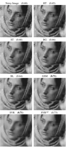
5.3 Experiment 2. Coding Noise: JPEG and JPEG2000
In this section, we focus on restoring grayscale images after JPEG or JPEG2000 compression, which induces non-Gaussian noise: it produces heavy tailed marginal error PDFs in the spatial domain with non-negligible relations among the pixels (see comments in Section 5.5). Quantization noise is an illustrative example of how the proposed method can cope with non-Gaussian, colored and signal-dependent noise. In order to obtain the necessary samples to build the noise histograms, we used 100 images from the database described in Section 2 encoded by JPEG and JPEG2000. In the first case, the Matlab implementation of the JPEG algorithm with quality factors Q=9 (small distortion) and Q=7 (large distortion) was used. In the second case, scalar quantization of the QMF wavelet domain using standard JPEG2000 bit allocation tables (Taubman and Marcellin, 2001) was used. Different values of quantization coarseness, that will be referred to as∆1(small distortion) and∆2 (large distortion) were applied.
ST (0.66) BG (0.67)
BL (0.67) GSM (0.79)
SVR (0.78) SVRopt (0.78)
ST (0.68) BG (0.66)
BL (0.64) GSM (0.71)
SVR (0.71) SVRopt (0.73)
ST (0.55) BG (0.54)
BL (0.54) GSM (0.55)
SVR (0.57) SVRopt (0.57)
JPEG Q=9 Q=7
‘Barbara’ ‘Boats’ ‘Lena’ ‘Barbara’ ‘Boats’ ‘Lena’ Method SSIM RMSE SSIM RMSE SSIM RMSE SSIM RMSE SSIM RMSE SSIM RMSE HT 0.70 20.05 0.75 13.07 0.70 18.40 0.65 22.11 0.71 16.34 0.65 24.99 ST 0.73 17.51 0.78 11.59 0.73 15.13 0.68 19.71 0.75 12.72 0.68 18.77 BG 0.72 18.76 0.77 12.30 0.72 16.27 0.66 21.57 0.74 13.32 0.67 21.05 BL 0.71 20.37 0.77 13.43 0.73 16.52 0.64 21.67 0.74 14.70 0.69 17.65 GSM 0.77 15.50 0.80 11.15 0.75 13.66 0.71 18.56 0.77 12.18 0.71 17.45 SVR 0.78 14.89 0.78 12.13 0.74 13.22 0.71 18.42 0.76 12.84 0.71 15.68 SVRopt 0.78 14.89 0.80 11.35 0.75 13.97 0.73 18.28 0.76 12.89 0.71 15.72
JPEG2000 ∆2 ∆1
‘Barbara’ ‘Boats’ ‘Lena’ ‘Barbara’ ‘Boats’ ‘Lena’ Method SSIM RMSE SSIM RMSE SSIM RMSE SSIM RMSE SSIM RMSE SSIM RMSE HT 0.54 30.81 0.55 26.23 0.51 32.66 0.67 24.82 0.59 25.18 0.56 28.25 ST 0.55 28.83 0.55 25.15 0.51 31.24 0.68 22.52 0.60 23.69 0.56 27.47 BG 0.54 30.37 0.55 26.08 0.51 32.45 0.67 24.16 0.59 24.92 0.56 28.10 BL 0.54 30.30 0.55 25.87 0.51 29.05 0.67 24.35 0.59 24.79 0.56 28.12 GSM 0.55 28.47 0.57 20.92 0.52 25.84 0.68 20.54 0.64 17.94 0.58 23.64 SVR 0.57 25.31 0.57 21.88 0.52 29.32 0.71 17.23 0.64 18.27 0.59 21.55 SVRopt 0.57 25.31 0.57 21.74 0.52 25.35 0.72 17.04 0.64 18.27 0.59 21.55
Table 2: Results for the coding noise: distortions at different quality levels of JPEG (Q={9,7}) and JPEG2000 (coarseness∆1and∆2) are given for different images and methods.
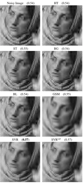
5.4 Experiment 3. Acquisition Noise: Vertical Striping and IRIS Noise
Real imaging systems introduce complex forms of noise depending on the acquisition process, so assuming a particular PDF for all cases is far from being realistic. For instance, variation of the intensity between neighboring elements of the CCD typically leads to vertical striping noise in pushbroom sensors (Mouroulis et al., 2000; Barducci and Pippi, 2001). Other typical acquisition noise source is observed in infrared imaging cameras, which is a complex mixture of different noise sources. In this section, we pay attention to these two particular non-Gaussian realistic acquisition noises through controlled experiments:
1. Vertical striping noise. We simulated this noise by modifying 4% of the image columns selected randomly. The luminance of the selected columns was modified by a random factor following a uniform distribution between 0.8 and 1. Spatial coherence was forced by attaching groups of contiguous 5 to 10 strips.
2. InfraRed Imaging System (IRIS) noise. Inspired in the observed characteristics of a represen-tative number of acquired images by a commercial IR camera, the noise was modeled by a combination of four noise sources: low-variance Gaussian noise (σ2
n≈50), ‘salt-and-pepper’
noise (with a percentage of corrupted pixels about 0.05%), some spatially coherent missing pixels (black patches), and interlaced lines all over the image.
In both cases, we computed the contrast noise PDF, p(n), from 100 noisy images. In the next Section 5.5, the non-Gaussian nature of these acquisition noise PDFs is shown.
Method ‘Barbara’ ‘Boats’ ‘Lena’ SSIM RMSE SSIM RMSE SSIM RMSE HT 0.73 17.43 0.73 15.99 0.69 18.07 ST 0.77 15.71 0.78 14.04 0.75 14.08 BG 0.76 16.01 0.76 14.75 0.73 15.14 BL 0.77 16.56 0.81 14.96 0.77 14.64 GSM 0.79 14.83 0.79 14.36 0.75 14.45 SVR 0.80 15.66 0.80 13.47 0.79 13.18 SVRopt 0.80 15.45 0.82 14.25 0.80 13.31 HT 0.50 30.80 0.58 28.70 0.56 28.81 ST 0.55 27.02 0.64 23.48 0.60 24.40 BG 0.54 28.40 0.62 25.44 0.59 26.20 BL 0.50 28.74 0.60 21.77 0.55 24.08 GSM 0.53 30.51 0.64 25.92 0.61 30.99 SVR 0.59 31.07 0.67 21.44 0.66 31.44 SVRopt 0.60 30.71 0.70 24.56 0.66 32.05
Table 3: Acquisition noise: vertical striping (top) and IRIS noise (bottom). Distortions for different images and methods.
methods numerically. A noticeable gain in SSIM is observed, which is confirmed when looking at the restored images in Figs. 10 and 11. It is worth noting that in the vertical striping noise (Fig. 10), SVR yields a sharper (and more realistic) reconstruction while GSM produces an over-blurred solution. In the case of the IRIS noise, only SVR removes the interlacing noise contribution, producing better visual results. Including the average PSD information in GSM, as we do in the experiments, improves its performance. However, it is not enough to remove the interlacing artifact due to the particular nature of IRIS noise. IRIS noise is difficult because the PSD and variance of each particular realization of the noise may substantially differ from the (estimated) averages. On the contrary, the proposed SVR method uses an adaptive cost function learned from the noisy image. Here, nevertheless, the upper bound of performance is not met, suggesting that there is still room for improving the selection criterion proposed, possibly considering the joint density.
5.5 Analysis of the Residuals
Further qualitative insight in the obtained solutions can be achieved by comparing the estimated and actual PDFs of signal and noise with the different methods and noise sources. Since we are restricting ourselves to second order KLD criterion, this comparison reduces to assess the difference between 2D histograms (in the spatial domain).
ST (0.75) BG (0.73)
BL (0.77) GSM (0.75)
SVR (0.79) SVRopt (0.80)
ST (0.64) BG (0.62)
BL (0.60) GSM (0.64)
SVR (0.67) SVRopt (0.70)
suitable for direct inspection because (1) actual noise histograms are quite different for the different noise sources, and (2) the estimated histograms strongly depend on the denoising method.
Figure 4 represents the distribution of the actual and estimated noise PDFs by all the considered methods in the spatial domain. It can be noticed that, for the Gaussian noise, all methods reproduce quite well the shape and extent of the PDF, as expected for the parametric models, which use a proper Gaussian noise model. Note that the SVR method also succeeds in approximating the energy of the noise even without using the Gaussian assumption explicitly.
For non-Gaussian noise sources, the behavior of the methods markedly differ. For instance, the quantization noise induced by JPEG/JPEG2000 follows a non-Gaussian, oriented joint distribution (the central dark area is actually an oriented ellipsoid), indicating correlation among noise samples. In the case of JPEG, this central ellipsoid is better reproduced by hard thresholding and the proposed SVR method. The other methods slightly underestimate the variance of the noise. For the case of JPEG2000, methods not considering signal relations dramatically underestimate the noise variance. In the case of more complex noise sources, such as vertical striping or IRIS, none of the methods reproduce the low probability structure (light gray regions). However, the central peak is poorly reproduced by marginal methods, either overestimating (HT, ST, BG) or underestimating (BL) the width. On the contrary, GSM and SVR give more reasonable width estimation. To conclude, meth-ods assuming an (inadequate) Gaussian noise model do not match, in general, the noise distribution, so they should be reformulated for each particular noise source, which may be complicated or even impossible. GSM constitutes an exception to this statement, since results suggest that the quality of the signal model compensates the unsuitability of the noise model. On the contrary, this is not necessary for the proposed method, which only needs examples of noisy images to learn from.
6. Conclusions
In this work, we proposed an alternative non-parametric way to take into account the relations among natural image wavelet coefficients for denoising: we used SVR in the wavelet domain to en-force these relations in the estimated signal. The specific signal relations, which proved to be more relevant in intraband coefficients, are encoded in an anisotropic kernel based on mutual information computed from a representative image database. An adaptive SVR with different cost function per subband was developed: the subband-dependentεi and Ci are modeled by analyzing the particular
signal and noise variances in a representative image database. By following general recommenda-tions for the design of the kernel, εi and Ci, and adapting them to the particular image denoising
problem, we restricted the class of appropriate SVRs. A KLD-based criterion was proposed to au-tomatically select the SVR that best recovers the relevant wavelet coefficient relations of the true signal. The criterion was quite consistent but there is still room for improvement, specially in the case of complex noise sources.
S p atia l N o is e H T S T B G B L G S M S V R
additional indication that relation between local frequency coefficients is a salient natural image feature that should not be neglected in denoising applications.
Future work is tied to the incorporation of new information in the kernels: here we focused on the consideration of signal relations in the kernel, but the particular structure of the noise could be eventually incorporated. Note that the denoising procedure is quite general and admits any kind of non-parametric regression machine, such as Gaussian Processes.
Acknowledgments
This work was partially supported by projects CICYT-FEDER TEC2009-13696, AYA2008-05965-C04-03, and CSD2007-00018. Valero Laparra acknowledges the support of the Ph.D grant BES-2007-16125. The authors thank the reviewers for thorough and constructive comments on the sub-mitted manuscript.
References
H.C. Andrews and B.R. Hunt. Digital Image Restoration. Prentice Hall, NY, 1977.
M. Banham and A. Katsaggelos. Digital image restoration. IEEE Signal Processing Magazine, 14: 24–41, 1997.
A. Barducci and I. Pippi. Analysis and rejection of systematic disturbances in hyperspectral re-motely sensed images of the Earth. Applied Optics, 40:1464–1477, 2001.
A. J. Bell and T. J. Sejnowski. The ‘independent components’ of natural scenes are edge filters.
Vision Research, 37(23):3327–3338, 1997.
M. Bertero, T.A. Poggio, and V. Torre. Ill-posed problems in early vision. Proceedings of the IEEE, 76(8):869–889, 1988.
R. W. Buccigrossi and E. P. Simoncelli. Image compression via joint statistical characterization in the wavelet domain. IEEE Transactions on Image Processing, 8(12):1688–1701, 1999.
P. J. Burt and E. H. Adelson The Laplacian Pyramid as a compact image code. IEEE Transactions
on Communications, 31(4):532–540, 1983.
G. Camps-Valls, E. Soria-Olivas, J. P´erez-Ruixo, A. Art´es-Rodr´ıguez, F. P´erez-Cruz, and A. Figueiras-Vidal. A profile-dependent kernel-based regression for cyclosporine concentration prediction. In Neural Information Processing Systems (NIPS) – Workshop on New Directions in
Kernel-Based Learning Methods, Vancouver, Canada, December 2001.
G. Camps-Valls, J. Guti´errez, G. G´omez, and J. Malo. On the suitable domain for SVM training in image coding. Journal of Machine Learning Research, 9:49–66, 2008.
C. Chih Chang and Chih J. Lin. libSVM: A Library for Support Vector Machines,
(http://www.csie.ntu.edu.tw/˜cjlin/libsvm/), 2001.
H. Cheng, J.W. Tian, J. Liu, and Q.Z. Yu. Wavelet domain image denoising via SVR. IEE
Electron-ics Letters, 40, 2004.
V. Cherkassky. Practical selection of SVM parameters and noise estimation for SVM regression.
Neural Networks, 17(1):113–126, 2004.
V. Cherkassky and Y. Ma. Comparison of model selection for regression. Neural Comput., 15(7): 1691–1714, 2003.
R.J. Clarke. Transform Coding of Images. Academic Press, New York, 1985.
R. R. Coifman and D. L. Donoho. Translation-invariant de-noising. In A. Antoniadis and G. Oppen-heim, editors, Wavelets and Statistics. Lecture Notes in Statistics, volume 103, pages 125–150. Springer, Berlin, Department of Statistics, 1995.
T.M. Cover and J.A. Tomas. Elements of Information Theory. John Wiley & Sons, New York, 1991.
K. Dabov, A. Foi, V. Katkovnik, and K. Egiazarian. Image denoising by sparse 3D transform-domain collaborative filtering. IEEE Transactions on Image Processing, 16(8):2080–2095, 2007.
D. L. Donoho and I. M. Johnstone. Adapting to unknown smoothness via wavelet shrinkage. Journal
of the American Statistical Association, 90:1200–1224, 1995.
D. Field. Relations between the Statistics of Natural Images and the Response Properties of Cortical Cells. Journal of the Optical Society of America A, 4(12):2379–2394, 1987.
M. Figueiredo and R. Nowak. Wavelet-based image estimation: an empirical Bayes approach using Jeffrey’s noninformative prior. IEEE Transactions on Image Processing, 10(9):1322–1331, 2001.
W. T. Freeman and E. H. Adelson. The design and use of steerable filters. IEEE Pattern Analysis
and Machine Intelligence, 13(9):891–906, 1991.
G. G´omez, G. Camps-Valls, J. Guti´errez, and J. Malo. Perceptual adaptive insensitivity for support vector machine image coding. IEEE Transactions on Neural Networks, 16(6):1574–1581, 2005.
B. Goossens, and Pizurica, A. and Philips, W. Removal of correlated noise by modeling the signal of interest in the wavelet domain. IEEE Transactions on Image Processing, 18(6):1153–1165, 2009.
J. Guti´errez, F. Ferri, and J. Malo. Regularization operators for natural images based on nonlinear perception models. IEEE Transactions on Image Processing, 15(1):189–200, 2006.
T.-M. Huang and V. Kecman. Bias term b in SVMs again. In 12th European Symposium on Artificial
Neural Network, ESANN 2004, pages 441–448, Bruges, Belgium, April 2004.
A. Hyvarinen, J. Karhunen, and E. Oja. Independent Component Analysis. John Wiley & Sons, New York, 2001.
T. Jebara, R. Kondor, and A. Howard. Probability product kernels. Journal of Machine Learning
Research, 5:819–844, 2004.
D. Kai Tick Chow and T. Lee. Image approximation and smoothing by support vector regression. In International Joint Conference on Neural Networks, IJCNN’01., volume 4, pages 2427–2432, Washington, DC, USA, 2001.
V. Kecman, T. Huang, and M. Vogt. Iterative single data algorithm for training kernel machines from huge data sets: Theory. In Performance, Support Vector Machines: Theory and Applications,
Springer-Verlag, Studies in Fuzziness and Soft Computing, p 255–274, 2004.
C. Kervrann and J. Boulanger. Local adaptivity to variable smoothness for exemplar-based image denoising and representation. Intl Journal of Computer Vision, 16(2):349–366, Feb 2007.
N. Kingsbury. Rotation-invariant local feature matching with complex wavelets. In Proc. European
Conference on Signal Processing (EUSIPCO), Florence, Italy, 2006.
J. T. Kwok and I. W. Tsang. Linear dependency betweenεand the input noise inε-Support Vector Regression. IEEE Transactions on Neural Networks, pages 544–553, May 2003.
V. Laparra, J. Mu˜noz-Mar´ı, and J. Malo. Divisive Normalization Image Quality Metric Revisited.
Accepted for publication in Journal of the Optical Society of America A, 2010.
R. Michael Lewis and V. Torczon. A globally convergent augmented Lagrangian pattern search algorithm for optimization with general constraints and simple bounds. SIAM J. on Optimization, 12(4):1075–1089, 2002.
J. Liu and P. Moulin. Information-theoretic analysis of interscale and intrascale dependencies be-tween image wavelet coefficients. IEEE Transactions on Image Processing, 10:1647–1658, 2001.
J. Malo, I. Epifanio, R. Navarro, and E. Simoncelli. Non-linear image representation for efficient perceptual coding. IEEE Transactions on Image Processing, 15(1):68–80, 2006.
J. Malo and J. Guti´errez. V1 non-linear properties emerge from local-to-global non-linear ICA.
Network: Computation in Neural Systems, 17(1):85–102, 2006.
J. Mercer. Functions of positive and negative type and their connection with the theory of integral equations. Philosophical Transactions of the Royal Society of London, CCIX(A456):215–228, May 1905.
P. Mouroulis, R. O. Green, and T. G. Chrien. Design of pushbroom imaging spectrometers for optimum recovery of spectroscopic and spatial information. Applied Optics, 39:2210–2220, 2000.
A. Navia-V´azquez, and F. P´erez-Cruz, and A. Art´es-Rodr´ıguez, and A. Figueiras-Vidal. Weighted least squares training of support vector classifiers leading to compact and adaptive schemes IEEE
B. A. Olshausen and D. J. Field. Emergence of simple-cell receptive field properties by learning a sparse code for natural images. Nature, 381:607–609, 1996.
F. P´erez-Cruz, A. Navia-V´azquez, P. Alarc´on-Diana, and A. Art´es-Rodr´ıguez. An IRWLS procedure for SVR. In European Signal Processing Conference (EUSIPCO), Tampere, Finland, Sept 2000.
J. Platt. Fast training of support vector machines using sequential minimal optimization. In B. Sch¨olkopf, C. J. C. Burges, and A. J. Smola, editors, Advances in Kernel Methods —
Sup-port Vector Learning, pages 185–208, Cambridge, MA, 1999. MIT Press.
J. Portilla and E. P. Simoncelli. A parametric texture model based on joint statistics of complex wavelet coefficients. International Journal on Computer Vision, 40(1):49–71, 2000.
J. Portilla, V. Strela, M. Wainwright, and E. Simoncelli. Image denoising using a scale mixture of Gaussians in the wavelet domain. IEEE Transactions on Image Processing, 12(11):1338–1351, 2003.
L. Siwei and E. Simoncelli. Statistical modeling of images with fields of GSMs. In Proc. NIPS06’. MIT Press, May 2007.
E. Simoncelli. Bayesian denoising of visual images in the wavelet domain. In Bayesian Inference
in Wavelet Based Models, pages 291–308. Springer-Verlag, New York, 1999.
E. Simoncelli and W. Freeman. The steerable pyramid: A flexible architecture for multi-scale derivative computation. In Proc 2nd IEEE Int’l Conference on Image Processing, 1995.
E. P. Simoncelli. Statistical models for images: Compression, restoration and synthesis. In 31st
Asilomar Conference on Signals, Systems and Computers, Pacific Grove, CA, 1997.
A. J. Smola and B. Sch¨olkopf. A tutorial on support vector regression. Statistics and Computing, 14:199–222, 2004.
H. Stark and J. Woods. Probability, Random Processes, and Estimation Theory for Engineers. Prentice Hall, NJ, 1994.
H. Takeda, S. Farsiu, and P. Milanfar. Kernel regression for image processing and reconstruction.
IEEE Transactions on Image Processing, 16(2):349–366, Feb 2007.
D. S. Taubman and M. W. Marcellin. JPEG2000: Image Compression Fundamentals, Standards
and Practice. Kluwer Academic Publishers, Boston, 2001.
V. Torczon. On the convergence of pattern search algorithms. SIAM J. on Optimization, 7(1):1–25, 1997.
I. W. Tsang, J. T. Kwok, and P. Cheung. Core vector machines: Fast svm training on very large data sets. Journal of Machine Learning Research, 6:363–392, 2005.
S. V. N. Vishwanathan, Nicol N. Schraudolph, and Alex J. Smola. Step size adaptation in reproduc-ing kernel hilbert space. Journal of Machine Learnreproduc-ing Research, 7:1107–1133, 2006.
Z. Wang, A. Bovik, H. Sheikh, and E. Simoncelli. Image quality assessment: From error visibility to structural similarity. IEEE Transactions on Image Processing, 13(4):600–612, 2004.