Unsupervised Supervised Learning II: Margin-Based Classification Without Labels

Unsupervised Supervised Learning II: Margin-Based Classification

Without Labels

Krishnakumar Balasubramanian [email protected]

College of Computing

Georgia Institute of Technology 266 Ferst Dr.

Atlanta, GA 30332, USA

Pinar Donmez [email protected]

Yahoo! Labs 701 First Ave.

Sunnyale CA 94089, USA

Guy Lebanon [email protected]

College of Computing

Georgia Institute of Technology 266 Ferst Dr.

Atlanta, GA 30332, USA

Editor: Ingo Steinwart

Abstract

Many popular linear classifiers, such as logistic regression, boosting, or SVM, are trained by op-timizing a margin-based risk function. Traditionally, these risk functions are computed based on a labeled data set. We develop a novel technique for estimating such risks using only unlabeled data and the marginal label distribution. We prove that the proposed risk estimator is consistent on high-dimensional data sets and demonstrate it on synthetic and real-world data. In particular, we show how the estimate is used for evaluating classifiers in transfer learning, and for training classifiers with no labeled data whatsoever.

Keywords: classification, large margin, maximum likelihood

1. Introduction

Many popular linear classifiers, such as logistic regression, boosting, or SVM, are trained by

op-timizing a margin-based risk function. For standard linear classifiers ˆY =sign∑θjXj with Y ∈

{−1,+1}, and X,θ_∈Rd_{the margin is defined as the product}

Y f_θ(X) where f_θ(X)=def

d

∑

j=1

θjXj.

Training such classifiers involves choosing a particular value ofθ. This is done by minimizing the

risk or expected loss

with the three most popular loss functions

L

L

L

being exponential loss

L

L

L

respectively (A+above corresponds to A if A>0 and 0 otherwise).

Since the risk R(θ)depends on the unknown distribution p, it is usually replaced during training with its empirical counterpart

Rn(θ) = 1 n

n

∑

i=1

L

based on a labeled training set

(X(1),Y(1)), . . . ,(X(n),Y(n))_∼iid p (6) leading to the following estimator

ˆ

θn=arg min

θ Rn(θ).

Note, however, that evaluating and minimizing Rnrequires labeled data (6). While suitable in some

cases, there are certainly situations in which labeled data is difficult or impossible to obtain. In this paper we construct an estimator for R(θ)using only unlabeled data, that is using

X(1), . . . ,X(n)_∼iid p (7)

instead of (6). Our estimator is based on the assumption that when the data is high dimensional (d_→∞) the quantities

f_θ(X)_|{Y=y_}, y_{∈ {−}1,+1_} (8)

are normally distributed. This phenomenon is supported by empirical evidence and may also be de-rived using non-iid central limit theorems. We then observe that the limit distributions of (8) may be estimated from unlabeled data (7) and that these distributions may be used to measure margin-based losses such as (2)-(4). We examine two novel unsupervised applications: (i) estimating margin-based losses in transfer learning and (ii) training margin-margin-based classifiers. We investigate these applications theoretically and also provide empirical results on synthetic and real-world data. Our empirical evaluation shows the effectiveness of the proposed framework in risk estimation and clas-sifier training without any labeled data.

The consequences of estimating R(θ)without labels are indeed profound. Label scarcity is a

2. Unsupervised Risk Estimation

In this section we describe in detail the proposed estimation framework and discuss its theoretical properties. Specifically, we construct an estimator for R(θ)defined in (1) using the unlabeled data (7) which we denote ˆRn(θ; X(1), . . . ,X(n))or simply ˆRn(θ)(to distinguish it from Rnin (5)).

Our estimation is based on two assumptions. The first assumption is that the label marginals p(Y) are known and that p(Y =1)₆=p(Y =₋1). While this assumption may seem restrictive at

first, there are many cases where it holds. Examples include medical diagnosis (p(Y)is the well

known marginal disease frequency), handwriting recognition or OCR (p(Y)is the easily computable

marginal frequencies of different letters in the English language), life expectancy prediction (p(Y)

is based on marginal life expectancy tables). In these and other examples p(Y)is known with great

accuracy even if labeled data is unavailable. Our experiments show that assuming a wrong marginal p′(Y)causes a graceful performance degradation in_|p(Y)₋p′(Y)_|. Furthermore, the assumption of

a known p(Y)may be replaced with a weaker form in which we know the ordering of the marginal

distributions, for example, p(Y =1)>p(Y =₋1), but without knowing the specific values of the marginal distributions.

The second assumption is that the quantity f_θ(X)_|Y follows a normal distribution. As f_θ(X)_|Y is a linear combination of random variables, it is frequently normal when X is high dimensional. From a theoretical perspective this assumption is motivated by the central limit theorem (CLT). The classical CLT states that f_θ(X) =∑d

i=1θiXi|Y is approximately normal for large d if the data compo-nents X1, . . . ,Xd are iid given Y . A more general CLT states that fθ(X)_|Y is asymptotically normal if X1, . . . ,Xd_|Y are independent (but not necessary identically distributed). Even more general CLTs state that f_θ(X)_|Y is asymptotically normal if X1, . . . ,Xd|Y are not independent but their dependency is limited in some way. We examine this issue in Section 2.1 and also show that the normality assumption holds empirically for several standard data sets.

To derive the estimator we rewrite (1) by taking expectation with respect to Y andα= f_θ(X)

R(θ) =E_p(fθ(X),Y)

L

∑

y∈{−1,+1}

p(y)

Z

Rp(fθ(X) =α|y)

L

Equation (9) involves three terms

L

L

known and poses no difficulty. The second term p(y) is assumed to be known (see discussion

above). The third term is assumed to be normal fθ(X)_|{Y =y_}=∑iθiXi|{Y =y} ∼N(µy,σy) with parameters µy,σy, y∈ {−1,1}that are estimated by maximizing the likelihood of a Gaussian mixture model (we denote µ= (µ1,µ−1)andσ2= (σ21,σ2−1). These estimated parameters are used to construct the plug-in estimator ˆRn(θ)as follows:

ℓn(µ,σ) = n

∑

i=1

log

∑

y(i)_∈{−1,+1}

p(y(i))pµy,σy(fθ(X (i)₎

|y(i)).

(ˆµ(n),σˆ(n)) =arg max µ,σ

ℓn(µ,σ).

ˆ

Rn(θ) =

∑

p(y)

Z

R

p

ˆµ(yn),σˆ(yn)(fθ(X) =α|y)

L

(10)

(11)

(12)

1. Although we do not denote it explicitly, µyandσyare functions ofθ.

2. The loglikelihood (10) does not use labeled data (it marginalizes over the label y(i)).

3. The parameters of the loglikelihood (10) are µ= (µ1,µ−1)andσ= (σ1,σ−1)rather than the

parameterθassociated with the margin-based classifier. We consider the latter one as a fixed

constant at this point.

4. The estimation problem (11) is equivalent to the problem of maximum likelihood for means and variances of a Gaussian mixture model where the label marginals are assumed to be known. It is well known that in this case (barring the symmetric case of a uniform p(y)) the MLE converges to the true parameter values (Teicher, 1963).

5. The estimator ˆRn(12) is consistent in the limit of infinite unlabeled data

P

lim

n→∞Rnˆ (θ) =R(θ)

=1.

6. The two risk estimators ˆRn(θ) (12) and Rn(θ) (5) approximate the expected loss R(θ). The latter uses labeled samples and is typically more accurate than the former for a fixed n.

7. Under suitable conditions arg min_θRˆn(θ)converges to the expected risk minimizer

P

lim

n→∞arg min_θ∈Θ Rˆn(θ) =arg min_θ∈Θ R(θ)

= 1.

This far reaching conclusion implies that in cases where arg min_θR(θ)is the Bayes classifier (as is the case with exponential loss, log loss, and hinge loss) we can retrieve the optimal classifier without a single labeled data point.

2.1 Asymptotic Normality of f_θ(X)_|Y

The quantity fθ(X)_|Y is essentially a sum of d random variables which under some conditions for

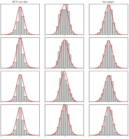
large d is likely to be normally distributed. One way to verify this is empirically, as we show in Figures 1-3 which contrast the histogram with a fitted normal pdf for text, digit images, and face images data. For these data sets the dimensionality d is sufficiently high to provide a nearly normal f_θ(X)_|Y . For example, in the case of text documents (Xi is the relative number of times word i appeared in the document) d corresponds to the vocabulary size which is typically a large number in the range 103₋105. Similarly, in the case of image classification (Xi denotes the brightness of the i-pixel) the dimensionality is on the order of 102₋104.

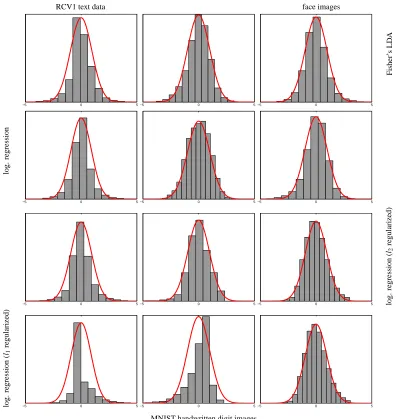
Figures 1-3 show that in these cases of text and image data f_θ(X)_|Y is approximately normal

for both randomly drawnθvectors (Figure 1) and forθrepresenting estimated classifiers (Figures 2

and 3). A caveat in this case is that normality may not hold whenθis sparse, as may happen for

example for L1regularized models (last row of Figure 2).

RCV1 text data face images

−5 0 5 −5 0 5 −5 0 5

−5 0 5 −5 0 5 −5 0 5

−5 0 5 −5 0 5 −5 0 5

−5 0 5 −5 0 5 −5 0 5

MNIST handwritten digit images

Figure 1: Centered histograms of f_θ(X)_|{Y =1_}overlayed with the pdf of a fitted Gaussian for

randomly drawnθvectors (θi∼U(−1/2,1/2)). The columns represent data sets (RCV1 text data, Lewis et al., 2004, MNIST digit images, and face images, Pham et al., 2002) and the rows represent multiple random draws. For uniformity we subtracted the empirical mean and divided by the empirical standard deviation. The twelve panels show that even in moderate dimensionality (RCV1: 1000 top words, MNIST digits: 784 pixels, face

images: 400 pixels) the assumption that f_θ(X)_|Y is normal holds often for randomly

RCV1 text data face images

−5 0 5 −5 0 5 −5 0 5

F

is

h

er

’s

L

D

A

lo

g

.

re

g

re

ss

io

n

−5 0 5 −5 0 5 −5 0 5

−5 0 5 −5 0 5 −5 0 5 lo

g

.

re

g

re

ss

io

n

(l2

re

g

u

la

ri

ze

d

)

lo

g

.

re

g

re

ss

io

n

(l1

re

g

u

la

ri

ze

d

)

−5 0 5 −5 0 5 −5 0 5

MNIST handwritten digit images

Figure 2: Centered histograms of f_θ(X)_|{Y =1_}overlayed with the pdf of a fitted Gaussian for

multipleθvectors (four rows: Fisher’s LDA, logistic regression, l2 regularized logistic

regression, and l1 regularized logistic regression-all regularization parameters were

se-lected by cross validation) and data sets (columns: RCV1 text data, Lewis et al., 2004, MNIST digit images, and face images, Pham et al., 2002). For uniformity we subtracted the empirical mean and divided by the empirical standard deviation. The twelve panels show that even in moderate dimensionality (RCV1: 1000 top words, MNIST digits: 784 pixels, face images: 400 pixels) the assumption that f_θ(X)_|Y is normal holds well for

fit-tedθvalues (except perhaps for L1regularization in the last row which promotes sparse

USPS ISOLET

−5 0 5 −5 0 5 −5 0 5

F

is

h

er

’s

L

D

A

lo

g

.

re

g

re

ss

io

n

−5 0 5 −5 0 5 −5 0 5

−5 0 5 −5 0 5 −5 0 5 lo

g

.

re

g

re

ss

io

n

(l2

re

g

u

la

ri

ze

d

)

lo

g

.

re

g

re

ss

io

n

(l1

re

g

u

la

ri

ze

d

)

−5 0 5 −5 0 5 −5 0 5

Arcene

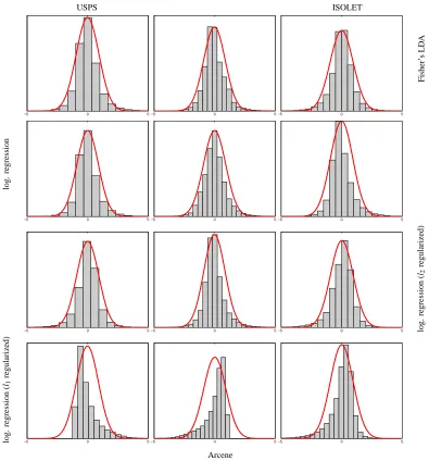
Figure 3: Centered histograms of fθ(X)_|{Y =1_}overlayed with the pdf of a fitted Gaussian for

multipleθvectors (four rows: Fisher’s LDA, logistic regression, l2 regularized logistic

regression, and l1 regularized logistic regression-all regularization parameters were

se-lected by cross validation) and data sets (columns: USPS Handwritten Digits, Arcene data set, and ISOLET). For uniformity we subtracted the empirical mean and divided by the empirical standard deviation. The twelve panels further confirm that the assumption that fθ(X)_|Y is normal holds well for fittedθvalues (except perhaps for L1regularization in the last row which promotes sparseθ) for various data sets.

Proposition 1 (de-Moivre) If Zi,i ∈ N are iid with expectation µ and variance σ2 and ¯

Zd=d−1∑di=1Zithen we have the following convergence in distribution

√

As a result, the quantity∑d_i=1Zi(which is a linear transformation of√d(_Zd¯ _{−µ)/σ) is approximately} normal for large d. This relatively restricted theorem is unlikely to hold in most practical cases as the data dimensions are often not iid.

A more general CLT does not require the summands Zito be identically distributed.

Proposition 2 (Lindberg) For Zi,i∈Nindependent with expectation µi and varianceσ2i, and de-noting s2_d=∑d

i=1σ2i, we have the following convergence in distribution as d→∞ s−_d1

d

∑

i=1

(Zi−µi) N(0,1)

if the following condition holds for everyε>0

lim d→∞s

−2

d d

∑

i=1

E(Zi₋µi)21_{|Xi−µi|>εsd}=0. (13) This CLT is more general as it only requires that the data dimensions be independent. The condition (13) is relatively mild and specifies that contributions of each of the Zito the variance sdshould not dominate it. Nevertheless, the Lindberg CLT is still inapplicable for dependent data dimensions.

More general CLTs replace the condition that Zi,i∈Nbe independent with the notion of m(k) -dependence.

Definition 3 The random variables Zi,i∈Nare said to be m(k)-dependent if whenever s−r>m(k) the two sets_{Z1, . . . ,Zr},{Zs, . . . ,Zk}are independent.

An early CLT for m(k)-dependent RVs was provided by Hoeffding and Robbins (1948). Below is a

slightly weakened version of the CLT, as proved in Berk (1973).

Proposition 4 (Berk) For each k_∈N_{let d(k)and m(k)be increasing sequences and suppose that} Z₁(k), . . . ,Z_d(k₍)_k)is an m(k)-dependent sequence of random variables. If

1. E_|Z_i(k)_|2_≤M for all i and k,

2. Var(Z_i(₊k)₁+. . .+Z(_jk))_≤(j₋i)K for all i,j,k,

3. limk_→∞Var(Z₁(k)+. . .+Z_d(k₍)_k))/d(k)exists and is non-zero, and 4. limk_→∞m2(k)/d(k) =0

then ∑ d(k) i=1Z

(k) i

√

d(k) is asymptotically normal as k→∞.

Proposition 4 states that under mild conditions the sum of m(k)-dependent RVs is asymptotically normal. If m(k)is a constant, that is, m(k) =m, m(k)-dependence implies that a Zimay only depend on its neighboring dimensions (in the sense of Definition 3). Intuitively, dimensions whose indices are far removed from each other are independent. The full power of Proposition 4 is invoked when

m(k)grows with k relaxing the independence restriction as the dimensionality grows. Intuitively,

the dependency of the summands is not fixed to a certain order, but it cannot grow too rapidly.

A more realistic variation of m(k)dependence where the dependency of each variable is

Definition 5 A graph

G

V

E

V

E

Proposition 6 (Rinott) Let Z1, . . . ,Znbe random variables having a dependency graph whose max-imal degree is strictly less than D, satisfying |Zi−EZi| ≤B a.s., ∀i, E(∑n

i=1Zi) = λ and Var(∑n_i=1Zi) =σ2_{>0, Then for any w∈R,}

P

∑n

i=1Zi−λ

σ ≤w

−Φ(w)

≤

1

σ

1

√

2πDB+16

n

σ2

1/2

D3/2B2+10 n

σ2

D2B3

whereΦ(w)is the CDF corresponding to a N(0,1) distribution.

The above theorem states a stronger result than convergence in distribution to a Gaussian in that it states a uniform rate of convergence of the CDF. Such results are known in the literature as Berry

Essen bounds (Davidson, 1994). When D and B are bounded andVar(∑n

i=1Zi) =O(n) it yields a CLT with an optimal convergence rate of n−1/2.

The question of whether the above CLTs apply in practice is a delicate one. For text one can argue that the appearance of a word depends on some words but is independent of other words. Similarly for images it is plausible to say that the brightness of a pixel is independent of pixels that are spatially far removed from it. In practice one needs to verify the normality assumption

empirically, which is simple to do by comparing the empirical histogram of f_θ(X)with that of a

fitted mixture of Gaussians. As the figures above indicate this holds for text and image data for

some values ofθ, assuming it is not sparse. Also, it is worth mentioning that one dimensional CLTs

kick in relatively early perhaps at 50 or 100 dimensions. Even when the high dimensional data lie on a lower dimensional manifold whose dimensionality is on the order of 100 dimensions, the CLT still applies to some extent (see histogram plots).

2.2 Unsupervised Consistency of ˆRn(θ)

We start with proving identifiability of the maximum likelihood estimator (MLE) for a mixture of two Gaussians with known ordering of mixture proportions. Invoking classical consistency results in

conjunction with identifiability we show consistency of the MLE estimator for(µ,σ)parameterizing

the distribution of f_θ(X)_|Y . As a result consistency of the estimator ˆRn(θ)follows.

Definition 7 A parametric family_{p_α:α_∈A_}is identifiable when p_α(x) =p_α′(x),∀x impliesα= α′_.

Proposition 8 Assuming known label marginals with p(Y =1)₆=p(Y=₋1)the Gaussian mixture family

pµ,σ(x) =p(y=1)N(x ; µ1,σ21) +p(y=−1)N(x ; µ−1,σ2₋1) is identifiable.

Proof It can be shown that the family of Gaussian mixture model with no apriori information about

assuming with no loss of generality that p(y=1)> p(y=₋1). The alternative case p(y=1)<

p(y=₋1)may be handled in the same manner. Using the result of Teicher (1963) we have that if

pµ,σ(x) =pµ′_,σ′(x)for all x, then(p(y),µ,σ) = (p(y),µ′,σ′)up to a permutation of the labels. Since

permuting the labels violates our assumption p(y=1)> p(y=₋1) we establish(µ,σ) = (µ′,σ′₎

proving identifiability.

The assumption that p(y)is known is not entirely crucial. It may be relaxed by assuming that it

is known whether p(Y =1)>p(Y =₋1)or p(Y =1)<p(Y =₋1). Proving Proposition 8 under this much weaker assumption follows identical lines.

Proposition 9 Under the assumptions of Proposition 8 the MLE estimates for (µ,σ) = (µ1,µ−1,σ1,σ−1)

(ˆµ(n),σˆ(n)) =arg max µ,σ

ℓn(µ,σ),

ℓn(µ,σ) = n

∑

i=1

log

∑

y(i)_∈{−1,+1}

p(y(i))pµy,σy(fθ(X (i)₎

|y(i)).

are consistent, that is,(ˆµ(₁n),ˆµ₋(n₁),σˆ₁(n),σˆ(₋n₁))converge as n_→∞to the true parameter values with probability 1.

Proof Denoting p_η(z) =∑_yp(y)pµy,σy(z|y) with η= (µ,σ) we note that pη is identifiable (see Proposition 8) inηand the available samples z(i)= f_θ(X(i))are iid samples from pη(z). We there-fore use standard statistics theory which indicates that the MLE for identifiable parametric model is strongly consistent (Ferguson, 1996, Chapter 17).

Proposition 10 Under the assumptions of Proposition 8 and assuming the loss

L

ˆ

Rn(θ) =

∑

p(y)

Z

R

p

ˆµ(yn),σˆ(yn)(fθ(X) =α|y)

L

P

lim n

ˆ

Rn(θ) =R(θ)=1.

Proof The plug-in risk estimate ˆRn in (14) is a continuous function (when L is given by (2), (3) or (4)) of ˆµ₁(n),ˆµ₋(n₁),σˆ(₁n),σˆ(₋n₁) (note that µy andσy are functions of θ), which we denote ˆRn(θ) = h(ˆµ(₁n),ˆµ(₋n₁),σˆ(₁n),σˆ(₋n₁)).

Using Proposition 9 we have that

lim n_→∞(ˆµ

(n)

1 ,ˆµ

(n)

−1,σˆ

(n)

1 ,σˆ

(n)

−1) = (µ true

1 ,µtrue−1,σtrue1 ,σtrue−1) with probability 1. Since continuous functions preserve limits we have

lim n_→∞h(ˆµ

(n)

1 ,ˆµ

(n)

−1,σˆ

(n)

1 ,σˆ

(n)

−1) =h(µtrue1 ,µ−true1,σtrue1 ,σtrue−1)

2.3 Unsupervised Consistency of arg min ˆRn(θ)

The convergence above ˆRn(θ)_→R(θ) is pointwise inθ. If the stronger concept of uniform

con-vergence is assumed overθ_∈Θ we obtain consistency of arg min_θRnˆ (θ). This surprising result

indicates that in some cases it is possible to retrieve the expected risk minimizer (and therefore the Bayes classifier in the case of the hinge loss, log-loss and exp-loss) using only unlabeled data. We show this uniform convergence using a modification of Wald’s classical MLE consistency result (Ferguson, 1996, Chapter 17).

Denoting

pη(z) =

∑

y_∈{−1,+1_}

p(y)pµy,σy(f(X) =z|y), η= (µ1,µ−1,σ1,σ−1)

we first show that the MLE converges to the true parameter value ˆηn→η0 uniformly. Uniform

convergence of the risk estimator ˆRn(θ)follows. Since changingθ_∈Θresults in a differentη_∈E

we can state the uniform convergence inθ_∈Θor alternatively inη_∈E.

Proposition 11 Letθtake values inΘfor whichη∈E for some compact set E. Then assuming the conditions in Proposition 10 the convergence of the MLE to the true value ˆηn→η0 is uniform in

η0∈E (or alternativelyθ∈Θ).

Proof We start by making the following notation

U(z,η,η0) =log pη(z)−log pη0(z),

α(η,η0) =Epη0U(z,η,η0) =−D(pη0,pη)≤0

with the latter quantity being non-positive and 0 iffη=η0(due to Shannon’s inequality and

identi-fiability of p_η).

Forρ>0 we define the compact set Sη0,ρ={η∈E :kη−η0k ≥ρ}. Sinceα(η,η0)is continu-ous it achieves its maximum (with respect toη) on S_η0,ρdenoted byδρ(η0) =maxη∈Sη0,ρα(η,η0)<

0 which is negative sinceα(η,η0) =0 iffη=η0. Furthermore, note thatδρ(η0)is itself continuous inη0∈E and since E is compact it achieves its maximum

δ=max

η0∈Eδρ(η0) =η0max∈E ηmax∈Sη0,ρ

α(η,η0)<0 which is negative for the same reason.

Invoking the uniform strong law of large numbers (Ferguson, 1996, Chapter 16) we have n−1∑n_i=1U(z(i),η,η0)→α(η,η0) uniformly over (η,η0)∈E2. Consequentially, there exists N such that for n>N (with probability 1)

sup

η0∈E sup

η∈Sη0,ρ

1 n

n

∑

i=1

U(z(i),η,η0)<δ/2<0.

But since n−1∑n_i=1U(z(i),η,η0)→0 forη=η0it follows that the MLE ˆ

ηn= max

η∈E 1 n

n

∑

i=1

U(z(i),η,η0)

Proposition 12 Assuming that X,Θare bounded in addition to the assumptions of Proposition 11 the convergence ˆRn(θ)_→R(θ)is uniform inθ_∈Θ.

Proof Since X,Θare bounded the margin value fθ(X)is bounded with probability 1. As a result the loss function is bounded in absolute value by a constant C. We also note that a mixture of two Gaussian model (with known mixing proportions) is Lipschitz continuous in its parameters

_y∈{−

∑

p(y)p

ˆµy(n),σˆy(n)(z)−

∑

p(y)pµtrue y ,σtruey (z)

≤t(z)_· (ˆµ

(n)

1 ,ˆµ

(n)

−1,σˆ

(n)

1 ,σˆ

(n)

−1)−(µtrue1 ,µ₋true1,σtrue1 ,σtrue₋1)

which may be verified by noting that the partial derivatives of pη(z) =∑_yp(y)pµy,σy(z|y)

∂pη(z) ∂ˆµ(₁n)

= p(y=1)(z−ˆµ (n)

1 )

(2π)1/2σ_ˆ(n)3 1

e

−(z−ˆµ

(n) 1 )2 2 ˆσ(₁n)3 _,

∂p_η(z) ∂ˆµ(₋n₁)

= p(y=−1)(z−ˆµ (n)

−1)

(2π)1/2σ_ˆ(n)3

−1

e

−(z−ˆµ

(n)

−1)2 2 ˆσ(₋n₁)3 _,

∂p_η(z) ∂σˆ(₁n) =−

p(y=1)(z₋ˆµ(₁n))2

(2π)3/2σ_ˆ(n)6 1

e

−(z−ˆµ

(n) 1 )2 2 ˆσ(₁n)2 _,

∂p_η(z) ∂σˆ(₋n₁)

=₋p(y=−1)(z−ˆµ (n)

−1)2

(2π)3/2σ_ˆ(n)6

−1

e

−(z−ˆµ

(n)

−1)2 2 ˆσ(₋n₁)2

are bounded for a compact E. These observations, together with Proposition 11 lead to

|_Rnˆ ₍θ_)−R(θ_{)| ≤}

∑

p(y)

Z

p_ˆµ(_yn)_,σ_ˆ(_yn)(fθ(X) =α)−pµtruey ,σtruey (fθ(X) =α)

|

L

≤C

Z

∑

y∈{−1,+1}

p(y)p

ˆµy(n),σˆy(n)(α)−

∑

p(y)pµtrue

y ,σtruey (α)

dα

≤C_k(ˆµ(₁n),ˆµ₋(n₁),σˆ(₁n),σˆ₋(n₁))₋(µtrue₁ ,µ₋true₁,σtrue₁ ,σtrue₋₁)_k

Z b

a t(z)dz

≤C′_k(ˆµ(₁n),ˆµ(₋n₁),σˆ₁(n),σˆ(₋n₁))₋(µtrue₁ ,µtrue₋₁,σtrue

1 ,σtrue−1)k →0

uniformly overθ_∈Θ.

Proposition 13 Under the assumptions of Proposition 12

P

lim

n→∞arg min_θ∈Θ Rˆn(θ) =arg min_θ∈Θ R(θ)

Proof We denote t∗=arg min R(θ), tn=arg min ˆRn(θ). Since ˆRn(θ)_→R(θ)uniformly, for each

ε>0 there exists N such that for all n>N,_|Rnˆ (θ)₋R(θ)_|<ε.

Let S=_{θ:_kθ₋t∗_{k ≥}ε_}and min_θ∈SR(θ)>R(t∗)(S is compact and thus R achieves its min-imum on it). There exists N′ such that for all n>N′ andθ∈S, ˆRn(θ)_≥R(t∗) +ε. On the other hand, ˆRn(t∗)_→R(t∗)which together with the previous statement implies that there exists N′′such that for n>N′′, ˆRn(t∗)<Rˆn(θ)for allθ∈S. We thus conclude that for n>N′′, tn6∈S. Since we showed that for each ε>0 there exists N such that for all n>N we have _ktn−t∗k ≤ε, tn→t∗ which concludes the proof.

2.4 Asymptotic Variance

In addition to consistency, it is useful to characterize the accuracy of our estimator ˆRn(θ) as a

function of p(y),µ,σ. We do so by computing the asymptotic variance of the estimator which

equals the inverse Fisher information

√

n(ηˆmle_{n −}η0) N(0,I−1(ηtrue))

and analyzing its dependency on the model parameters. We first derive the asymptotic variance of MLE for mixture of Gaussians (we denote belowη= (η1,η2),ηi= (µi,σi))

pη(z) =p(Y =1)N(z; µ1,σ2₁) +p(Y =₋1)N(z; µ₋1,σ2₋1)

=p1pη1(z) +p₋1pη−1(z).

The elements of 4_×4 information matrix I(η)

I(ηi,ηj) =E

∂

log p_η(z) ∂ηi

∂log p_η(z) ∂ηj

may be computed using the following derivatives

∂log p_η(z) ∂µi

= pi σi

z₋µi

σi

p_ηi(z) p_η(z), ∂log pη(z)

∂σ2 i

= pi

2σi

z₋µi

σi

2

−1

!

pηi(z) p_η(z)

for i=1,₋1. Using the method of Behboodian (1972) we obtain

I(µi,µj) = pipj

σiσj M11

p_ηi(z),pηi(z)

,

I(µ1,σ2i) = p1pi 2σ1σ2i

h

M12

p_ηi(z),pηi(z)

−M10

p_η1(z),p_ηi(z)

i

,

I(µ₋1,σ2i) = p₋1pi 2σ₋1σ2i

h

M21

pηi(z),pη−1(z)

−M01

pηi(z),pη−1(z)

i

,

I(σ2 i,σ2i) =

p4_i 4σ4

i

h

M00

p_ηi(z),p_ηi(z)₋2M11

p_ηi(z),p_ηi(z)+M22

p_ηi(z),p_ηi(z)i,

I(σ2₁,σ2₋₁) = p1p−1

4σ2₁σ2₋₁

h

M00

pη1(z),pη−1(z)

−M20

pη1(z),pη−1(z)

−M02

p_η1(z),p_η−1(z)+M22

where

Mm,n

p_ηi(z),p_ηj(z)=

Z _∞

−∞

z₋µi

σi

m

z₋µj

σj

n _p

ηi(z)pηj(z) pη(z) dx.

In some cases it is more instructive to consider the asymptotic variance of the risk estimator ˆ

Rn(θ)rather than that of the parameter estimate forη= (µ,σ). This could be computed using the delta method and the above Fisher information matrix

√

n(_Rˆ_{n(θ)−R(θ)) N(0,∇h(η}true₎T_I−1_(ηtrue_)∇h(ηtrue₎₎

where ∇h is the gradient vector of the mapping R(θ) =h(η). For example, in the case of the

exponential loss (2) we get

h(η) =p(Y =1)σ1

√

2 exp

(µ1−1)2

2 −

µ2₁ 2σ2₁

+p(Y =₋1)σ₋1

√

2 exp

(µ

−1−1)2

2 −

µ2₋₁ 2σ2₋₁

,

∂h(η)

∂µ1 =

√

2P(Y=1)(µ1(σ2

1−1)−σ21)

σ1

exp

(µ1₋1)2

2 −

µ2₁ 2σ2₁

,

∂h(η) ∂µ₋1

= √

2P(Y=₋1)(µ₋1(σ2₋₁−1) +σ2₋₁)

σ₋1

exp (µ−1+1) 2

2 −

µ2₋₁ 2σ2₋₁

!

,

∂h(η) ∂σ2

1

=P(Y =1)(µ

2 1+σ21)

√

2σ1

(µ₁−1)2

2 −

µ2 1 2σ2

1

,

∂h(η) ∂σ2

−1

=P(Y =−1)(µ

2

−1+σ2−1)

√

2σ₋1

(µ

−1+1)2

2 −

µ2₋₁ 2σ2

−1

.

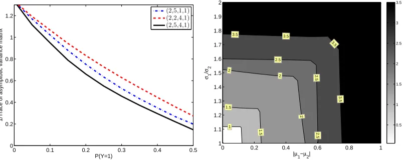
Figure 4 plots the asymptotic accuracy of ˆRn(θ) for log-loss. The left panel shows that the

accuracy of ˆRn increases with the imbalance of the marginal distribution p(Y). The right panel

shows that the accuracy of ˆRn increases with the difference between the means_|µ1₋µ₋1|and the

variancesσ1/σ2.

2.5 Multiclass Classification

Thus far, we have considered unsupervised risk estimation in binary classification. In this section we describe a multiclass extension based on standard extensions of the margin concept to multiclass classification. In this case the margin vector associated with the multiclass classifier

ˆ

Y =arg max

k=1,...,K

f_θk(X), X,θk∈Rd

is fθ(X) = (fθ1(X), . . . ,fθK(X)). Following our discussion of the binary case, f_θk(X)|Y , k=1, . . . ,K is assumed to be normally distributed with parameters that are estimated by maximizing the like-lihood of a Gaussian mixture model. We thus have K Gaussian mixture models, each one with K mixture components. The estimated parameters are plugged-in as before into the multiclass risk

0 0.1 0.2 0.3 0.4 0.5 0

0.2 0.4 0.6 0.8 1 1.2

P(Y=1)

1/Trace of asymptotic variance matrix

(2,5,1,1) (2,2,4,1) (2,5,4,1)

1 1.5

1.5

2

2

2

2.5

2.5

2.5

3.5

3.5

3.5 3.5

|µ₁−µ₂|

σ1

/

σ2

0 0.2 0.4 0.6 0.8 1

1 1.1 1.2 1.3 1.4 1.5 1.6 1.7 1.8 1.9 2

0.5 1 1.5 2 2.5 3 3.5

Figure 4: Left panel: asymptotic accuracy (inverse of trace of asymptotic variance) of ˆRn(θ) for

logloss as a function of the imbalance of the class marginal p(Y). The accuracy increases with the class imbalance as it is easier to separate the two mixture components. Right panel: asymptotic accuracy (inverse of trace of asymptotic variance) as a function of the difference between the means _|µ1−µ−1| and the variances σ1/σ2. See text for more information.

where

L

L

∑

k6=Y

log(1+exp(₋f_θk(X))), (15)

L

∑

k6=Y

(1+f_θk(X))₊. (16)

Care should be taken when defining the loss function for the multi-class case, as a straight-forward extension from the binary case might render the framework inconsistent. We use the specific ex-tension which is proved to be consistent for various loss functions (including hinge-loss) by Tewari and Bartlett (2007). Since the MLE for a Gaussian mixture model with K components is consistent (assuming P(Y)is known and all probabilities P(Y =k),k=1, . . . ,K are distinct) the MLE estima-tor for f_θk(X)|Y =k′ are consistent. Furthermore, if the loss

L

3. Application 1: Estimating Risk in Transfer Learning

We consider applying our estimation framework in two ways. The first application, which we describe in this section, is estimating margin-based risks in transfer learning where classifiers are trained on one domain but tested on a somewhat different domain. The transfer learning assumption that labeled data exists for the training domain but not for the test domain motivates the use of our unsupervised risk estimation. The second application, which we describe in the next section, is more ambitious. It is concerned with training classifiers without labeled data whatsoever.

In evaluating our framework we consider both synthetic and real-world data. In the synthetic

10000 2500 5000 7500 10000 0.001

0.002 0.003 0.004 0.005 0.006 0.007 0.008 0.009 0.01

acc=0.6 acc=0.7 acc=0.8 acc=0.9

10000 2500 5000 7500 10000

0.002 0.004 0.006 0.008 0.01 0.012

acc=0.6 acc=0.7 acc=0.8 acc=0.9

10000 2500 5000 7500 10000

0.002 0.004 0.006 0.008 0.01 0.012 0.014 0.016 0.018 0.02

P(y=1)=0.65 P(y=1)=0.75 P(y=1)=0.85 P(y=1)=0.95

10000 2500 5000 7500 10000

0.005 0.01 0.015 0.02 0.025

P(y=1)=0.65 P(y=1)=0.75 P(y=1)=0.85 P(y=1)=0.95

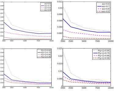
Figure 5: The relative accuracy of ˆRn (measured by _|Rnˆ (θ)₋Rn(θ)_|/Rn(θ)) as a function of n, classifier accuracy (acc) and the label marginal p(Y) (left: logloss, right: hinge-loss).

The estimation error nicely decreases with n (approaching 1% at n=1000 and decaying

further). It also decreases with the accuracy of the classifier (top) and non-uniformity of p(Y)(bottom) in accordance with the theory of Section 2.4.

X|{Y =₋1}with independent dimensions and prescribed p(Y) and classification accuracy. This

controlled setting allows us to examine the accuracy of the risk estimator as a function of n, p(Y), and the classifier accuracy.

Figure 5 shows that the relative error of ˆRn(θ)(measured by|_Rnˆ _{(θ)−Rn(θ)|/Rn(θ)) in} estimat-ing the logloss (left) and hestimat-inge loss (right). The curves decrease with n and achieve accuracy of

greater than 99% for n>1000. In accordance with the theoretical results in Section 2.4 the

fig-ure shows that the estimation error decreases as the classifiers become more accurate and as p(Y)

becomes less uniform. We found these trends to hold in other experiments as well. In the case of exponential loss, however, the estimator performed substantially worse across the board, in some cases with an absolute error of as high as 10. This is likely due to the exponential dependency of the loss on Y fθ(X)which makes it very sensitive to outliers.

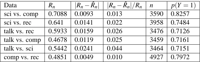
Data Rn _|Rn₋Rnˆ _{| |}Rn₋Rnˆ _|/Rn n p(Y =1)

sci vs. comp 0.7088 0.0093 0.013 3590 0.8257

sci vs. rec 0.641 0.0141 0.022 3958 0.7484

talk vs. rec 0.5933 0.0159 0.026 3476 0.7126

talk vs. comp 0.4678 0.0119 0.025 3459 0.7161

talk vs. sci 0.5442 0.0241 0.044 3464 0.7151

comp vs. rec 0.4851 0.0049 0.010 4927 0.7972

Table 1: Error in estimating logloss for logistic regression classifiers trained on one 20-newsgroup classification task and tested on another. We followed the transfer learning setup described by Dai et al. (2007) which may be referred to for more detail. The train and testing sets contained samples from two top categories in the topic hierarchy but with different subcat-egory proportions. The first column indicates the top catsubcat-egory classification task and the second indicates the empirical log-loss Rncalculated using the true labels of the testing set (5). The third and forth columns indicate the absolute and relative errors of ˆRn. The fifth and sixth columns indicate the train set size and the label marginal distribution.

data has a hierarchical class taxonomy and the transfer learning problem is defined at the top-level categories. We split the data based on subcategories such that the training and test sets contain data sampled from different subcategories within the same top-level category. Hence, the training and test distributions differ. We trained a logistic regression classifier on the training set and estimate its risk on the test set of a different distribution. Our unsupervised risk estimator was quite effective in estimating the risk with relative accuracy greater than 96% and absolute error less than 0.02.

4. Application 2: Unsupervised Learning of Classifiers

Our second application is a very ambitious one: training classifiers using unlabeled data by

min-imizing the unsupervised risk estimate ˆθn =arg min ˆRn(θ). We evaluate the performance of the

learned classifier ˆθnbased on three quantities: (i) the unsupervised risk estimate ˆRn(θˆn), (ii) the su-pervised risk estimate Rn(θˆn), and (iii) its classification error rate. We also compare the performance of ˆθn=arg min ˆRn(θ)with that of its supervised analog arg min Rn(θ).

We compute ˆθn=arg min ˆRn(θ) using two algorithms (see Algorithms 1-2) that start with an

initialθ(0) and iteratively construct a sequence of classifiersθ(1), . . . ,θ(T) _{which steadily decrease}

ˆ

Rn. Algorithm 1 adopts a gradient descent-based optimization. At each iteration t, it approximates the gradient vector∇Rnˆ (θ(t)_{)numerically using a finite difference approximation (17). We}

com-pute the integral in the loss function estimator using numeric integration. Since the integral is one dimensional a variety of numeric methods may be used with high accuracy and fast computation. Algorithm 2 proceeds by constructing a grid search along every dimension ofθ(t)and set[θ(t)_]

ito

the grid value that minimizes ˆRn (iteratively optimize one dimension at a time). This amounts to

Although we focus on unsupervised training of logistic regression (minimizing unsupervised logloss estimate), the same techniques may be generalized to train other margin-based classifiers such as SVM by minimizing the unsupervised hinge-loss estimate.

Algorithm 1 Unsupervised Gradient Descent

Input: X(1), . . . ,X(n)_∈Rd_{, p(Y), step size}α Initialize t =0,θ(t)=θ0_∈Rd

repeat

Compute f_θ(t)(X(j)) =hθ(t),X(j)i ∀j=1, . . . ,n

Estimate(ˆµ1,ˆµ₋1,σˆ1,σˆ₋1)by maximizing (11)

for i=1 to d do

Plug-in the estimates into (14) to approximate

∂_Rnˆ ₍θ(t)₎

∂θi

=Rnˆ (θ

(t)_{+hiei)−Rnˆ (θ}(t)_−hiei)

2hi

(ei is an all zero vector except for[ei]i=1) (17)

end for

Form∇Rnˆ (θ(t)_{) = (}∂Rˆn(θ(t))

∂θ(t) 1

, . . . ,∂Rˆn(θ(t))

∂θ(t) d

)

Updateθ(t+1)=θ(t)_−α∇Rˆ

n(θ(t)), t=t+1

until convergence

Output: linear classifierθfinal=θ(t)

Algorithm 2 Unsupervised Grid Search

Input: X(1), . . . ,X(n)∈Rd_{, p}(Y), grid-sizeτ Initializeθi∼Uniform(−2,2)for all i

repeat

for i=1 to d do

Constructτpoints grid in the range[θi−4τ,θi+4τ]

Compute the risk estimate (14) where all dimensions ofθ(t)are fixed except for[θ(t)_]

iwhich

is evaluated at each grid point. Set[θ(t+1)_]

ito the grid value that minimized (14)

end for

until convergence

Output: linear classifierθfinal=θ

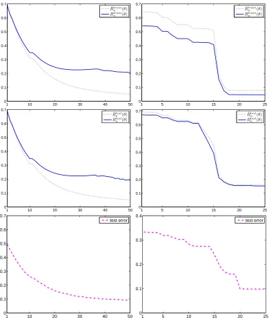
Figures 6-7 display ˆRn(θˆn), Rn(θˆn)and error-rate(θˆn)on the training and testing sets as on two real world data sets: RCV1 (text documents) and MNIST (handwritten digit images) data sets. In the case of RCV1 we discarded all but the most frequent 504 words (after stop-word removal) and represented documents using their tfidf scores. We experimented on the binary classification task of distinguishing the top category (positive) from the next 4 top categories (negative) which resulted in p(y=1) =0.3 and n=199328. 70% of the data was chosen as a (unlabeled) training set and the

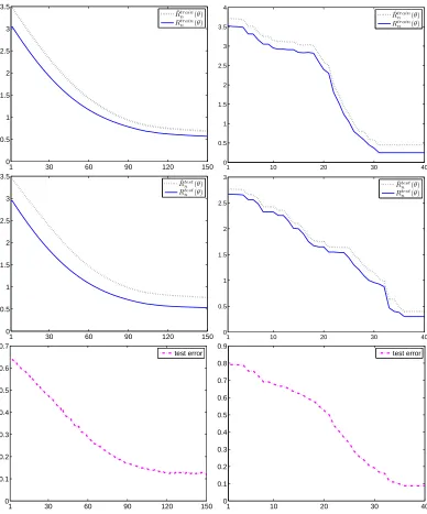
pixels to have 0 mean and unit variance. Our classification task was to distinguish images of the digit one (positive) from the digit 2 (negative) resulting in 14867 samples and p(Y=1) =0.53. We randomly choose 70% of the data as a training set and kept the rest as a testing set.

Figures 6-7 indicate that minimizing the unsupervised logloss estimate is quite effective in learning an accurate classifier without labels. Both the unsupervised and supervised risk estimates

ˆ

Rn(θˆn), Rn(θˆn)decay nicely when computed over the train set as well as the test set. Also interesting is the decay of the error rate. For comparison purposes supervised logistic regression with the same n achieved only slightly better test set error rate: 0.05 on RCV1 (instead of 0.1) and 0.07 or MNIST (instead of 0.1).

In another experiment we examined the proposed approach on several different data sets and compared the classification performance with a supervised baseline (logistic regression) and Gaus-sian mixture modeling (GMM) clustering with known label proportions in the original data space

(Table 2). The comparison was made under the same experimental setting (n, p(Y)) for all three

approaches. We used data sets from UCI machine learning repository (Frank and Asuncion, 2010) and from previously cited sources, unless otherwise noted. The following tasks were considered for each data set.

• RCV1: top category versus next 4 categories

• MNIST: Digit 1 versus Digit 2

• 20 newsgroups: Comp category versus Recreation category

• USPS1: Digit 2 versus Digit 5

• Umist1: Male face (16 subjects) versus Female faces (4 subjects) with image resolution

re-duced to 40_×40

• Arcene: Cancer versus Normal

• Isolet: Vowels versus Consonants

• Dexter: Documents about corporate acquisitions versus rest

• Secom: Semiconductor manufacturing defects versus good items

• Pham faces: Face versus Non-face images

• CMU pie face2: male (30 subjects) vs female (17 subjects)

• Madelon3: It consists of data points (artificially generated) grouped in 32 clusters placed on

the vertices of a five dimensional hypercube and randomly labeled +1 or -1, corrupted with features that are not useful for classification.

1. Data set can be found athttp://www.cs.nyu.edu/˜roweis/data.html.

2. Data set can be found athttp://www.zjucadcg.cn/dengcai/Data/FaceData.html.

3. Data set can be found at http://archive.ics.uci.edu/ml/machine-learning-databases/madelon/

1 10 20 30 40 50 0

0.1 0.2 0.3 0.4 0.5 0.6 0.7

ˆ

Rtrain

n (θ)

Rtrain

n (θ)

1 5 10 15 20 25

0 0.1 0.2 0.3 0.4 0.5 0.6 0.7

ˆ

Rtrain

n (θ)

Rtrain

n (θ)

1 10 20 30 40 50

0 0.1 0.2 0.3 0.4 0.5 0.6 0.7

ˆ Rtest

n (θ)

Rtest

n (θ)

1 5 10 15 20 25

0 0.1 0.2 0.3 0.4 0.5 0.6 0.7

ˆ Rtest

n (θ)

Rtest

n (θ)

1 10 20 30 40 50

0 0.1 0.2 0.3 0.4 0.5 0.6 0.7

test error

1 5 10 15 20 25

0 0.1 0.2 0.3 0.4

test error

Figure 6: Performance of unsupervised logistic regression classifier ˆθncomputed using Algorithm 1

(left) and Algorithm 2 (right) on the RCV1 data set. The top two rows show the decay of the two risk estimates ˆRn(θˆn), Rn(θˆn) as a function of the algorithm iterations. The

risk estimates of ˆθn were computed using the train set (top) and the test set (middle).

The bottom row displays the decay of the test set error rate of ˆθn as a function of the

algorithm iterations. The figure shows that the algorithm obtains a relatively accurate

classifier (testing set error rate 0.1, and ˆRn decaying similarly to Rn) without the use

1 30 60 90 120 150 0

0.5 1 1.5 2 2.5 3 3.5

ˆ

Rtrain

n (θ)

Rtrain

n (θ)

1 10 20 30 40

0 0.5 1 1.5 2 2.5 3 3.5 4

ˆ

Rtrain

n (θ)

Rtrain

n (θ)

1 30 60 90 120 150

0 0.5 1 1.5 2 2.5 3 3.5

ˆ Rtest

n (θ)

Rtest

n (θ)

1 10 20 30 40

0 0.5 1 1.5 2 2.5 3

ˆ Rtest

n (θ)

Rtest

n (θ)

1 30 60 90 120 150

0 0.1 0.2 0.3 0.4 0.5 0.6 0.7

test error

1 10 20 30 40

0 0.1 0.2 0.3 0.4 0.5 0.6 0.7 0.8 0.9

test error

Figure 7: Performance of unsupervised logistic regression classifier ˆθncomputed using Algorithm 1

(left) and Algorithm 2 (right) on the MNIST data set. The top two rows show the decay of the two risk estimates ˆRn(θˆn), Rn(θˆn) as a function of the algorithm iterations. The

risk estimates of ˆθn were computed using the train set (top) and the test set (middle).

The bottom row displays the decay of the test set error rate of ˆθn as a function of the

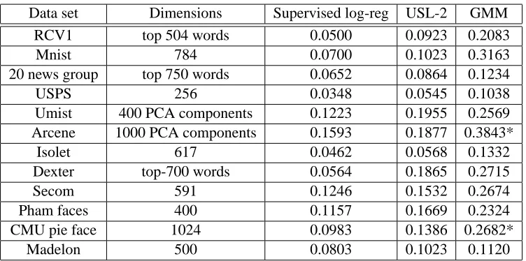
Data set Dimensions Supervised log-reg USL-2 GMM

RCV1 top 504 words 0.0500 0.0923 0.2083

Mnist 784 0.0700 0.1023 0.3163

20 news group top 750 words 0.0652 0.0864 0.1234

USPS 256 0.0348 0.0545 0.1038

Umist 400 PCA components 0.1223 0.1955 0.2569

Arcene 1000 PCA components 0.1593 0.1877 0.3843*

Isolet 617 0.0462 0.0568 0.1332

Dexter top-700 words 0.0564 0.1865 0.2715

Secom 591 0.1246 0.1532 0.2674

Pham faces 400 0.1157 0.1669 0.2324

CMU pie face 1024 0.0983 0.1386 0.2682*

Madelon 500 0.0803 0.1023 0.1120

Table 2: Comparison (test set error rate) between supervised logistic regression, Unsupervised lo-gistic regression and Gaussian mixture modeling in original data space. The unsupervised classifier performs better than the GMM clustering on the original space and compares well with its supervised counterpart on most data sets. See text for more details. The stars

represent GMM with covarianceσ2I due to the high dimensionality. In all other cases we

used a diagonal covariance matrix. Non-diagonal covariance matrix was impractical due to the high dimensionality.

Table 2 displays the test set error for the three methods on each data set. We note that our unsupervised approach achieves test set errors comparable to the supervised logistic regression in several data sets. The poor performance of the unsupervised technique on the Dexter data set is due to the fact that the data contains many irrelevant features. In fact it was engineered for a feature selection competition and has a sparse solution vector. In general our method significantly outperforms Gaussian mixture model clustering in the original feature space. A likely explanation is that (i) f_θ(X)_|Y is more likely to be normal than X_|Y and (ii) it is easier to estimate in one dimensional space rather than in a high dimensional space.

4.1 Inaccurate Specification of p(Y)

Our estimation framework assumes that the marginal p(Y)is known. In some cases we may only

have an inaccurate estimate of p(Y). It is instructive to consider how the performance of the learned classifier degrades with the inaccuracy of the assumed p(Y).

Figure 8 displays the performance of the learned classifier for RCV1 data as a function of the assumed value of p(Y =1)(correct value is p(Y =1) =0.3). We conclude that knowledge of p(Y)

0.1 0.2 0.3 0.4 0.5 0.6 0.7 0.8 0.9 0.1

0.2 0.3 0.4 0.5 0.6

|Rn(P(y)6=0.3)−R(nP(y)=0.3)|

test error

Figure 8: Performance of unsupervised classifier training on RCV1 data (top class vs. classes 2-5) for misspecified p(Y). The performance of the estimated classifier (in terms of training

set empirical logloss Rn(5) and test error rate measured using held-out labels) decreases

with the deviation between the assumed and true p(Y =1)(true p(Y =1) =0.3)). The

classifier performance is very good when the assumed p(Y) is close to the truth and

degrades gracefully when the assumed p(Y)is not too far from the truth.

4.2 Effect of Regularization and Dimensionality Reduction

In Figure 9 we examine the effect of regularization on the performance of the unsupervised classifier.

In this experiment we use the L1 regularization software available at http://www.cs.ubc.ca/

˜schmidtm/Software/L1General.html. Clearly, regularization helps in the supervised case. It

appears that in the USL case weak regularization may improve performance but not as drastically as

in the supervised case. Furthermore, the positive effect of L1regularization in the USL case appears

to be weaker than L2regularization (compare the left and right panels of Figure 9). One possible

reason is that the sparsity promoting nature of L1conflicts with the CLT assumption.

In Figure 10 we examine the effect of reducing the data dimensionality via PCA prior to training the unsupervised classifier. Specifically, the 256 dimensions USPS image data set was embedded in an increasingly lower dimensional space via PCA. For the original dimensionality of 256 or a slightly lower dimensionality the classification performance of the unsupervised classifier is com-parable to the supervised. Once the dimensions are reduced to less than 150 a significant perfor-mance gap appears. This is consistent with our observation above that for lower dimensions the CLT approximation is less accurate. The supervised classifier also degrades in performance as less dimensions are used but not as fast as the unsupervised classifier.

5. Related Work

0.1 0.2 0.3 0.4 0.5 0.6 0.7 0.8 0.9 1 0.04

0.045 0.05 0.055 0.06 0.065 0.07 0.075 0.08

Regularization parameter

Test error

l2−log reg l2−usl log reg

0.1 0.2 0.3 0.4 0.5 0.6 0.7 0.8 0.9 1

0.02 0.04 0.06 0.08 0.1 0.12 0.14 0.16 0.18

Regularization parameter

Test error

l1−log reg l1−usl log reg

Figure 9: Test set error rate versus regularization parameter (L2on the left panel and L1on the right panel) for supervised and unsupervised logistic regression on RCV1 data set.

2 10 50 100 125 150 200 256

0 0.05 0.1 0.15 0.2 0.25 0.3 0.35 0.4 0.45

Dimensions

Test error

usl log reg log reg

Figure 10: Test set error rate versus the amount of dimensions used (extracted via PCA) for super-vised and unsupersuper-vised logistic regression on USPS data set. The original dimensional-ity was 256.

a framework for training a classifier with no labeled samples, while approaches above still need labeled samples for classification.

Unsupervised approaches: The most recent related research approaches are by Quadrianto et al. (2009), Gomes et al. (2010), and Donmez et al. (2010). The work by Quadrianto et al. (2009) aims to estimate the labels of an unlabeled testing set using known label proportions of several sets of unlabeled observations. The key difference between their approach and ours is that they require separate training sets from different sampling distributions with different and known label marginals (one for each label). Our method assumes only a single data set with a known label marginal but on the other hand assumed the CLT approximation. Furthermore, as noted previously (see comment after Proposition 8), our analysis is in fact valid when only the order of label proportions is known, rather than the absolute values.

A different attempt at solving this problem is provided by Gomes et al. (2010) which focuses on discriminative clustering. This approach attempts to estimate a conditional probabilistic model in an unsupervised way by maximizing mutual information between the empirical input distribution and the label distribution. A key difference is the focus on probabilistic classifiers and in partic-ular logistic regression whereas our approach is based on empirical risk minimization which also includes SVM. Another key difference is that the work by Gomes et al. (2010) lacks consistency results which characterize when it works from a theoretical perspective. The approach by Donmez et al. (2010) focuses on estimating the error rate of a given stochastic classifier (not necessarily linear) without labels. It is similar in that it estimates the 0/1 risk rather than the margin based risk. However, it uses a different strategy and it replaces the CLT assumption with a symmetric noise assumption.

An important distinction between our work and the references above is that our work provides an estimate for the margin-based risk and therefore leads naturally to unsupervised versions of logistic regression and support vector machines. We also provide asymptotic analysis showing convergence of the resulting classifier to the optimal classifier (minimizer of (1)). Experimental results show that in practice the accuracy of the unsupervised classifier is on the same order (but slightly lower naturally) as its supervised analog.

6. Discussion

In this paper we developed a novel framework for estimating margin-based risks using only unla-beled data. We show that it performs well in practice on several different data sets. We derived a theoretical basis by casting it as a maximum likelihood problem for Gaussian mixture model followed by plug-in estimation.

Remarkably, the theory states that assuming normality of fθ(X)and a known p(Y)we are able

to estimate the risk R(θ)without a single labeled example. That is the risk estimate converges to the true risk as the number of unlabeled data increase. Moreover, using uniform convergence arguments it is possible to show that the proposed training algorithm converges to the optimal classifier as

n_→∞without any labeled data. The results in the paper are applicable only to linear classifiers,

our framework be extended to semi-supervised learning where a few labels do exist? Can it be extended to non-classification scenarios such as margin based regression or margin based structured prediction? When are the assumptions likely to hold and how can we make our framework even more resistant to deviations from them? These questions and others form new and exciting open research directions.

Acknowledgments

The authors thank the action editor and anonymous reviewers for their constructive comments, that not only helped at a conceptual level but also helped improve the presentation. In addition, we thank John Lafferty and Vladimir Koltchinskii for discussions and several insightful comments. This work was funded in part by NSF grant IIS-0906550.

References

J. Behboodian. Information matrix for a mixture of two normal distributions. Journal of Statistical Computation and Simulation, 1(4):295–314, 1972.

K. N. Berk. A central limit theorem for m-dependent random variables with unbounded m. The Annals of Probability, 1(2):352–354, 1973.

V. Castelli and T. M. Cover. On the exponential value of labeled samples. Pattern Recognition Letters, 16(1):105–111, 1995.

V. Castelli and T. M. Cover. The relative value of labeled and unlabeled samples in pattern recog-nition with an unknown mixing parameter. IEEE Transactions on Information Theory, 42(6): 2102–2117, 1996.

W. Dai, Q. Yang, G.-R. Xue, and Y. Yu. Boosting for transfer learning. In Proc. of International Conference on Machine Learning, 2007.

J. Davidson. Stochastic Limit Theory: An Introduction for Econometricians. Oxford University Press, USA, 1994.

P. Donmez, G. Lebanon, and K. Balasubramanian. Unsupervised supervised learning I: Estimating classification and regression error rates without labels. Journal of Machine Learning Research, 11(April):1323–1351, 2010.

T. S. Ferguson. A Course in Large Sample Theory. Chapman & Hall, 1996.

A. Frank and A. Asuncion. UCI machine learning repository. University of California, School of Information and Computer Science, Irvine, CA. Available at http://archive.ics.uci.edu/ml/, 2010.

R. Gomes, A. Krause, and P. Perona. Discriminative clustering by regularized information maxi-mization. In Advances in Neural Information Processing Systems 24, 2010.