http://www.sciencepublishinggroup.com/j/ijefm doi: 10.11648/j.ijefm.20170506.17
ISSN: 2326-9553 (Print); ISSN: 2326-9561 (Online)
The Factors Affecting Business Cycle Volatility Based on
Financial Market Size and Country Size Multiple-factor
Analysis
Shi Haoran
1, An Gang
21
Department of Industrial Engineering, School of Business Administration, Northeastern University, Shenyang, China
2
Department of International Economics and Trade, School of Business Administration, Northeastern University, Shenyang, China
Email address:
[email protected] (Shi Haoran), [email protected] (An Gang)
To cite this article:
Shi Haoran, An Gang. The Factors Affecting Business Cycle Volatility Based on Financial Market Size and Country Size Multiple-factor Analysis. International Journal of Economics, Finance and Management Sciences. Vol. 5, No. 6, 2017, pp. 321-326.
doi: 10.11648/j.ijefm.20170506.17
Received: November 15, 2017; Accepted: November 23, 2017; Published: December 28, 2017
Abstract:
The main purpose of this paper is to investigate the relationship between business cycle volatility and country size and financial markets size within certain countries, using annual data for a sample of some typical countries having advanced financial market and those of China over 2000-2015. Then analyze the significance level of explaining variables and the type of effect. The main result reflects that for OECD countries, the impacts of population and stock market are all highest level significant and most keep stable after authors filter out the fluctuations, but for China population is a stable significant factor, while the influences of stock market depend on the data processing method and even the plus-minus and the significance of the regression coefficient can change due to the filter process and authors will elaborate the inner economic principles it reveals.Keywords:
Business Cycle Volatility, Country Size, Financial Market Size, Panel Data Analyses1. Introduction
Why the authors would like to research on this project? In recent days, the chairman of CSRC Liu Shiyu has been emphasizing the importance of limiting IPO (Initially Public Offerings) for several times. These had of course reminded us of the necessity of controlling the financial markets sizes. As an aspect of it, authors would like to research the relationship between financial markets sizes and business cycle volatility. Furthermore, before writing this paper, Authors made a sketchy statistics. The statistics focus on a special period in last century during which “327 incident” and “810 incident” broke out. Both of them are due to blind expansion of financial market.
The authors take the GDP data from Chinese national, then authors did a fundamental statistic, finding that during 1990-2001 (in this period of time these two incidents happened) the natural logarithm of the variance equals 0.86119 much larger than that of normal years (from 2005 to 2015), which equals 0.27835. Even the economy crisis happened within the latter ten years. This result reminds us
that the financial market size may have more significant influence on business cycle volatility than economic scale itself. So the influence of it is worthwhile cautious study.
The previous scholars have researched the relation between the business cycle and the finance market for a while. Nektarios Aslanidis and his fellows draw to a conclusion that the relation between expected idiosyncratic volatility and returns is not related to the business cycle. The empirical results are robust to different measures of the idiosyncratic volatility, to different sub-samples, and to inclusion of idiosyncratic skewness [1]. But how about the influence of financial market on the business cycle? As we all know, the listed company value is directly related to the trading volume, which is a part of GDP. So the problem from this angle is also worthy of research.
output volatility and that an increase in the stock market size relative to that of the banking sector may contribute to business cycle volatility of investments. But the writer might fail to recognize the country size as an essential factor to influence the business cycle volatility, also due to the length of time series was too short (merely five years), and as we all know there is a famous notion in the financial market theory called hysteresis effect, so the impact of financial market on the business cycle can only be seen a period of time later and this kind of effects is more obvious for the structural problems. So in this thesis, authors will choose a longer span of time series to figure out the exact impact.
2. Research Background
2.1. Purpose
The purpose of this essay is to find the quantitative relation between business volatility, country size and financial market scale. Furthermore the efficient degree of a financial market should not be neglected. As the famous EMH theory by E. H. Fama indicates that in the efficient financial markets the information is quickly reacted so it may not influence the business cycle volatility significantly [3].
While the efficiency of the financial markets not only evolves the regulations within them but also the time they need to react to the various kinds of information. So to determine the effects of the financial markets, authors must set the data to panel data and check whether it’s random effect or fixed effect.
2.2. Macroeconomy Analysis
In the article Business Cycle Volatility and Country Zize: Evidence for a Sample of OECD Countries, Georgios Karras and Davide Furceri emphasized the effect of country size on business cycle volatility. These scholars found that the relationship between country size (measured by total population) is negative. [4] But these scholars might failed to figure the influence of financial market. The reason I’d like to discuss it is that there is a famous notion in macroeconomic put forward by Tinbergen. In modern countries, especially large countries, the influence of capital market on macroeconomic stability should not be neglected as the famous multiplier-accelerator theory indicates that the Juglar cycle(the middle class business cycle) is mainly determined by consumption volume (multiplier) and investment volume(accelerator). [5]The famous conclusion is
1 0 ( 1) 1
t
t t t
Y =βY− + +I V C −C− +C (1)
Where Yt measures the GDP of country at time t;
β is the accelerator, and often means the influence of consumption;
V is the multiplier, and often means the influence of investment;
0
I is the investment volume at time equals to 0.
t
C is the consumption volume at time equals to t
Authors can easily see from this model that the population of a country can have significant influence on the business cycle volatility, as the larger population a country has, its total domestic consumption is less likely to change significantly within a short period of time. This has already been confirmed by the thesis Country size and business cycle volatility of Furceri (2007) [4].
From perceptual perspective, in the country of large economic scale and population, both the multiplier and accelerator are relatively stable, as it is almost possible for them to change by times in a short period of time.
As the multiplier-accelerator shows, the financial market has significant influence on the frequency of a country’s wave length of the business cycle. By comparison, the quantity of output and consumption in small countries may change rapidly. These would of course make their business cycle fluctuate abruptly.
2.3. Other Relevant Researches
2.3.1. The Influence of Volatility in Stock Market
In the article Stock market volatility and international business cycle dynamics: Evidence from OECD economies [6], the writer stated that the volatility of the stock market a strong predictor of output growth. This result clearly showed us the strong connection of financial market and the economic aggregate (at least in OECD countries). So by comparison the stock market volume (to be specific the total market value of all the listed companies) must have significant impact on the macro-economy system.
Of course, for a macro-economy system there are numerous research angles, and in his article, authors will mainly focus on the volatility of business cycle.
2.3.2. The Influence of Business Cycle on Investment Department
Yung-Shun Tsai and his fellows found that the business cycle and the volatility of the stock price can lead investors to become over confidence [7] and as a direct result, the investors may invest more and in turn increase the accelerator and finally impact the business cycle stability. And this thesis is trying to confirm this relation quantificationally.
2.3.3. The influence of Stock Price on the Employment Department
3. Method
3.1. Sample Choose and Analyses
To solve this problem, authors choose 32 of the OECD countries who have complete financial market from year 1990 to year 2015. This set of countries includes most of the developed countries in the world. Authors choose the natural logarithm of GDP; population and listed companies total market value of each year as the initial data.
The financial market and the GDP data were obtained from World Bank database, while the population data was from United Nations database.
Then authors set the standard variance of the GDP from 1990 to year t (t≥2000) as the explained variable (named
t
xgm ), the natural logarithm of population and listed
Companies total market values as explaining variables (namedpplt and sqt).
As the population cannot change significantly within 5 years, also the business cycle is ranked in various grades. Authors assume that the Kitchen cycle (the shortest business cycle, which are often not longer than four years.) are the disturbances.
While these selected period of time, as the classical business cycle classification theory indicates, has the length approximating to one and a half of a Juglar cycle, the length of time series, of course, largely shorter than that of Konddratieff Cycle and Kuznets Cycle, moreover according to the theory of Theofanis Papageorgiou and his fellows, in that length of time, the impact of fiscal policies on business cycle can be ignored [9]. So authors can clearly find the relationship between explaining variables and the explained variable.
Also as one of the classical process of researching the cycle problem, authors use the Band-Pass filter (the cycle with length between two and ten years, which is approximately equal to the length of Juglar cycle) and Hick-Port filter to process the data. The former one can filter out the high amplitude disturbances and the latter one can filter out the high frequency disturbances [10]. According to the multiplier- accelerator theory, the high amplitude disturbances are more likely to be caused by consumption, while the high frequency disturbances are more likely to be caused by investment (to be more specific the speculation behaviors in the stock markets) If after the disturbances are filtered out, the regression relations become more robust, then authors can draw the conclusion more confidently.
For further comparison, authors use the data of China as a matched sample to see whether the efficient degree of financial market has significant influences on business cycle volatility.
The stock market of China officially opened in 1989, and the Shanghai stock exchange and Shenzhen stock exchange were both established at the end of 1990. So authors have the data to do econometrics analyses.
3.2. Regression Analyses and Researches
Following Rose’s (2006) strategy [11], authors use four
different sets of control variables, all obtained from Rose’s website (http://www.haas.berkeley.edu/~arose). The first three sets of controls are the ones used by Rose to test the effect of country size on income and other economic indicators.
In particular, the first set of control includes: (a) the urbanization rate, (b) population density, (c) the log of absolute latitude (kilometers from the equator), (d) a binary dummy variable for a landlocked country, (e) an island-nation dummy, (f) a high income country dummy, (g) regional dummies for developing countries from (1) Latin America, (2) Sub-Saharan Africa, (3) East Asia, (4) South Asia, (5) Europe-Central Asia, (6) and Middle East-North Africa, and (h) language dummies for countries that speak (1) English, (2) French, (3) German, (4) Dutch, (5) Portuguese, (6) Spanish, (7) Arabic, and (8) Chinese. The second set of control variables augments the first set with: (a) a dummy for countries created post-World War 2, (b) a dummy for countries created after 1800 but before 1945, (c) a dependency dummy, (d) an OPEC dummy, and (e) a COMECON dummy. The third set of controls adds two more variables to the second set: (a) log real GDP per capita in Purchasing Power Parities, and (b) the proportion of land within 100 km of ice-free coastline or navigable river. Finally, the fourth set of control variables adds another variable to the third data set: openness. In fact, there are good reasons to think that economic size and openness are related. Clearly, the larger the economy, the greater the degree to which it will be self-sufficient, reducing trade-openness; whereas, a smaller economy will normally be more dependent on foreign trade, resulting in greater openness.
In the thesis, Country Size and business cycle volatility: Scale really matters (2007) [4], Furceri and his fellows used the panel data unary linear regression analysis. Also in this thesis authors take all the selected OECD countries as a whole, and will put them in a panel data, but execute multiple linear regression, and then do the regression effect research.
4. Econometrics Research Result
4.1. Regression Result
Firstly, the authors do the simple linear regression and then use the Hausman-Taylor test to determine whether it’s a random effect relation or fixed effect relation [12].
Simple linear regression:
China
0.073951 4.029529 84.61821
t t t
xgm = sq + ppl − (2)
OCED countries
0.0019873 0.0245229 0.61995
t t t
xgm = − sq − ppl + (3)
Then after the Hausman-Tylor test authors find that for the panel sample, authors should choose random effect, and so it is with the Hick-port and Band-Pass filtered result. And here are the final results of the panel data of OECD countries:
0.0944352 0.0687096 1.22203
t t t
After Band-Pass filtered China:
0.0734303 1.164907 26.30553
t t t
xgm = sq + ppl − (5)
OECD countries
0.0574321 0.0082698 1.440915
t t t
xgm = sq + ppl − (6)
After Hick-Port filtered China:
0.0555327 5.911267 122.3586
t t t
xgm = − sq + ppl − (7)
OECD countries
0.1305599 0.00497218 4.023731
t t t
xgm = sq + ppl − (8)
4.2. Check the Significance of Variables
After Hausman-Tylor test, authors can easily draw a conclusion that the influences of population and financial market on the business cycle volatility are both random effects. These show us that within the sample set of OECD countries, the differences of the samples can be neglected. In another word, for all the developed countries, the financial markets are at almost the same efficient level, and exert almost same significant influence on the business cycle volatility. This result is also in accordance with the detailed conclusion of Furceri and his fellows’ about those OECD countries [13].
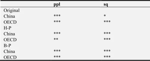
But authors can still draw some conclusion about the significance of the explaining variables. For convenience, authors use the p-value test method. To make the result more obvious, authors use the Null, *, **, and *** to indicate the p level of (0.9,1], (0.8,0.9], (0.7,0.8], (0,0.7]. See the result in Table 1 as following.
Table 1. Significance of the variables.
ppl sq
Original
China *** *
OECD *** ***
H-P
China *** ***
OECD ** ***
B-P
China *** ***
OECD *** ***
4.3. Comparison Between China and Other Developing Country
The research results of these countries listed above seem quite so reasonable, but these result and analyses are based on the OECD countries and China. These countries are all modern countries (Authors define the modern countries as those own modern government and the governments can execute macro-economy management.). But how about other countries?
For a long time, China and India have been regarded as two similar countries. These two countries are similar to each other
both in location, population, culture and in developing stage. So authors take the data of India and China for contrast (without any filter).
Table 2. Significance of the variables of China and India.
country country special and
international impact factors population
financial market size
China ** *** ***
India ***
As for the standard deviation, the standard deviation of India GDP (from after taking the logarithm but without nay filter process) equals 0.51184376, and that of China is 1.228820526. Authors can draw to a conclusion with the confidence level of more than 0.975 that these variances are different from each other.
After analysing this comparison, authors took the result as a real odd, because for India, the impacts caused by population and financial markets (or to be specific, the impacts of consumption and investment) are both not quite so significant, so there must be other factors contributing to its business cycle volatility (As authors listed in the chart above, some other explaining variables like the country special and international impact factors.).
5. Conclusion and Analysis
5.1. Model Analyses
The regression coefficient of financial market volume of China is much larger than that of OECD countries, but after the data of China were H-P filtered, the regression coefficient suddenly became negative. This result tells us that there are many high frequency fluctuations in the business cycle of China caused by the speculation behaviors in the investment department (to be more precise in the stock market).
But if researchers do not limit research area on the thesis of Davide Furceri and Georgios Karras, and check the model itself, authors have found that themselves could not accept the linear model itself. After F-test, the linear model cannot be accepted at the confidence level of 0.9.
5.2. Coefficient Analyses
When authors examine the original result, it is obvious that for OECD countries the regression coefficient of population is negative while that of financial market is positive. The result of the first regression coefficient consistent with the research result of Furceri, while the latter one indicates that even for the OECD countries whose financial markets are normative, the investment departments can also increase the business cycle volatility. But for China, both these regression coefficients are positive. And the constant term of China is much larger than that of OECD countries.
over the past 20 years.
Maybe the influence of other departments like the real estate and net export should not be neglected. Also some previous scholars ever focused on the impact of insurance industry, they have found that in the countries (like the OECD countries) where the insurance industries can provide perfect or approximately perfect insurance, the consumption shocks in their consumption department can be significantly weakened, and as a result, their business cycle volatilities can be greatly decreased in this way. [14]
According to the database of National Bureau of China, during that period of time housing sell and export account for more than 40% of the total GDP of China and they maintain the similar proportion in the several years before and after that period of time. Also in the history, economists have ever confirmed that the housing industry can be a source of power driving the business cycle[15] so the fluctuations of them must have contribute to the business cycle volatility of China.
5.3. Fluctuation Analyses
After two methods of filter, the significant levels of financial market on China both increased. These results may indicate that the Chinese financial market attributes to both the high frequency and the high amplitude fluctuations of the volatility of Chinese business cycle. Indeed, it is widely possible that this influence is an industrial structure impact.
5.4. Variable Analyses
The constant item of the regression formula of China is always much larger than that of OECD countries. So it is widely possible that in China there some other investment aspects, which contribute to the business cycle volatility. (Authors will give some possible explanations in the following parts.)
Another question, as authors have said, for the sample countries authors have chosen the relation between the GDP and the listed company total value is strong linear relation, so authors can use the latter in place of GDP. But for the developing countries, this relation may not work (and some countries even do not have stock exchange market at all!) Is the economic scale of a certain country not so essential? Of course not, and authors will give a proceeded explanation later.
Another interesting phenomenon is that after the high frequency fluctuations were filtered out the significance level of variable population decreased. It seems that the population (or to be specific, the consumption department) contributes the high frequency fluctuations in the business cycle. Indeed the situation is not quite so direct: For the OECD countries, the governments can execute powerful macro-economy management and of the several fiscal instruments that can be used. The government consumption is among the most powerful instruments. Increase in government consumption amplifies the decline in private consumption generated by the recessionary shocks. In this respect, the use of the consumption tax squeeze out some potential contribution of
private consumption [16]. And in this way, can we understand why the significance of population decreased here.
6. Further Study
6.1. The Analyses of the Explaining Variables
Up to now, the relevant researchers (including Furceri, Karras and authors) have judged the influence of country size (measured by population) and capital market scale on the business cycle volatility. But the business cycle is a widely complicated problem. For example, if researchers would like to study the business cycle thoroughly, the real estate should be taken into account, especially for China. At least from authors’ perspective, when we take the housing industry into account to explain the long period business cycle problem and the time span should be longer and approximate to that of Konddratieff Cycle.
Furthermore, as E. F. Fama has argued, the efficiency of financial markets can be ranked in at least three different levels, and it is impossible that all the stock markets of OECD countries are at the same level [3]. So, to make the theory more considerate, maybe researchers should examine the efficiency degree of these countries before regression operation. Furthermore, researchers have made an over simplified assumption that the stock market volume at a certain time will not influence the volume in the next period of time. (Or rather say that researchers including authors have used the non-aftereffect regression model.) According to the theory of EMH by E. F. Fama [3], this assumption can only work in what is called Strong Form of Efficient Markets, but up to now, there has not been even one such financial market exist in the world. Even the financial market of the United States is merely approximate to Strong Form of Efficient Markets.
So to make this regression analyses more preciseness, later researchers must use the Markov process [17] and use the transaction data (the market value of listed companies does not have the direct relation with the calculation of gross domestic product) only in this way can the latter researchers determine the exact influences of investment department on the business cycle of macro-economy.
6.2. The Analyses of Those Control Variables
Up to now, both Furceri and the authors follow the selection of variable set of Rose [11]. And maybe it is due to this simplifying assumption that authors obtained a random effect regression.
But in the real macro-economy system, there are far more factors that can either drive the business cycles or influence the volatility of them. (The regression result of India as authors have talked above is a good example.)
macroeconomy management including the fiscal polices) can attribute to reduce the volatility of the business cycle. And these factors may be more complicated and less significant in the developed countries like the OECD members.
Even within those developed countries the governments’ behaviors should not be neglected and it is quite a complicated factor. Despite though the direct way of squeezing out the consumption authors mentioned above, moreover the governments can also affect the inflation rate [18] and thus indirectly influence the business cycle.
6.3. Analyses of the Model
Future researchers must also address a peculiar contradiction between theory and empirical evidences regarding scale effects. While numerous theoretical growth models predict scale effects on steady state growth and the levels of net domestic income, these effects have not been easy to detect empirically, so it is listed in the list of control variables by the researchers from Rose to the authors.
At the same time, while the empirical evidence has pointed out the significant scale effects of GDP on cyclical fluctuations, theoretical business-cycle models normally ignore country economic size itself as an explaining variable. The results of this paper suggest that this is an omission worth addressing. Directly, there is a famous gravity model of trade, in which Tinbergen indicated (1962) that the total GDP of a country has significant influence (in his model to be exact, determines) the scale of international trade. As a result, it will influence the volatility of itself in another (a way differ from that through stock market) approach.
So in a word, to make this model more convictive, the latter researchers should contain other factors (at least the economic aggregate) in their explaining variables.
References
[1] Nektarios Aslanidis; Charlotte Christiansen; Neophytos Lambertides; Christos S. Savva. Idiosyncratic Volatility Puzzle: Influence of Macro-Finance Factors [J]. Aarhus University in its series CREATES Research Papers with number 2014-45, 2014.
[2] Emiel F. S. van Bezooijen; Jacob A. Bikker. Discussion Paper Financial Structure and Macroeconomic Volatility a Panel Data Analysis [J]. Discussion Paper Series nr: 17-13, 2017. [3] Burton G. Malkiel; Eugene. F. Fama. Efficient Capital Markets:
A Review of Theory and Empirical Work [J]. The Journal of Finance. Pages 383–417 May 1970.
[4] Furceri. Country size and business cycle volatility [J]. Journal of the Japanese and international economies 21 (2007) 424– 434, 2007.
[5] Jan Tinbergen. Statistical Testing of Business Cycle Theories: Part II: Business Cycles in the United States of America, 1919-1932 [M]. Agaton Press, 1968.
[6] Nam T. Vu. Stock market volatility and international business cycle dynamics: Evidence from OECD economies [J]. Journal of International Money and Finance 50 (2015) 1e15, 2015. [7] Yung-Shun Tsai; Chun-Ping Chang; Shyh-Weir Tzang; The
Impact of Stock Prices, Risks, and Business Cycle on Overconfidence [J]. 2016 10th International Conference on Innovative Mobile and Internet Services in Ubiquitous Computing, 2016.
[8] Mark J. Holmes, Nabil Maghrebi. Financial market impact on the real economy: An assessment of asymmetries and volatility linkages between the stock market and unemployment rate [J]. The Journal of Economic Asymmetries 13(2016)1–7, 2016. [9] Theofanis Papageorgiou; Panayotis G. Michaelides; Efthymios
G. Tsionas. Business cycle determinants and fiscal policy: AP anel ARDL Approach for EMU. [J] The Journal of Economic Asymmetries 13(2016)57–68, 2016.
[10] Hodrick, Robert; Prescott, Edward C "Postwar U.S. Business Cycles: An Empirical Investigation". Journal of Money, Credit, and Banking [J]. 29 (1): 1–16. JSTOR 2953682, 1997. [11] Rose, A. K.. Size really doesn’t matter: In search of a national
scale effect. J. Japanese Int. Economies 4, 482–507. [J], 2006. [12] Hausman, J. A. "Specification Tests in Econometrics" [J].
Econometrica. 46 (6): 1251–1271, 1978.
[13] Davide Furceri; Georgios Karras. Business cycle volatility and country zize; evidence for a sample of OECD countries [J], 2008.
[14] Jonathan McCarthy. Imperfect insurance and differing propensities to consume across households [J]. Journal of Monetary Economics, 1995.
[15] Simon Kuznets. Secular Movements in Production and Prices [M], 1930.
[16] S. Gomes; P. Jacquinot; R. Mestre; J. Sousa. Global policy at the zero lower bound in a large scale DSGE model. [J] Journal of International Money and Finance 134e153, 2015.
[17] Takamitsu Kurita. Markov-switching variance models and structural changes underlying Japanese bond yields: An inquiry into non-linear dynamics [J]. The Journal of Economic Asymmetries 13 (2016)74–80, 2016.