http://www.sciencepublishinggroup.com/j/acm doi: 10.11648/j.acm.s.2018070101.11
ISSN: 2328-5605 (Print); ISSN: 2328-5613 (Online)
Convergence Analysis of Piecewise Polynomial Collocation
Methods for System of Weakly Singular Volterra Integral
Equations of The First Kind
Gholamreza Karamali
1, Babak Shiri
1, 2, *, Mahnaz Kashfi
21
Shahid Sattari Aeronautical University of Science and Technology, South Mehrabad, Tehran, Iran
2Department of Applied Mathematics, University of Tabriz, Bahman Boulevard, Tabriz, Iran
Email address:
[email protected] (G. Karamali), [email protected] (B. Shiri), [email protected] (M. Kashfi)
*Corresponding author
To cite this article:
Gholamreza Karamali, Babak Shiri, Mahnaz Kashfi. Convergence Analysis of Piecewise Polynomial Collocation Methods for System of Weakly Singular Volterra Integral Equations of The First Kind. Applied and Computational Mathematics. Special Issue: Singular Integral Equations and Fractional Differential Equations. Vol. 7, No. 1-1, 2018, pp. 1-11. doi: 10.11648/j.acm.s.2018070101.11
Received: March 21, 2017; Accepted: March 22, 2017; Published: April 11, 2017
Abstract:
We study regularity of solutions of weakly singular Volterra integral equations of the first kind. We then study thenumerical analysis of discontinuous piecewise polynomial collocation methods for solving such systems. The main purpose of this paper is the derivation of global convergent and super-convergent properties of introduced methods on the graded meshes. We apply relevant methods to a system of fractional differential equations and analyze them. The numerical experiments confirm the theoretical results.
Keywords:
Discontinuous Piecewise Polynomial Spaces, Collocation Methods, Graded Meshes,Weakly Singular Volterra Integral Equations
1. Introduction
In this paper, we consider a system of weakly singular Volterra integral equations of first kind (SWSVIEFK) of the form
0
( , ) ( )
( ), : [0, ],
( )
tk t s y s
ds f t t T
t−sα = ∈ =
∫
I (1)where, 0< <α 1, T∈R,ν∈N, f :I→Rν. The domain of the matrix function k t s( , ) :D→Rν ν× , is
2
{( , ) | ( , )t s t s , 0 s t T}.
= ∈ ≤ ≤ ≤
D I
Also, we suppose that k t t( , ) is a nonsingular matrix for all .
t∈I The y:R→Rν is the unknown vector function. The
system (1) is an Abel's integral equation if k t s( , )=1.
The numerical solution of weakly singular Volterra integral equations of first kind has extensively been studied (see for example [2, 3, 4, 5, 6, 8, 9, 10, 11, 13, 14, 15, 16], but it does
not mean that this subject has completely been studied. There are some unsolved problems which are important and need more challenge. One of them is convergence analysis of collocation methods on the piecewise polynomial spaces for solving system (1), [3]. The aim of this paper is to provide a complete convergence analysis of these methods for this system.
The piecewise polynomial collocation methods (PPCM) are easily programmable and they have rapid convergent order for many equations including integral or differential operator. They have extensively been examined by many authors. We refer here to [1, 3, 7, 12] and literature given therein. Therefore, it is important to analyze PPCMs for the system (1).
Suppose ν∈N. Let q:R֏R and f:Ω֏Rν ν× be
scaler and matrix functions, respectively, where Ω is a set. In this paper, by qf we mean
, {1, , } ,
maxi j sup | i j( ) | .
t
f ∈ ν f t
∈Ω
= ⋯
‖ ‖
The paper is organized as follow:
In section 2, we review existence, uniqueness and smoothness of the solutions of system (1). In section 3, we recall application of the collocation method on the continuous piecewise polynomial spaces. In section 4, we generalize Granwall’s inequalities for matrix function equations. In section 5, we give the global convergence of the collocation method on the continuous piecewise polynomial spaces. In section 6, we investigate the stability function introduced in the previous section. Finally, in section 7, we present numerical experiments which support theoretical results.
2. Regularity Properties
The arguments of this section can be obtained by arguments similar to [3] (section 2.1.1). Here, we should concern that the systems we investigated are of dimension greater than 1 while the system in [3] is of dimension greater 1. Therefore, instead of dividing by a function we should multiply by an inverse of corresponding matrix function.
Suppose Gα∈
(
C I( ))
ν and1 1
0
( )
( ) sin ( , )d z ( )( ) .
G z k z z f t z t dt
dz
α α
πα π
− −
=
∫
− (2)Define resolvent kernel associated with the given kernel ( , )
Kα z s as
1
( , ) : lim ( , )
n
n n
i
R z s H z s
→∞ =
=
∑
where
1 1
( , ) z ( , ) ( , ) , 2,
i s i
H z s =
∫
H z v H− v s ds i≥and 1
1 1
1 0
( ) ( ( ), )
( , (z,s)=
) .
(1 ) H
sin k s z s s
k z z d
z α α
πα ν ν
π ν ν
−
−
∂ + −
−
∂
∫
−Then, we obtain corresponding Volterra’s fundamental results that
0
( ) ( ) z ( , ) ( ) .
y z =Gα z +
∫
R z s G s dsα (3) is a unique solution of system (1). Now, we can argument about the regularity of solutions. Supposing(
m( ))
k∈ C D ν ν× and
(
m( ))
,k
t
ν ν×
∂ ∈
∂ C D we obtain 1( , )
(
( ))
.m z s
H ∈ C D ν ν× It is
straightforward then to show that ( , )
(
m( ))
.R z s ∈ C D ν ν×
Therefore, the regularity of y depends on the regularity of Gα.
Theorem 2.1Let
(
m( ))
,k∈ C D ν ν× k
(
m( ))
,t
ν ν×
∂ ∈
∂ C D m∈N,
( ) ( )
f t =t g tβ where g∈
(
Cd([0, ])T)
ν, 1≤ ≤ +d m 1, d∈N,and
β
≥ −1α
. Then, the system (1) has a unique solution and there exists(
1)
([0, ])
d
q∈ C − T ν such that 1
( ) ( ).
y z =zα β+ −q z Proof. Integrating by substitution t=vz, we have
1
0 0 ( )( ) ( )
z
t g t zβ −tα−dt=zα β+ q z
∫
Where
1 1
0( ) : 0 ( )(1 ) ,
q z =
∫
v g zvβ −vα −dvand hence we obtain
(
)
1 0
1 (1)
0 0
( )( )
( ) ( ) ( ) .
z d
t g t z t dt
dz
z zq z q z
β α
α β α β
− + −
−
= + +
∫
Since g∈
(
Cd([0, ])T)
ν, we conclude that(
)
0 ([0, ]) ,
d
q ∈ C T ν
and consequently
(
)
(1) 1
0 ( ) ( ) 0( ) ([0, ]) .
d
zq z + α β+ q z ∈ C − T ν
Thus, using equation (2), there exists
(
1)
1 ([0, ])
d
q ∈ C − T ν
such that 1 1
( ) ( ).
Gα z =zα β+ −q z Taking into account that
(
)
2
0 1
1 0
1
1 1
1 0
1
( ) : ( , ) ( )
( , )
( )
( , ) ( ) ([0, ]) ,
z
z
d
q z R z s G s ds
z R z s
s q s ds
z
R z vz v q vz dv T
α α β
α β α β
ν α β
+
+ − +
+ − −
=
=
= ∈
∫
∫
∫
C(4)
and using the equation (4), we have
1
1 2
( ) ( ( ) ( )),
y z =zα β+ − q z +zq z
which completes the proof.
3. Collocation Method on the Continuous
Piecewise Polynomial Spaces
For given N∈N, Let
{ ( ) : 0r },
h n
n
I t T n N
N
be a graded mesh, with grading exponent r≥1. Assume that
1
( , ],
n t tn n
σ = + σn=[ ,t tn n+1], hn =tn+1−tn and max{ j: 0, , 1}.
h= h j= ⋯ N− Then, it is straightforward to see
that the sequence { } 0
N n n
h = is strictly increasing and
1
1 , 0, , 1.
j N
h ≤ =h h − <rTN− j= ⋯ N−
(5)
We use collocation method to solve system (1) directly (without transforming to the second kind integral equation), on the discontinuous piecewise polynomial spaces
( 1)
1( ) : { : |n 1( 0,1,..., 1)}, .
m Ih v v σ πm n N m
−
− = ∈ − = − ∈
S N
For discontinuous piecewise polynomial spaces, let
1
0< <c ⋯<cm ≤1, m∈N be the collocation parameters.
Therefore, the approximate solution
(
( 1))
1( ) ,h m h
u ∈ S−− I ν has the
form
, 1
( ) ( ) , (0,1], 1, , 1,
m
l l l j l j
j
u t vh L v U v l N
=
+ =
∑
∈ = ⋯ −in the interval σl ( | , l
l h
u =u σ for l=1,⋯,N−1). Here, L (v)j for j=1,⋯, ,m are Lagrange fundamental polynomials with
respect to distinct collocation parameters and U :=u (t )l,j h l,j are approximation solutions at the collocation points
, :
l j l j l
t = +t c h for l=1,⋯,N−1 and j=1,⋯, .m We are seeking for a collocation solution uh such that satisfies the collocation conditions
, ,
, 0
,
( , ) ( )
( ),
( )
n i
t
n i h
n i n i
k t s u s
ds f t
t −s α = ±
∫
(6)for n=0,⋯,N and i=1,⋯, .m Therefore, it is
straightforward to show that the solution of the system (6) can be obtained by solving recursively the systems
,
, 0 , ,
1 ,
( , ) ( )
( ) ( )
( )
i
m
c n i n n j
n i n n j n i
j n i n n
k t t vh L v
F t h dvU f t
t t vh α
=
+
+ =
− −
∑ ∫
(7)for i=1,⋯, ,m and n=0,⋯,N−1, where
1
1 ,
, ,
0 0 1 ,
( , ) ( )
( )
( )
n m
n i l l j
n i l l j
l j n i l l
k t t vh L v
F t h dvU
t t vh α
− = =
+ =
− −
∑ ∑ ∫
is the lag term. In the system (7), the integrals can be approximated by the quadrature approximations
,
, , , 0
,
( , ) ( ) 1
( ) ( , )
( )
i
c
n i n n j
i j n i n j
n i n n n
k t t vh L v
dv a k t t
t t vh α hα α
+ − −
∫
≃and
1 ,
, , 0
,
( , ) ( ) 1
( , , ) ( , ),
( )
n i l l j
ij n i l j
n i l l l
k t t vh L v
dv b n l k t t
t t vh α hα α
+ − −
∫
≃For 0≤ ≤ −l n 1, where
, 0
( ) ( )
( )
i
c j
i j
i
L v
a dv
c vα
α
=−
∫
and
1 0
,
( )
( , , ) , 0 1,
( )
j ij
n i l
l
L v
b n l dv l n
t t v h
α
α = − ≤ ≤ −
−
∫
for i j, ∈{1,⋯, }.m Therefore, the fully discretised version can be obtained by solving the systems
1
, , , , , ,
1
ˆ( ) m ( ) ( , )ˆ ( ),
n i n i j n i n j n j n i
j
F t h−α a α k t t U f t =
+
∑
= (8)recursively, for i=1,⋯,m and n=0,⋯,N−1, where
1 1
, , , ,
0 1
ˆ( ) n m ( , , ) ( , )ˆ ,
n i l ij n i l j l j
l j
F t h α b n lα k t t U −
−
= =
=
∑
∑
for i=1,⋯, ,m and
,
ˆ
l j
U are the collocation solution at tl j, for
0, , 1
l= ⋯ N− and j=1,⋯, .m Now, the dense output approximate solution can be approximated by
, 1
ˆ
ˆ ( ) ( ) , (0,1], 1, , 1.
m
l l l j l j
j
u t vh L v U v l N
=
+ =
∑
∈ = ⋯ −We note that this discretised version is slightly different from discretised version introduced in [3]. However, it reduce the computation complexity by a factor of 1,
m and as we will
see it does not reduce the order of the collocation method. Setting (A3) :ij =aij( ),α ˆ : [ɵ ,1, , ˆ , ] ,
T n
n n m
U = U ⋯U
,1 ˆ ,1 , ˆ ,
[ (f tn ) F t(n ), , (f tn m) F t(n m)] ,T
= − ⋯ −
F and taking into
account that
, ,
(
n i,
n j)
( , )
n n( ),
k t
t
=
k t t
+
O
h
we can write (8) in the matrix form
ɵ
1
3 ( ( , ) ( )) n .
n n n n n
h−αA ⊗ k t t +O h U =F
Now, since A3 is invertible by Theorem 6.1, and k t t( , )n n
is invertible by hypotheses of the introduction, the matrix
3 ( ( , )n n ( n))
A ⊗ k t t +O h is invertible and there exists a unique
4. Granwall’s Inequalities
First, we recall the Granwall’s inequalities [3]. Note that, we write
( m) whenever ( m).
v=O h ‖ ‖v =O h
Lemma 4.1. (Gronwall's inequality) Assume that{ }kj ,
(j≥0) is a given non-negative sequence and the sequence { }εn satisfies
0 ≤ρ0
ε and
1 1 0
0 0
n n
n j j j
j j
q k
ρ − −
= =
≤ +
∑
+∑
ε ε
with ρ0≥0 and qj≥0for(j≥0). Then
1 1
0
0 0
exp .
n n
n j j
j j
q k
ρ − −
= =
≤ +
∑
∑
ε
In this paper, we need a generalization of Gronwall’s inequality for the matrix functions. Thus, we consider
1
1 0
0
n
n n j j
j
R K ρ
− −
=
= +
∑
+ε ε ε
(9)
where R, ρ0, Kj and εj for j=0,1,⋯, are matrix functions.
We suppose that R is a diagonalizable matrix i.e.,
1
,
R=P DP− where D=diag( ,λ1⋯,λr) is a diagonal matrix and P is a nonsingular matrix. Also, we suppose that
[ 1,1).
i
λ ∈ − Then, It is straightforward to show that there exists a positive constant Csuch that
(
)
10 0
0
exp .
n
n j
j
C ρ C K
− =
≤ +
∑
ε ε
‖ ‖ ‖ ‖ ‖ ‖ ‖ ‖
5. Global Convergence
5.1. Discontinuous Collocation Method
Lemma 5.1. For r≥1, we have
1 ( 1) 1
1 ( ) 1 ( ).
( 1) ( )
r r
n
n
r r
n
h n n
O h
h n n n
− = − − = − = +
+ − O
Hence
1
1 1
1 1 ( ),
n
n n
h
O h h
α
α α
−
− −
− = −
and similarly
1
(1 n ) ( ).
n n
h
O h h−
− =
O
Proof. One can easily observe the results by expanding the polynomials ( 1)r
n+ and ( 1)r
n− for case r∈N. The other
cases can be obtained by applying the Hopital’s rule. Theorem 5.2. Let k∈
(
Cm( )D)
ν ν× , k(
m( ))
,t
ν ν×
∂ ∈
∂ C D
,
m∈N f t( )=t g tβ ( ) where g∈
(
Cd([0, ])T)
ν, 1≤ ≤ +d m 1, ,d∈N and β ≥ −1 α. Then the approximate solution uhof
the discontinuous collocation method for system (1) with collocation parameters 0< <c1 c2<⋯<cm ≤1 and the
grading exponent r≥1 converges to the solution if the eigenvalues of the stability matrix ℜ be in the interval [ 1,1).− Furthermore, the collocation error satisfies
( 1)
1
1
, 1 ,
1 ( ) ( )
1
, ,
1
r
h
d
d
N r
y t u t c
d
N r
α β
α β
α β − + −
− +
− ≤ ≤
+ −
− ≤
− ≥
+ −
‖ ‖
for a constant c>0 and sufficiently large N.
Proof. Suppose that the assumptions of Theorem \ref{th1} hold. Let e th( )=y t( )−u th( ). An application of Theorem 2.1 implies that
(
1)
([ , ])
d
y∈ C − εT ν for all ε>0. Therefore, by Peano’s theorem ([3], Section 1.8)
, 1
( ) ( ) l ( )
m
h l l j l j l l
j
e t vh L v E h R vλ
=
+ =
∑
+ (10)where El j, =e th(l+c hj l) for j=1,⋯, ,m l=0,⋯,N, the
remainder R vl( ) is a bounded function and
1, 0,
1, Otherwise.
l
l
d
β α
λ = + − =
−
(11)
By subtracting equation (1) (at t=tn i, ) from equation (6)
we obtain
, , 0
,
( , ) ( ) 0,
( )
n i
t n i h
n i
k t s e s
ds
t −sα =
∫
(12)for n=1⋯,N−1, i=1,⋯, ,m and hence,
1
,
1 , 0 ,
, ,
( , ) ( )
( )
( , ) ( ) 0.
( )
l l
n i n
n
t n i h
t
l n i
t n i h
t n i
k t s e s
ds
t s
k t s e s
ds
t s
α
α
+
−
= −
+ =
−
∑∫
∫
(13)
Letting n=0,substituting s=vh0, and using (10) we have
0
0 0
0, 0
1
0 0
( , )
( )
( )
( ) , i
i
m c
i
j j
j i
c
l k c h vh
L v dvE
c v
h R v dv
α
λ =
= −
−
∑ ∫
∫
(14)
for i=1,⋯, .m By Taylor's theorem for multivariable matrix
be written in the matrix form
0
3 0 0 0
(
A
⊗
k
(0, 0)
+
O
(
h
))
E
=
O
(
h
λ)
where 0 [ 0,1, , 0, ]
T m E E = … E and 3 0 ( )
( ) , , {1, , }.
( ) i c j ij i L v
A dv i j m
c v α
= ∈
−
∫
⋯ (15)Since, A3 and k(0, 0) are invertible matrices, we can conclude that 0
0,j (h0 ),
λ
=
E O for sufficiently small h. We can
now proceed to obtain an estimate for | , n
n h
e =e σ n∈N.
Substituting s= +tl vhl, l=0,⋯, ,n into corresponding
integrals in (13) and using (10) we obtain
2
1 , 1,
, 0
0 1 , 1,
1 , 1 1
1 0 1,
1 , 1 1 , 0 1 , ( , ) ( , ) ( ) ( ) ( ) ( , ) ( ) ( ) ( , ) ( ) ( ) i n m
n i l l n m l l
l j l j
l j n i l l n m l l
m
n i n n j
n n j
j n i n n
c n i n n j
n
j n i n n
k t t sh k t t sh
h L s dsE
t t sh t t sh
k t t sh L s
h dsE
t t sh
k t t sh L s
h
t t sh
α α α α − − = = − − − − − = − − = + + − − − − − + + − − + + − −
∑ ∑ ∫
∑ ∫
∫
,1, 1 1
1 0 1,
1 1, 1 1
( , ) ( ) ( ) ˆ m m n j m c
n m n n j
n n j
j n m n n
n
dsE
k t t sh L s
h dsE
t t sh
R α − − − − − = − − − + − − − =
∑
∑ ∫
(16)Rewriting (16) with replacedn by n−1 and j=m and subtracting it from (16), we obtain
2
1 , 1,
, 0
0 1 , 1,
( , ) ( , )
( )
( ) ( )
n m
n i l l n m l l
l j l j
l j n i l l n m l l
k t t sh k t t sh
h L s dsE
t t sh α t t sh α
− − = = − + + − − − − −
∑ ∑ ∫
1 , 1 1
1 0 1,
1 , 1 1 ,
, 0
1 ,
1, 1 1
1 0 1,
1 1, 1 1
( , ) ( ) ( ) ( , ) ( ) ( ) ( , ) ( ) ( ) ˆ i m m
n i n n j
n n j
j n i n n
m
c n i n n j
n n j
j n i n n
m c
n m n n j
n n j
j n m n n
n
k t t sh L s
h dsE
t t sh k t t sh L s
h dsE
t t sh
k t t sh L s
h dsE
t t sh
R α α α − − − − = − − = − − − − − = − − − + + − − + + − − + − − − =
∑∫
∑ ∫
∑ ∫
(17) where 2 1 , 1, 00 , 1,
ˆ
(
,
)
(
,
)
( )
(
)
(
)
l n nn i l l n m l l
l l l
l n i l l n m l l
R
k t
t
sh
k t
t
sh
h
h R s ds
t
t
sh
t
t
sh
λ α α − − = −
−
=
+
+
−
− −
− −
∑ ∫
1 1 01 , 1 1 1 1 1 0
1 1 ,
0
1, 1 1 1 1 1 0 1 1 0 1 ( , ) ( )
( 1 )
( , ) ( ) ( ) ( , ) ( ) ( ) ( ) , n n i n m
n i n n n n
n
n
n i
n
c n i n n n n
n
n i
c n m n n n n
n n m d n n n
k t t sh h R s
h ds
h
h c s
h
k t t sh h R s
h ds
h c s
k t t sh h R s
h ds
h c s
h h h h λ α α λ α α λ α α λ α − − − − − − − − − − − − − − − − − − + + + − + + − + − − = +
∫
∫
∫
O (18)by Lemma 5.1 and following Remark. Remark 5.3. We note that,
(
1, ,)
( , )
( , ) ([ , ] [0,1]) ,
( )
m
l l
n m n m
l l
k x t sh
x s C t t
x t sh
ν ν α × − + ∈ × − −
֏ for
0, , 2.
l= ⋯ n− Therefore, if we apply mean value theorem for
each components of the above matrix function, then we have
, 1,
, 1,
( , ) ( , )
( ) ( )
( ).
n i l l n m l l
n i l l n m l l
n i l l
k t t sh k t t sh
t t sh t t sh
h k t sh
α α − − + + − − − − − = + (19)
where there exist tn−1,m ≤pqθi l, ≤tn m, such that
, 1
,
( ( ))
( , )
( (1 ) )
( )
i l l pq
pq
pq i l l l
n
i m
n pq i l l l
k t sh
k
t sh
h t
c c
h t sh α
θ θ − + ∂ + ∂ = + − − −
for p q, ∈{1,⋯, },ν i=1,⋯,mand l=0,⋯,n−2. By our assumptions k
t ∂
∂ is bounded and there exists M >0
such that 1
( (1 ) n ) .
i m
n
h k
c c M
h t
− ∂
+ − <
∂
‖ ‖ Therefore,
1 0 1 0 , 1 0 1, |( ( )) ( ) | | ( ) | ( ) | ( ) | ( ) 2
( 1 ) ,
(1 )
i l l pq j
j
pq i l l l
j
n m l l
l
k t sh L s ds
M L s ds
t sh
M L s ds
t t sh
M n l h α α α α α θ α − − + ≤ − − ≤ − − ≤ − − −
∫
∫
∫
(20)for l=0,⋯,n−2. The last inequality is obtained by Lemma (6.2.10) [3]. Also, setting
2 ( ) , (1 ) M α γ α α = −
1
0( (k ti l shl))L s dsj( ) ( )hl (n 1 l) .
α α
γ α − −
+ ≤ − −
∫
‖ ‖ (21)
Furthermore, to obtain equation (18), we use the fact that the sum
2 1 0
( 1 )
n
l l
h α n l α
−
− −
=
− −
∑
is bounded.Substituting (19) into (17), and using Taylor's series for other terms and components we obtain
2
1
, 0
0 1
1 1 2 1
1 0 1,
1 1 1 3 , 0 1 ( ) ( ) ( ( , ) ( ) ( ) ) ( )
( 1 )
( ( , ) ( ) ) ( )
( )
i
n m
l n i l l j l j
l j
m
n n n n j
n n j
j n
n i
n
m
c n n n j
n n j
j n i
h h k t sh L s dsE
k t t c s h c s h L s
h dsE
h
h c s
h
k t t c s h L s
h dsE
h c s
α α α α − = = − − − = − − = + + + + + − + + −
∑
∑ ∫
∑ ∫
∑ ∫
4 1 1 1, 0 1 1 ( ( , ) ( ) ) ( ) ( ) ˆ m mc n n n j
n n j
j n m
n
k t t c s h L s
h dsE
h c s
R α α − − − = − + − − =
∑ ∫
(22)where c si( ) for i=1,⋯, 4 are bounded matrix functions. Multiplying (21) by 1
( ,n n)
k t t
−
=
k and dividing by hn, we obtain 2 1 , 0 0 1 1 1
1 1 2 1
1 1, 0 1 1 1 ( ) ( )
(1 ( ) ( ) ) ( )
( 1 )
n m
l i l l j l j
l j
m
n n j
n n j j n n n i n
h k t sh L s dsE
c s h c s h L s
h dsE h h h c s h α α − = = − − − − − = − − + + + + + −
∑ ∑ ∫
∑ ∫
k k1 3 , 0 1 1 4 1 1 1, 0 1 1
(1 ( ) ) ( )
1
( )
(1 ( ) ) ( )
( ) ˆ . i m m c n j n j j n i m c n j n n j j
n n m
n
n
c s h L s dsE
h c s
c s h L s
h
dsE
h h c s
R h α α α α − = − − − − = − + + − + − − =
∑∫
∑ ∫
k k (23) Denoting, 1 ( ) , 0 1 11 , 0
2 , 0
3 , 0
1 1 1 2 1 (1) 1 , 0 1
( ) : ( ) ( ) , 0, , 2,
( )
( ) : ,
( 1 )
( ) ( ) : , ( ) ( ) ( ) : , ( ) ( ( ) ( )) ( ) ( ) :
( 1 )
m
i
m l
n i j i l l j j j i j i c j i j m c j i j i n j n
n i j
n i
n
k t sh L s ds l n
L s ds c s L s ds c s L s ds c s h
c s c s L s h ds h c s h α α α α = − − − − = + = − = + − = − = − + = + −
∑ ∫
∫
∫
∫
∫
⋯ B A A A k k K 1 3 ( 2) , 0 1 4 0 ( ) ( ) ( ) : , ( ) ( ) ( ) , ( ) i m c jn i j
i
c j
m
c s L s ds
c s
c s L s ds c s α α − − = − − −
∫
∫
k K kand we can rewrite system (22) in the matrix form
(
)
2 ( ) 0 (1) 11 1 1
1 ( 2) 3 ( ) ˆ 1 ( ) , n l
l n l
l
n
n n n n
n n
n
n n n
n n h h h h h h R h h h ν α ν α − = − − − − + + − + ⊗ + + ⊗ =
∑
2 BA A K I
A K I
E
O E
E
(24)
where Iν is identity matrix of dimension
ν
. Multiplying equation (23) by(
( 2 ))
1 ( 2) 13 3
( hn n ) ν ( hn n ) ν
− −
+ ⊗ = + ⊗
A K I A K I
(which exists for sufficiently small h, by Theorem 6.1), we obtain 0 1 1 1 1 2
( ) 1 0 0
( ( ))
( ).
n
n n n
n
n
l d
l n n l n
l h
h h
h h h h
α α λ α − − − − − − =
= ℜ +
+
∑
C + +E O E
E O
(25)
where ( ) ( 2 ) 1 ( ) 3
( )
l l
n hn n ν n
−
= − + ⊗
C A K I B and
(
)
1
3 2 1
( )− ν.
ℜ = A A −A ⊗I
Using Lemma 5.1 we can conclude that
0
1 1 2
( ) 1 0 0
( ( ))
( )
n n n
n
l d
n l n l n
l h
h h h h
α λ α − − − − =
= ℜ +
+
∑
C + +E O E
E O
and by (5) we have
0
1
1 1
2
( ) 1 0 0
( )
( ).
n n n
n
l d
n l n l
l
h
h h h h
α λ α − − − − − =
= ℜ +
+
∑
C + +E E O E
E O (26)
If eigenvalues of the stability matrix ℜ be in the interval [ 1,1),− we can invoke generalized Granwall's inequality to conclude that
(
0 1)
0 0 2
( ) 1 0
( )
exp ( )
d n
n
l
n l n
l
C h h
C h h h
λ α α − − − = = + + × +
∑
C E E O
O
‖ ‖ ‖ ‖
‖ ‖ (27)
where C>0 is a constant.
0
M > such that
( 2 ) 1 3
( 2) 1 3
( )
( )
( )
( )
n n
n n
h
M
h
M
ν
ν γ α
γ α −
−
+ ⊗
≤ + ⊗
≤
A K I
A K I
‖ ‖
‖ ‖
by (21), ( ) ,
( l) ( ) ( 1 )
n i j hl n l
α γ α −
≤ − −
B
‖ ‖ and therefore
( ) ,
( l) ( 1 ) .
n i j M n l hl
α α − −
≤ − −
C
‖ ‖ (28) Consequently, the equation (28) yields
2 2
( )
0 0
2 1 0
1 0
1
1
( 1 )
( 1 )
( 1 )
( 1) 1 ( 1)
(1 ) . (1 )
n n
l
n l n
l l
n l
l l
n
h h hM n l
hM n s ds
hM n s ds
n hM
N rTM
N
rTM
α α
α
α α
α α
α
α
− −
−
= =
− +
− =
− −
− +
− +
≤ − −
≤ − −
= − −
− =
− − ≤
−
≤ −
∑
∑
∑ ∫
∫
C‖ ‖
(29)
Taking into account the equations (27) and (29), we obtain the main results of this section:
0 1
1
1
1 1
( )
exp ( ) .
(1 )
r d
d
n T rT
N N
MrT
C h
λ
α α
− −
−
≤ +
× +
−
E O
O
‖ ‖
(30)
5.2. Discretised Discontinuous Collocation Method
Now, we can state an error bound for solutions of discretised discontinuous collocation method.
Theorem 5.5. Let k∈
(
Cm( )D)
ν ν× , k(
m( ))
, tν ν×
∈
∂
∂ C D
,
m∈N f t( )=t g tβ ( ) where
(
d([0, ]))
,g∈ C T ν 1≤ ≤ +d m 1,
,
d∈N andβ≥ −1 α. Then the approximate solution uh of
the discretised discontinuous collocation method for system (1) with collocation parameters 0< <c1 c2<⋯<cm ≤1and
the grading exponent r≥1 converges to the solution if the eigenvalues of the stability matrix ℜ be in the interval [ 1,1).− Furthermore, the collocation error satisfies
( 1)
1
1
, 1 ,
1 ( ) ( )
1
, ,
1
r
h
d
d
N r
y t u t c
d
N r
α β
α β
α β − + −
− +
− ≤ ≤
+ −
− ≤
− ≥
+ −
‖ ‖
for a constant c>0, and sufficiently large N.
Proof. By partitioning the domain of integral in (1) and substituting s= +tl vhl we obtain
1 1 0 0
0
( , ) ( )
( )
( , ) ( )
( ).
( )
n n
n
l l l l
l
l l l
t t
n n n n
h n
n n
k t t vh y t vh
h dv
t t sh
k t t vh y t vh
h dv f t
t t sh
α
α −
= −
+ +
− +
+ +
+ =
− +
∑ ∫
∫
(32)
for n=0,⋯,N−1 and i=1,⋯, .m Applying Theorem 2.1 and Peano’s theorem, we obtain
, , 1
( , ) ( )
( , ) ( ) ( ) l ( , ),
l l l l
m
l j l j j l l
j
k t t vh y t vh
k t t y t L v h R t vλ
=
+ +
=
∑
+where λl is defined by (\ref{lambda}) and R t vl( , ) for
0, , 1
l= ⋯ N− are uniformly bounded functions on D. Setting
,,
n i
t=t and using (11), we obtain
1 1
, , , 0
0 1 ,
, , , , 0
, ,
( )
( , ) ( )
( )
( )
( , ) ( )
( )
( ), i
n m
j
l n i l j l j
l j n i l l
c j
n n i n j n j n i
n i n n
n i
L v
h dvk t t y t
t t sh
L v
h dvk t t y t R
t t sh
f t
α
α −
= = − +
+ +
− + =
∑ ∑ ∫
∫
ɶ (33)where
1 1
,
, 0
0 1 , , 0
,
( , )
( )
( , ) .
( )
l
l i
n m
l l n i
n i l
l j n i l l
c l n n i
n
n i n n
h R t v
R h dv
t t sh
h R t v
h dv
t t sh
λ
α λ
α −
= =
=
− +
+
− +
∑ ∑∫
∫
ɶ(34)
for n=0,⋯,N−1 and i=1,⋯, .m Now, we can use the notation of previous sections to write the equation (33) in the form
1 1
, , , 0
0 1
, , , , ,
( , , ) ( , ) ( )
( ) ( , ) ( ) ( ).
n m
l ij n i l j l j
l j
n ij n i n j n j n i n i
h b n l k t t y t
h a k t t y t R f t
α
α − = =
+ + =
∑ ∑ ∫
ɶ
(35)
By subtracting equation (32) from equation (8) we have 1
, , ,
0 1
, , , ,
ˆ ( , , ) ( , )
ˆ
( ) ( , ) 0,
n m
l ij n i l j l j
l j
n ij n i n j n j n i
h b n l k t t E
h a k t t E R
α
α
−
= =
+ + =
∑ ∑
ɶ
(36)
where Eˆl j, =y t(l j, −Uˆl j, ) for l=0,⋯,N−1 and j=1,⋯, .m
(
)
2
, , 1, , , 0 1
ˆ ( , , ) ( , ) ( 1, , ) ( , )
n m
l ij n i l j mj n m l j l j
l j
h b n lα k t t b n lα k t t E
−
− = =
− −
∑ ∑
1 , 1, 1, 1
1 1, 1, 1, , , , , 1,
ˆ ( , 1, ) ( , )
ˆ
( ) ( , )
ˆ
( ) ( , ) 0,
m
n ij n i n j n j
j
n mj n m n j n j
n ij n i n j n j n i n m
h b n n k t t E
h a k t t E
h a k t t E R R
α α α − − − = − − − − − + − − + + − =
∑
ɶ ɶ (37)for n=0,⋯,N−1 and i=1,⋯, ,m where it is straightforward to show that
0 1
, 1, 0
1
( d ) . n
n i n m n
n
h
R R h h
h λ α − − − − = +
ɶ ɶ O
Also, by Remark 5.3, we have
, , 1, , ,
( , , ) ( , ) ( 1, , ) ( , ) ( ).
ij n i l j mj n m l j
n i l j
b n l k t t b n l k t t
h k t
α − − α −
=
Using mean value theorem for other terms and components of equation (37), there exist bounded matrix functions c sɶi( ), for i=1,⋯, 4 such that
2 1
, ,
0 0 1
1 1 2 1
1 0 1,
1
1 1
( ) ( )
( ( , ) ( ) ( ) ) ( )
( 1 )
n m
l n i l j j l j
l j
m
n n n n j
n n j
j n
n i
n
h h k t L s dsE
k t t c s h c s h L s
h dsE
h
h c s
h α α − = = − − − = − − + + + + −
∑
∑ ∫
∑ ∫
ɶ ɶ3 , 0 1 4 1 1 1, 0 1 1 , 1, ( ( , ) ( ) ) ( ) ( ) ( ( , ) ( ) ) ( ) ( )
0, 0, , 1, 1, , .
i
m
m
c n n n j
n n j
j n i
m
c n n n j
n n j
j n m
n i n m
k t t c s h L s
h dsE
h c s
k t t c s h L s
h dsE
h c s
R R n N i m
α α α α = − − − = − − + + − + − − + − = = − =
∑ ∫
∑ ∫
ɶ ɶɶ ɶ ⋯ ⋯
(38)
The equation (38) is similar to (22) and hence the rest of the proof is similar to the lines after this equation.
6. Stability Matrix
We can use the well-known formula of interpolation
1
( ) , 0,1, , 1,
m
i i
j j
j
c L s s i m
= = = −
∑
⋯ to obtain 0 0 1 ( ) . ( ) ( ) im b b
j i j j
L s s
c ds ds
d sα d s α
=
=
− −
∑ ∫
∫
(39)Therefore, defining following matrices
1 1 1 1 1 : , 1 m m m m c c C c c − − … = …
⋮ ⋮ ⋱ ⋮ (40)
1 1 1 , 0
1 2 , 0
( ) : ,
( 1 )
( ) : , ( ) m j i j i j c i j m s D ds c s s D ds c s α α − − = + − = −
∫
∫
and 13 , 0
( )
(
)
i j c i j is
D
ds
c s
α−
=
−
∫
for i j, ∈{1,⋯, },m we can showthat
1C=D1, 2C=D2, 3C=D3.
A A A (41) The matrix C is a Vandermonde matrix, and is invertible. Thus, A3 is invertible if and only if D3 be invertible.
The elements of D1, D2 and D3 can be computed by the
following formula 0 1 1 0 ( ) ( 1) ( ( ) ) 1 i b i j i
j i j i j
j s
ds
d s
i
d d d b
j i j
α α α α − − − + − − + = − − = − − − − +
∫
∑
and for D3 we have
1 1 1
1
1 0 3
1 1 1
0
1 ( 1) 1
. 1 ( 1) 1 m j m m j m j m m m m j m c c
j m j
D
m c
c
j m j
α α α α α α α α − + − − − − = − + − − − − = − − … − + − − = − − … − + − −
∑
∑
⋮ ⋱ ⋮Theorem 6.1. The matrices A3 and D3 are invertible
matrices.
Proof. By previous argument, it remains to prove that D3
is invertible. It is not enough to show that the columns of D3
are independents. Let D3( )j be the j -th column of the
matrix D3and let 3 1
( ) 0,
m
j j
d D j
=
=
∑
where dj∈R. Therefore,1 1
1 1
1 0
1 ( 1)
0 j k j m j j j k j
x d x
k j k
α α − − − − − = = − − = − −
∑ ∑
for x=c1,⋯,cm. Hence, the polynomial
1 1
1 1 0
1 ( 1) ( ) j k j m j j j k j
p x d x
k j k α
− − − − = = − − = − −
∑ ∑
is of degree m−1, and has m roots, ( p c( j)=0 for 1, ,
of algebra. Hence, dj =0, for j=1,⋯, ,m which completes the proof.
Based on the Theorem 5.2, the convergence of the introduced collocation method depends on the eigenvalues of the stability matrix
(
)
1
3 2 1
( )− ν.
= A A −A ⊗I
R
Since, A3 is invertible, the stability matrix R is
well-defined. Also, the matrices ℜ and the matrix
(
)
1
3 2 1
(A )− A −A have the same eigenvalues, and without loss of generality, we can redefine the stability matrix as
(
)
1
3 2 1
: ( )− .
ℜ = A A −A Moreover, we can use equation (41) to obtain 1 1
3 2 1
( ) ( ).
C−ℜ =C D − D −D
Therefore, ℜ and 1
3 2 1
(D ) (− D −D) are similar and have the same eigenvalues. This fact can help us to compute the eigenvalues of ℜ. For case m=1, we have
1 1
1 1 1
3 2 1 1 1
2 (1 )
(D) (D D) c c .
c
α α
α
− −
−
−
− +
− =
For, α=0, it agrees with the results of [3] which is the Volterra integral equation of first kind. For m≥2, one can directly compute the eigenvalues of 1
3 2 1
(D) (− D −D) for a given collocation points.
7. Numerical Experiments
We give some examples to show efficiency and effectiveness of the introduced methods. In these examples, we obtain the absolute error with respect to the parameters N
and t,we denote it by
0, , , 1, , , ,
max | ( ) ( ) |,
iεN = n= …N j= …m i u th n j −y ti n j
for i=1⋯ν, where ( )
i
y t and iu th( ) are exact and numerical solutions of the i-th components, respectively. We report the approximation of convergent order using the formula
2 2
log i N , 1 .
i N
i N
i
ρ = ε = ⋯ν
ε We apply the following methods
for the next examples: Method 0. m=1,andc1=0.5.
Method 1. m=2 , c1=0.5 and c2=1.
Method 2. Roots of shifted Legendre polynomial of degree 2: 1
3 3
, 6
c = − 2 3 3.
6
c = +
Method 3. Roots of shifted Chebyshev polynomial of degree 2: 1
2 2
, 4
c = − 2 2 2.
4
c = +
Method 4. Roots of shifted Chebyshev polynomial of degree 3: 1
2 3
, 4
c = − 2 1, 3 2 3.
2 4
c = c = +
Method 5. Roots of shifted Legendre polynomial of degree 3: 1
5 3
, 2 5
c = − 2 1, 3 5 3.
2 2 5
c = c = +
Set λ=maxi=1, 2,3λi, where λi for i=1, 2, 3 are the
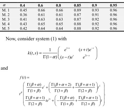
eigenvalues of stability matrix ℜ. Table 1 shows the values of λ for methods 1-5, and different values of .α This insures us that the numerical solution of the corresponding methods is convergent to the exact solution, for given examples.
Table 1.
1,2,3 max ,
i i
λ λ
=
= for methods 1-5 and different values ofα .
α 0.4 0.6 0.8 0.85 0.9 0.95
M. 1 0.45 0.66 0.66 0.89 0.93 0.96
M. 2 0.36 0.61 0.61 0.87 0.91 0.96
M. 3 0.41 0.63 0.63 0.87 0.92 0.96
M. 4 0.43 0.65 0.65 0.88 0.92 0.96
M. 5 0.42 0.64 0.64 0.88 0.92 0.96
Now, consider system (1) with
2
( )
1 ( , )
(1 ) ( )
t s s
s t s
e s t e
k t s
s t e e
α
+ −
−
+ =
Γ − −
and
2
2
( )
( ) ( 2) ( 1)
(1 ) (3 ) (2 )
.
( 1) ( ) ( 1)
(2 ) (1 ) (2 )
t t
f t
e t
t
te t
β
β α β α β α
β β β
β α β α β α
β β β
=
Γ + + Γ + + +Γ + +
Γ + Γ + Γ +
Γ + + + −Γ + +Γ + +
Γ + Γ + Γ +
Then, the exact solution of the two dimensional system (1) is
(
1)
( ) s , s T.
y s = e s− β α+ − e sβ α+
We can construct the following examples by altering the parameters of the above system.
Example 7. 1. Let T =1, β =1 and 2 4, , 5 5
α= then apply the methods 1-3.
Example 7. 2. Let T =5, β =1 and 17 18 19, , , 20 20 20 α= then apply the methods 4-5.
Example 7. 3. Let T =10, β =1,1.5, 2 and α=0.9, then apply the methods 1-5.
By Theorem 5.2, we expect the error estimate
, 1 ,
( )
, ,
1
r
h
m
m
N r
e t c
m
N r
α
α
α β −
−
≤ ≤ ≤
≥ + −
‖ ‖
in Examples 7.1.-7.2. Tables, 2-5 confirm this error estimate.
Table 2. The absolute error and corresponding convergent order in Example 1 with r=1.
N α=0.4 α=0.8
M. 1 εN ρN εN ρN
N α=0.4 α=0.8
128 7.868e-3 0.388 3.697e-4 0.787
256 5.987e-3 0.394 2.132e-4 0.794
M. 2
N ε
N
ρ εN ρN
64 1.153e-2 - 4.989e-4 -
128 8.768e-3 0.395 2.878e-4 0.794
256 6.657e-3 0.397 1.656e-4 0.797
M. 3
N ε
N
ρ εN ρN
64 1.227e-2 - 4.694e-4 -
128 9.320e-3 0.396 2.705e-4 0.795
256 7.072e-3 0.398 1.556e-4 0.798
Table 3. The absolute error and corresponding convergent order in Example
1 with r 2
α = .
N α=0.4 α=0.8
M. 1
N ε
N
ρ εN ρN
64 1.177e-4 - 2.789e-5 -
128 2.978e-5 1.983 7.240e-6 1.946
256 7.492e-6 1.991 1.880e-6 1.946
M. 2
N ε
N
ρ εN ρN
64 1.299e-4 - 1.551e-5 -
128 3.421e-5 1.925 3.938e-6 1.978
256 8.776e-6 1.963 9.924e-7 1.989
M. 3
N ε
N
ρ εN ρN
64 1.624e-4 - 2.558e-5 -
128 4.325e-5 1.908 6.798e-6 1.912
256 1.120e-5 1.949 1.781e-6 1.932
Table 4. The absolute error and corresponding convergent order in Example
2 with r =1.
N α=0.85 α=0.95
M. 4
N ε
N
ρ εN ρN
32 3.281e-4 - 3.763e-5 -
64 1.750e-4 0.907 1.759e-5 1.097
128 9.689e-5 0.853 8.867e-6 0.988
M. 5
N ε
N
ρ εN ρN
32 4.236e-4 - 4.435e-5 -
64 2.281e-4 0.893 2.024e-5 1.132
128 1.259e-4 0.858 1.014e-5 0.997
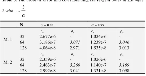
Table 5. The absolute error and corresponding convergent order in Example
2 with r 3
α = .
N α=0.85 α=0.95 M. 1
N ε
N
ρ εN ρN
32 2.677e-6 - 1.024e-6 -
64 3.186e-7 3.071 1.239e-7 3.046
128 4.064e-8 2.971 1.535e-8 3.013
M. 2
N ε
N
ρ εN ρN
32 2.359e-6 - 1.026e-6 -
64 2.463e-7 3.260 1.140e-7 3.169
128 2.992e-8 3.041 1.331e-8 3.098
Also, by Theorem 5.2, we expect the estimate
( 0.1)
, 1 ,
0.1 ( )
, ,
1
r
h
m
m
N r
e t c
m
N r
β
β
α β − −
−
≤ ≤ − ≤
≥ + −
‖ ‖
in Example 7.3. Tables, 6-7 show this estimate. In all tables, we reported estimate of the order for the component of the system which is less. Finally, these examples show that the obtained convergent result is optimal and can’t be improved for our investigated class of SWSVIEFKs.
Table 6. The absolute error and corresponding convergent order in Example
3 with r = 1
N β=1 β=2
M. 1
N ε
N
ρ εN ρN
256 1.635e-4 - 5.918e-5 -
512 8.873e-5 0.882 1.601e-5 1.886
M. 2 256 1.179e-4 - 2.732e-5 -
512 6.362e-5 0.890 7.496e-6 1.866
M. 3 256512 1.079e-4 5.821e-5 - 0.890 1.986e-5 5.334e-6 - 1.897
M. 4 256 3.494e-5 - 7.828e-7 -
512 1.874e-5 0.899 2.131e-7 1.877
M. 5 256 1.858e-5 - 4.904e-7 -
512 9.943e-6 0.902 1.337e-7 1.875
Table 7. The absolute error and corresponding convergent order in Example
3 with
0.1
r
m
β
= − .
N β=1 β=2
M. 1
N ε
N
ρ εN ρN
128 8.908e-7 - 1.597e-5 -
256 2.112e-7 2.077 4.126e-6 1.953
M. 2 128256 7.452e-6 1.891e-6 - 1.978 6.391e-5 1.641e-5 - 1.962
M. 3 128 1.373e-5 - 1.053e-4 -
256 3.710e-6 1.888 2.854e-5 1.883
M. 4 128 5.925e-8 - 1.697e-7 -
256 8.340e-9 2.829 2.135e-8 2.990
M. 5 128 5.925e-8 - 1.697e-7 -
256 8.340e-9 2.829 2.135e-8 2.990
8. Conclusion
A convergence analysis of the collocation methods for SWSVIEFKs on discontinuous piecewise polynomial spaces has been investigated. Based on this analysis, the order of the method does not change by increasing collocation parameters on uniform mesh. However, it can be increased up to m by using graded mesh. Our analysis stands on the eigenvalues of stability matrix. We obtained a closed form of this eigenvalues for case
1.
m= However, for cases m>1,we obtained the eigenvalues of stability matrix for prescribed collocation parameters.
References
[1] K. E. Atkinson, “The numerical solution of integral equations of the second kind,” Vol. 4, Cambridge university press, 1997. [2] H. W. Branca, “The nonlinear Volterra equation of abel's kind
and its numerical treatment,” Comput, 1978, 20, 307-324. [3] H. Brunner, “Collocation methods for Volterra integral and