http://www.sciencepublishinggroup.com/j/acm doi: 10.11648/j.acm.20170606.12
ISSN: 2328-5605 (Print); ISSN: 2328-5613 (Online)
A Comparative Study on Fourth Order and Butcher’s Fifth
Order Runge-Kutta Methods with Third Order Initial Value
Problem (IVP)
Md. Babul Hossain
1, *, Md. Jahangir Hossain
2, Md. Musa Miah
1, Md. Shah Alam
11
Department of Mathematics, Mawlana Bhashani Science and Technology University, Tangail-1902, Bangladesh 2Department of Basic Science, World University of Bangladesh, Dhaka, Bangladesh
Email address:
[email protected] (Md. B. Hossain) *Corresponding author
To cite this article:
Md. Babul Hossain, Md. Jahangir Hossain, Md. Musa Miah, Md. Shah Alam. A Comparative Study on Fourth Order and Butcher’s Fifth Order Runge-Kutta Methods with Third Order Initial Value Problem (IVP). Applied and Computational Mathematics.
Vol. 6, No. 6, 2017, pp. 243-253. doi: 10.11648/j.acm.20170606.12
Received: September 26, 2017; Accepted: October 8, 2017; Published: November 8, 2017
Abstract:
In this paper, Butcher’s fifth order Runge-Kutta (RK5) and fourth order Runge-Kutta (RK4) methods have been
employed to solve the Initial Value Problems (IVP) involving third order Ordinary Differential Equations (ODE). These two
proposed methods are quite proficient and practically well suited for solving engineering problems based on such problems. To
obtain the accuracy of the numerical outcome for this study, we have compared the approximate results with the exact results
and found a good agreement between the exact and approximate solutions. In addition, to achieve more accuracy in the
solution, the step size needs to be very small. Moreover, the error terms have been analyzed for these two methods and also
compared by an appropriate example.
Keywords:
Differential Equation, Initial Value Problem, Error, Butcher’s Method, Runge-Kutta Method
1. Introduction
Most of the branches in science, economics, management,
engineering etc. most problems are formulated by differential
equations. Most of the equations do not have analytical
solutions, adequate to the development of numerical
techniques. To solve these problems numerical approximations
are convenient. For finding numerical approximations many
methods are developed. Initial Value Problem (IVP) and
Boundary Value Problem (BVP) are two parts of differential
equations, depending on the conditions indicated at the end
points of the domain. There are many methods that yield
approximate solutions of initial value problems of Ordinary
Differential Equations (ODE), such as Euler’s method
developed by Leonhard Euler in 1768, Runge-Kutta method
developed around 1900 by Carl Runge and Martin Wilhelm
Kutta respectively. Many authors try to spread these methods
to get higher accurate solution of Initial Value Problems (IVP).
In [1] the author presented fifth order improved Runge-Kutta
method for solving ordinary differential equation, in [2] the
author presented on fifth order Runge-Kutta methods, also in
[3] the author presented a comparative study on numerical
solutions of Initial Value Problems (IVP) for Ordinary
Differential Equations (ODE) with Euler and Runge-Kutta
methods. Also in [4] – [15] presented various numerical
methods for finding approximations of Initial Value Problems
(IVP) in Ordinary Differential Equations (ODE).
In this paper, we converted the coefficients of Butcher’s
RK5 table to the general fifth order Runge-Kutta method.
Also we use fourth order Runge-Kutta (RK4) and fifth order
Runge-Kutta (RK5) methods for solving third order initial
value
problems
in
ordinary
differential
equations.
Approximate results are compared to the exact results and
compared between these two methods.
2. Numerical Methods
differential equations (ODEs). Next we will apply these two
methods for solving third order initial value problem.
2.1. Runge-Kutta Method
Runge-Kutta method is a technique for approximating the
solution of ordinary differential equation. This technique was
developed around 1900 by mathematicians Carl Runge and
Wilhelm Kutta. Runge-Kutta method is popular because of
its relative simplicity, sufficiency, accuracy and efficiency
and used in most computer programs for a differential
equation. This method is distinguished by their order in the
sense that agrees with Taylor’s series solution up to terms of
ℎ
where is the order of the method.
2.2. Runge-Kutta Fourth Order Method
Consider the following initial value problem:
=
,
(1)
with initial condition
=
.
Now the method is based on computing
as follows:
=
+
+ 2 + 2 +
(2)
where
=
+ ℎ
=
,
=
+
ℎ
2 , +
ℎ
2
=
+
ℎ
2 , +
ℎ
2
=
+ ℎ, + ℎ
For
= 0, 1, 2, … … … …
2.3. Fourth Order Runge-Kutta Method for Solving Initial
Value Problem (IVP) for the System of Three
Differential Equations
Consider the following system of differential equations:
= ! ", , , #
(3)
= $ ", , , #
(4)
%
= & ", , , #
(5)
with initial conditions
" = , " =
# " = # .
The fourth order Runge-Kutta method will become as:
(
=
(+
) * + ,(6)
(
=
(+
-) -* -+ -,(7)
#
(= #
(+
.) .* .+ .,(8)
Where
"
(= "
(+ ℎ
= ! "
(,
(,
(, #
(/ = $ "
(,
(,
(, #
(0 = & "
(,
(,
(, #
(= ! "
(+
ℎ
2 ,
(+
2 ,
ℎ
(+
ℎ
2 / , #
(+
ℎ
2 0
/ = $ "
(+
ℎ
2 ,
(+
2 ,
ℎ
(+
ℎ
2 / , #
(+
ℎ
2 0
0 = & "
(+
ℎ
2 ,
(+
2 ,
ℎ
(+
ℎ
2 / , #
(+
ℎ
2 0
= ! "
(+
ℎ
2 ,
(+
2 ,
ℎ
(+
ℎ
2 / , #
(+
ℎ
2 0
/ = $ "
(+
ℎ
2 ,
(+
ℎ
2 ,
(+
ℎ
2 / , #
(+
ℎ
2 0
0 = & "
(+
ℎ
2 ,
(+
2 ,
ℎ
(+
ℎ
2 / , #
(+
ℎ
2 0
= ! "
(+ ℎ,
(+ ℎ ,
(+ ℎ/ , #
(+ ℎ0
/ = $ "
(+ ℎ,
(+ ℎ ,
(+ ℎ/ , #
(+ ℎ0
0 = & "
(+ ℎ,
(+ ℎ ,
(+ ℎ/ , #
(+ ℎ0
For
1 = 0, 1, 2, … … … ..
2.4. Butcher’s Fifth Order Runge-Kutta Method
Consider the following initial value problem:
=
,
(9)
with initial condition
=
.
Now the method is based on computing
as follows:
=
+
27 + 32 + 12 + 32
5+ 7
(10)
Where
=
+ ℎ
=
,
=
+
1
4 ℎ, +
1
4 ℎ
=
+
1
4 ℎ, +
1
8 ℎ +
1
8 ℎ
5
=
+
3
4 ℎ, +
16 ℎ +
3
16 ℎ
9
=
+ ℎ, −
3
7 ℎ +
2
7 ℎ +
12
7 ℎ −
12
7 ℎ +
8
7
5ℎ
For
= 0, 1, 2, … … … ….
2.5. Butcher’s Fifth Order Runge-Kutta Method for Solving
Initial Value Problem (IVP) for the System of Three
Differential Equations
Assume that the following system of differential
equations:
= ! ", , , #
(11)
= $ ", , , #
(12)
%
= & ", , , #
(13)
with initial conditions
" = , " = ,
# " = # .
The Butcher’s fifth order Runge-Kutta method will
become as:
(
=
(+
90 7 + 32 + 12 + 32
ℎ
5+ 7
(
=
(+
90 7/ + 32/ + 12/ + 32/
ℎ
5+ 7/
#
(= #
(+
90 70 + 320 + 120 + 320
ℎ
5+ 70
where
"
(= "
(+ ℎ
= ! "
(,
(,
(, #
(/ = $ "
(,
(,
(, #
(0 = & "
(,
(,
(, #
(= ! "
(+
1
4 ℎ,
(+
4 ℎ,
1
(+
1
4 / ℎ, #
(+
1
4 0 ℎ
/ = $ "
(+
1
4 ℎ,
(+
4 ℎ,
1
(+
1
4 / ℎ, #
(+
1
4 0 ℎ
0 = & "
(+
1
4 ℎ,
(+
4 ℎ,
1
(+
1
4 / ℎ, #
(+
1
4 0 ℎ
= ! "
(+
1
4 ℎ,
(+
1
8 ℎ +
1
8 ℎ,
(+
1
8 / ℎ +
1
8 / ℎ, #
(+
1
8 0 ℎ +
1
8 0 ℎ
/ = $ "
(+
1
4 ℎ,
(+
1
8 ℎ +
1
8 ℎ,
(+
1
8 / ℎ +
1
8 / ℎ, #
(+
1
8 0 ℎ +
1
8 0 ℎ
0 = & "
(+
1
4 ℎ,
(+
1
8 ℎ +
1
8 ℎ,
(+
1
8 / ℎ +
1
8 / ℎ, #
(+
1
8 0 ℎ +
1
8 0 ℎ
= ! "
(+
1
2 ℎ,
(−
1
2 ℎ + ℎ,
(−
1
2 / ℎ + / ℎ, #
(−
1
2 0 ℎ + 0 ℎ
/ = $ "
(+
1
2 ℎ,
(−
1
2 ℎ + ℎ,
(−
1
2 / ℎ + / ℎ, #
(−
1
2 0 ℎ + 0 ℎ
0 = & "
(+
1
2 ℎ,
(−
1
2 ℎ + ℎ,
(−
1
2 / ℎ + / ℎ, #
(−
1
2 0 ℎ + 0 ℎ
5
= ! "
(+
3
4 ℎ,
(+
16 ℎ +
3
16 ℎ,
9
(+
16 / ℎ
3
+
16 / ℎ, #
9
(+
16 0 ℎ +
3
16 0 ℎ
9
/
5= $ "
(+
3
4 ℎ,
(+
16 ℎ +
3
16 ℎ,
9
(+
16 / ℎ
3
+
16 / ℎ, #
9
(+
16 0 ℎ +
3
16 0 ℎ
9
0
5= & "
(+
3
4 ℎ,
(+
16 ℎ +
3
16 ℎ,
9
(+
16 / ℎ
3
+
16 / ℎ, #
9
(+
16 0 ℎ +
3
16 0 ℎ
9
= ! "(+ ℎ, (−37 ℎ +27 ℎ +127 ℎ −127 ℎ +87 5ℎ, (
−37 / ℎ +27 / ℎ +127 / ℎ −127 / ℎ +87 /5ℎ,
#
(−
;0 ℎ +
;0 ℎ +
;0 ℎ −
;0 ℎ +
<;0
5ℎ
)
/ = $ "(+ ℎ, (−37 ℎ +27 ℎ +127 ℎ −127 ℎ +87 5ℎ, (
−37 / ℎ +27 / ℎ +127 / ℎ −127 / ℎ +87 /5ℎ,
#
(−
;0 ℎ +
;0 ℎ +
;0 ℎ −
;0 ℎ +
<;0
5ℎ
)
0 = & "(+ ℎ, (−37 ℎ +27 ℎ +127 ℎ −127 ℎ +87 5ℎ, (
−37 / ℎ +27 / ℎ +127 / ℎ −127 / ℎ +87 /5ℎ,
#
(−
;0 ℎ +
;0 ℎ +
;0 ℎ −
;0 ℎ +
<;0
5ℎ
)
For
1 = 0, 1, 2, 3, … … … …
3. Error Analysis
limited number of significant figures. Thus, such numbers
cannot be represented exactly in computer memory. The
discrepancy introduced by this limitation is called Round-off
error. Truncation error in numerical analysis arises when
approximations are used to estimate some quantity. The
accuracy of the solution will depend on how small we take
the step size
ℎ
. A numerical method is said to be convergent
if the numerical solution approaches the exact solution as the
step size
ℎ
goes to 0. In this paper, we consider a third order
initial value problem to verify accuracy of the proposed
method. Then using this method we find numerical
approximations for desired initial value problems. The
approximate solution is evaluated by using MATLAB
software for two proposed numerical methods at different
step sizes. The convergence of initial value problem is
calculated by
=
>= |# "
>− #
>| < A
where
# "
>denotes the
approximate solution and
#
>denotes the exact solution and
A
depends on the problem which varies from
10
B. The errors
for these two formulas are defined by
= C D = |# "
>− #
>|
.
4. Applications of These Numerical
Methods on Illustrative Example
In this section we consider a third order initial value
problem as numerical example to compare between these two
methods. All the computations are performed by MATLAB
software. Numerical results and errors are computed and the
outcomes are represented by graphically.
Example:
Consider the initial value problem
+%+− 5
**%+ 8
%−
4# = 0
with initial conditions
# 0 = 1, #
F0 = 2, #
FF0 =
−1
on the interval
0 ≤ " ≤ 3
. The exact solution of the given
problem is
# " = −5=
+ 6 − 5" =
.
Now this third order initial value problem can be written in
the form of system of first order differential equations by
putting
=
%and
=
=
*%*as
%
=
(14)
=
(15)
= 5 − 8 + 4#
(16)
with initial conditions
# 0 = 1, 0 = 2
and
0 = −1
.
The approximate results, exact results and maximum errors
for step sizes 0.1, 0.05, 0.025 and 0.0125 are shown in Table
1-4 and the graphs of the numerical solutions.
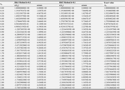
Table 1. Numerical approximations and maximum errors for step size h=0.1.
HI RK4 Method h=0.1 RK5 Method h=0.1 Exact value J
I
J HI errors J HI errors
0.00 1.000000000E+00 0.0000E+00 1.000000000E+00 0.0000E+00 1.000000000E+00
0.10 1.191879167E+00 1.8587E-05 1.191860509E+00 7.0649E-08 1.191860580E+00
0.20 1.352158372E+00 4.8675E-05 1.352109515E+00 1.8279E-07 1.352109697E+00
0.30 1.450335750E+00 9.5186E-05 1.450240210E+00 3.5363E-07 1.450240564E+00
0.40 1.443205050E+00 1.6482E-04 1.443039619E+00 6.0647E-07 1.443040226E+00
0.50 1.270646705E+00 2.6666E-04 1.270379073E+00 9.7266E-07 1.270380046E+00
0.60 8.501696545E-01 4.1289E-04 8.497552721E-01 1.4942E-06 8.497567663E-01
0.70 6.985621392E-02 6.1983E-04 6.923415278E-02 2.2270E-06 6.923637976E-02
0.80 -1.220730555E+00 9.0924E-04 -1.221643039E+00 3.2453E-06 -1.221639794E+00
0.90 -3.222234415E+00 1.3099E-03 -3.223549006E+00 4.6473E-06 -3.223544359E+00
1.00 -6.200492971E+00 1.8601E-03 -6.202359606E+00 6.5622E-06 -6.202353043E+00
1.10 -1.050571353E+01 2.6098E-03 -1.050833253E+01 9.1599E-06 -1.050832337E+01
1.20 -1.659695942E+01 3.6252E-03 -1.660059728E+01 1.2663E-05 -1.660058461E+01
1.30 -2.507335987E+01 4.9925E-03 -2.507836972E+01 1.7361E-05 -2.507835236E+01
1.40 -3.671382206E+01 6.8245E-03 -3.672067024E+01 2.3634E-05 -3.672064661E+01
1.50 -5.252748238E+01 9.2684E-03 -5.253678271E+01 3.1972E-05 -5.253675074E+01
1.60 -7.381770747E+01 1.2515E-02 -7.383026553E+01 4.3015E-05 -7.383022252E+01
1.70 -1.022631744E+02 1.6813E-02 -1.022800447E+02 5.7590E-05 -1.022799871E+02
1.80 -1.400204583E+02 2.2482E-02 -1.400430174E+02 7.6764E-05 -1.400429407E+02
1.90 -1.898536787E+02 2.9939E-02 -1.898837199E+02 1.0192E-04 -1.898836179E+02
2.00 -2.552981612E+02 3.9719E-02 -2.553380155E+02 1.3483E-04 -2.553378806E+02
2.10 -3.408668260E+02 5.2513E-02 -3.409195170E+02 1.7777E-04 -3.409193392E+02
2.20 -4.523102017E+02 6.9209E-02 -4.523796445E+02 2.3370E-04 -4.523794108E+02
2.30 -5.969436997E+02 9.0949E-02 -5.970349547E+02 3.0637E-04 -5.970346483E+02
2.40 -7.840591906E+02 1.1920E-01 -7.841787876E+02 4.0060E-04 -7.841783870E+02
2.50 -1.025442174E+03 1.5583E-01 -1.025598527E+03 5.2258E-04 -1.025598004E+03
2.60 -1.336021133E+03 2.0325E-01 -1.336225064E+03 6.8020E-04 -1.336224383E+03
2.70 -1.734682248E+03 2.6453E-01 -1.734947664E+03 8.8354E-04 -1.734946780E+03
2.80 -2.245290896E+03 3.4360E-01 -2.245635639E+03 1.1455E-03 -2.245634493E+03
2.90 -2.897971535E+03 4.4545E-01 -2.898418468E+03 1.4824E-03 -2.898416986E+03
Table 2. Numerical approximations and maximum errors for step size h=0.05.
HI RK4 Method h=0.05 RK5 Method h=0.05 Exact value J
I
J HI errors J HI errors
0.00 1.000000000E+00 0.0000E+00 1.000000000E+00 0.0000E+00 1.000000000E+00
0.10 1.191861879E+00 1.2998E-06 1.191860576E+00 3.0532E-09 1.191860580E+00
0.20 1.352113095E+00 3.3976E-06 1.352109690E+00 7.8667E-09 1.352109697E+00
0.30 1.450247197E+00 6.6333E-06 1.450240549E+00 1.5162E-08 1.450240564E+00
0.40 1.443051695E+00 1.1470E-05 1.443040200E+00 2.5913E-08 1.443040226E+00
0.50 1.270398578E+00 1.8532E-05 1.270380005E+00 4.1429E-08 1.270380046E+00
0.60 8.497854265E-01 2.8660E-05 8.497567028E-01 6.3461E-08 8.497567663E-01
0.70 6.927935934E-02 4.2980E-05 6.923628542E-02 9.4337E-08 6.923637976E-02
0.80 -1.221576807E+00 6.2986E-05 -1.221639931E+00 1.3714E-07 -1.221639794E+00
0.90 -3.223453694E+00 9.0665E-05 -3.223544555E+00 1.9595E-07 -3.223544359E+00
1.00 -6.202224407E+00 1.2864E-04 -6.202353319E+00 2.7612E-07 -6.202353043E+00
1.10 -1.050814302E+01 1.8035E-04 -1.050832375E+01 3.8469E-07 -1.050832337E+01
1.20 -1.660033426E+01 2.5035E-04 -1.660058514E+01 5.3085E-07 -1.660058461E+01
1.30 -2.507800780E+01 3.4455E-04 -2.507835308E+01 7.2660E-07 -2.507835236E+01
1.40 -3.672017589E+01 4.7072E-04 -3.672064759E+01 9.8758E-07 -3.672064661E+01
1.50 -5.253611181E+01 6.3893E-04 -5.253675207E+01 1.3341E-06 -5.253675074E+01
1.60 -7.382936022E+01 8.6230E-04 -7.383022431E+01 1.7924E-06 -7.383022252E+01
1.70 -1.022788292E+02 1.1579E-03 -1.022799895E+02 2.3966E-06 -1.022799871E+02
1.80 -1.400413930E+02 1.5476E-03 -1.400429438E+02 3.1906E-06 -1.400429407E+02
1.90 -1.898815579E+02 2.0601E-03 -1.898836222E+02 4.2312E-06 -1.898836179E+02
2.00 -2.553351487E+02 2.7320E-03 -2.553378862E+02 5.5912E-06 -2.553378806E+02
2.10 -3.409157287E+02 3.6106E-03 -3.409193466E+02 7.3647E-06 -3.409193392E+02
2.20 -4.523746540E+02 4.7569E-03 -4.523794205E+02 9.6720E-06 -4.523794108E+02
2.30 -5.970283993E+02 6.2490E-03 -5.970346610E+02 1.2668E-05 -5.970346483E+02
2.40 -7.841701997E+02 8.1873E-03 -7.841784036E+02 1.6549E-05 -7.841783870E+02
2.50 -1.025587304E+03 1.0700E-02 -1.025598026E+03 2.1570E-05 -1.025598004E+03
2.60 -1.336210431E+03 1.3953E-02 -1.336224411E+03 2.8054E-05 -1.336224383E+03
2.70 -1.734928626E+03 1.8155E-02 -1.734946817E+03 3.6412E-05 -1.734946780E+03
2.80 -2.245610919E+03 2.3575E-02 -2.245634540E+03 4.7172E-05 -2.245634493E+03
2.90 -2.898386430E+03 3.0556E-02 -2.898417047E+03 6.1003E-05 -2.898416986E+03
3.00 -3.731247292E+03 3.9534E-02 -3.731286905E+03 7.8758E-05 -3.731286826E+03
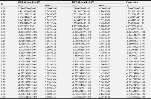
Table 3. Numerical approximations and maximum errors for step size h=0.025.
HI RK4 Method h=0.025 RK5 Method h=0.025 Exact value J
I
J HI errors J HI errors
0.00 1.000000000E+00 0.0000E+00 1.000000000E+00 0.0000E+00 1.000000000E+00
0.10 1.191860665E+00 8.5920E-08 1.191860579E+00 1.1046E-10 1.191860580E+00
0.20 1.352109922E+00 2.2438E-07 1.352109697E+00 2.8413E-10 1.352109697E+00
0.30 1.450241002E+00 4.3772E-07 1.450240563E+00 5.4680E-10 1.450240564E+00
0.40 1.443040982E+00 7.5632E-07 1.443040225E+00 9.3328E-10 1.443040226E+00
0.50 1.270381267E+00 1.2212E-06 1.270380045E+00 1.4903E-09 1.270380046E+00
0.60 8.497586539E-01 1.8876E-06 8.497567640E-01 2.2803E-09 8.497567663E-01
0.70 6.923920903E-02 2.8293E-06 6.923637637E-02 3.3862E-09 6.923637976E-02
0.80 -1.221635649E+00 4.1443E-06 -1.221639799E+00 4.9180E-09 -1.221639794E+00
0.90 -3.223538396E+00 5.9629E-06 -3.223544366E+00 7.0206E-09 -3.223544359E+00
1.00 -6.202344586E+00 8.4570E-06 -6.202353053E+00 9.8849E-09 -6.202353043E+00
1.10 -1.050831152E+01 1.1853E-05 -1.050832338E+01 1.3761E-08 -1.050832337E+01
1.20 -1.660056817E+01 1.6447E-05 -1.660058463E+01 1.8976E-08 -1.660058461E+01
1.30 -2.507832973E+01 2.2629E-05 -2.507835238E+01 2.5956E-08 -2.507835236E+01
1.40 -3.672061570E+01 3.0906E-05 -3.672064664E+01 3.5256E-08 -3.672064661E+01
1.50 -5.253670880E+01 4.1939E-05 -5.253675078E+01 4.7598E-08 -5.253675074E+01
1.60 -7.383016593E+01 5.6587E-05 -7.383022258E+01 6.3914E-08 -7.383022252E+01
1.70 -1.022799111E+02 7.5965E-05 -1.022799872E+02 8.5414E-08 -1.022799871E+02
1.80 -1.400428391E+02 1.0151E-04 -1.400429408E+02 1.1366E-07 -1.400429407E+02
1.90 -1.898834828E+02 1.3510E-04 -1.898836181E+02 1.5065E-07 -1.898836179E+02
2.00 -2.553377015E+02 1.7913E-04 -2.553378808E+02 1.9899E-07 -2.553378806E+02
2.10 -3.409191026E+02 2.3669E-04 -3.409193395E+02 2.6200E-07 -3.409193392E+02
2.20 -4.523790990E+02 3.1178E-04 -4.523794112E+02 3.4395E-07 -4.523794108E+02
2.30 -5.970342388E+02 4.0951E-04 -5.970346488E+02 4.5030E-07 -5.970346483E+02
2.40 -7.841778506E+02 5.3645E-04 -7.841783876E+02 5.8808E-07 -7.841783870E+02
2.50 -1.025597303E+03 7.0101E-04 -1.025598005E+03 7.6623E-07 -1.025598004E+03
2.60 -1.336223469E+03 9.1396E-04 -1.336224384E+03 9.9620E-07 -1.336224383E+03
2.70 -1.734945591E+03 1.1890E-03 -1.734946781E+03 1.2926E-06 -1.734946780E+03
2.80 -2.245632949E+03 1.5438E-03 -2.245634495E+03 1.6741E-06 -2.245634493E+03
2.90 -2.898414985E+03 2.0008E-03 -2.898416988E+03 2.1643E-06 -2.898416986E+03
Table 4. Numerical approximations and maximum errors for step size h=0.0125.
HI RK4 Method h=0.0125 RK5 Method h=0.0125 Exact value J
I
J HI errors J HI errors
0.00 1.000000000E+00 0.0000E+00 1.000000000E+00 0.0000E+00 1.000000000E+00
0.10 1.191860585E+00 5.5223E-09 1.191860579E+00 3.7019E-12 1.191860580E+00
0.20 1.352109712E+00 1.4415E-08 1.352109697E+00 9.5168E-12 1.352109697E+00
0.30 1.450240592E+00 2.8110E-08 1.450240564E+00 1.8304E-11 1.450240564E+00
0.40 1.443040274E+00 4.8553E-08 1.443040226E+00 3.1220E-11 1.443040226E+00
0.50 1.270380124E+00 7.8375E-08 1.270380046E+00 4.9825E-11 1.270380046E+00
0.60 8.497568874E-01 1.2111E-07 8.497567662E-01 7.6200E-11 8.497567663E-01
0.70 6.923656123E-02 1.8148E-07 6.923637965E-02 1.1311E-10 6.923637976E-02
0.80 -1.221639528E+00 2.6576E-07 -1.221639794E+00 1.6421E-10 -1.221639794E+00
0.90 -3.223543977E+00 3.8230E-07 -3.223544359E+00 2.3434E-10 -3.223544359E+00
1.00 -6.202352501E+00 5.4210E-07 -6.202353044E+00 3.2983E-10 -6.202353043E+00
1.10 -1.050832261E+01 7.5963E-07 -1.050832337E+01 4.5902E-10 -1.050832337E+01
1.20 -1.660058356E+01 1.0539E-06 -1.660058461E+01 6.3280E-10 -1.660058461E+01
1.30 -2.507835091E+01 1.4498E-06 -2.507835236E+01 8.6533E-10 -2.507835236E+01
1.40 -3.672064463E+01 1.9798E-06 -3.672064661E+01 1.1751E-09 -3.672064661E+01
1.50 -5.253674805E+01 2.6862E-06 -5.253675074E+01 1.5861E-09 -5.253675074E+01
1.60 -7.383021889E+01 3.6240E-06 -7.383022252E+01 2.1294E-09 -7.383022252E+01
1.70 -1.022799822E+02 4.8644E-06 -1.022799871E+02 2.8451E-09 -1.022799871E+02
1.80 -1.400429342E+02 6.4998E-06 -1.400429407E+02 3.7851E-09 -1.400429407E+02
1.90 -1.898836093E+02 8.6494E-06 -1.898836179E+02 5.0163E-09 -1.898836179E+02
2.00 -2.553378692E+02 1.1467E-05 -2.553378806E+02 6.6247E-09 -2.553378806E+02
2.10 -3.409193241E+02 1.5151E-05 -3.409193393E+02 8.7195E-09 -3.409193392E+02
2.20 -4.523793909E+02 1.9955E-05 -4.523794108E+02 1.1443E-08 -4.523794108E+02
2.30 -5.970346221E+02 2.6209E-05 -5.970346483E+02 1.4976E-08 -5.970346483E+02
2.40 -7.841783527E+02 3.4330E-05 -7.841783870E+02 1.9552E-08 -7.841783870E+02
2.50 -1.025597959E+03 4.4858E-05 -1.025598004E+03 2.5466E-08 -1.025598004E+03
2.60 -1.336224325E+03 5.8480E-05 -1.336224383E+03 3.3100E-08 -1.336224383E+03
2.70 -1.734946704E+03 7.6076E-05 -1.734946780E+03 4.2936E-08 -1.734946780E+03
2.80 -2.245634394E+03 9.8770E-05 -2.245634493E+03 5.5591E-08 -2.245634493E+03
2.90 -2.898416858E+03 1.2799E-04 -2.898416986E+03 7.1851E-08 -2.898416986E+03
3.00 -3.731286660E+03 1.6558E-04 -3.731286826E+03 9.2713E-08 -3.731286826E+03
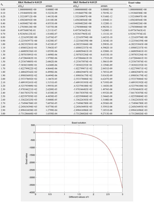
Figure 2. Approximate numerical solutions.
Figure 4. Error for step size h=0.05.
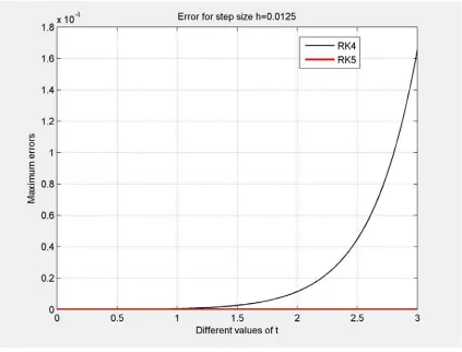
Figure 6. Error for step size h=0.0125.
Figure 8. Error for different step sizes using RK5 method.
5. Discussion
The acquired results are displayed in Tables 1-4 and
graphically presented in Figures (1-8). The approximate
solutions and maximum errors are calculated with the step
sizes 0.1, 0.05, 0.025 and 0.0125 and also compared to the
exact solutions. Also from Tables 1-4 we observe that RK5
method gives more accurate results and better than RK4
method. This argument is also cleared by Figures 3-6. From
all Tables and Figures for each method we say that a
numerical solution converges to the exact solution if the step
size is decreased. Also from figures 7 and 8 we conclude that
if the step size tends to zero then the errors also tends to zero.
6. Conclusion
In this paper, fourth order Runge-Kutta method and
Butcher’s fifth order Runge-Kutta method are applied to
solve third order initial value problem (IVP) of ordinary
differential equation (ODE). To find more accurate results
we reduced the step size for both the methods. From the
resulting tables and figure we have analyzed that the
solutions of both methods are converges to the exact
solutions for decreasing the step size
ℎ
. From the figure 2
we see that both methods give almost same results but from
figures 3-6 it is clear that RK5 method gives more accurate
results than RK4 method. We state that the Butcher’s fifth
order Runge-Kutta method is more appropriate and
proficient for finding the numerical solutions of initial
value problems (IVP) than fourth order Runge-Kutta
method. Hence from this study it is clear that to find more
accurate results higher order methods are appropriate than
lower order methods.
References
[1] Rabiei, F., & Ismail, F. (2012). Fifth-order Improved Runge-Kutta method for solving ordinary differential equation. Australian Journal of Basic and Applied Sciences, 6 (3), 97-105.
[2] Butcher, J. C. (1995). On fifth order Runge-Kutta methods. BIT Numerical Mathematics, 35 (2), 202-209.
[3] Islam, M. A. (2015). A Comparative Study on Numerical Solutions of Initial Value Problems (IVP) for Ordinary Differential Equations (ODE) with Euler and Runge-kutta Methods. American Journal of Computational Mathematics, 5 (03), 393.
[4] Butcher, J. C. (1964). On Runge-Kutta processes of high order. Journal of the Australian Mathematical Society, 4 (02), 179-194.
[5] Butcher, J. C. (1996). A history of Runge-Kutta methods. Applied numerical mathematics, 20 (3), 247-260.
[7] Goeken, D., & Johnson, O. (2000). Runge–Kutta with higher order derivative approximations. Applied numerical mathematics, 34 (2-3), 207-218.
[8] Lambert, J. D. (1973). Computational methods in ordinary differential equations. Wiley, New York.
[9] Hall, G. and Watt, J. M. (1976) Modern Numerical Methods for Ordinary Differential Equations. Oxford University Press, Oxford.
[10] Mathews, J. H. (2005) Numerical Methods for Mathematics, Science and Engineering. Prentice-Hall, India.
[11] Gerald, C. F. and Wheatley, P. O. (2002) Applied Numerical Analysis. Pearson Education, India.
[12] Burden, R. L. and Faires, J. D. (2002) Numerical Analysis. Bangalore, India.
[13] Sastry, S. S. (2000) Introductory Methods of Numerical Analysis. Prentice-Hall, India.
[14] Balagurusamy, E. (2006) Numerical Methods. Tata McGraw-Hill, New Delhi.