Transformations of summary statistics as input in meta-analysis for linear dose-response models on a logarithmic scale: a methodology developed within EURRECA

R E S E A R C H A R T I C L E

Open Access

Transformations of summary statistics as input in

meta-analysis for linear dose

–

response models on

a logarithmic scale: a methodology developed

within EURRECA

Olga W Souverein

, Carla Dullemeijer

, Pieter van `t Veer

and Hilko van der Voet

Abstract

Background:To derive micronutrient recommendations in a scientifically sound way, it is important to obtain and analyse all published information on the association between micronutrient intake and biochemical proxies for micronutrient status using a systematic approach. Therefore, it is important to incorporate information from randomized controlled trials as well as observational studies as both of these provide information on the association. However, original research papers present their data in various ways.

Methods:This paper presents a methodology to obtain an estimate of the dose–response curve, assuming a bivariate normal linear model on the logarithmic scale, incorporating a range of transformations of the original reported data. Results:The simulation study, conducted to validate the methodology, shows that there is no bias in the

transformations. Furthermore, it is shown that when the original studies report the mean and standard deviation or the geometric mean and confidence interval the results are less variable compared to when the median with IQR or range is reported in the original study.

Conclusions:The presented methodology with transformations for various reported data provides a valid way to estimate the dose–response curve for micronutrient intake and status using both randomized controlled trials and observational studies.

Keywords:Methodology, Dose–response, Meta-analysis, EURRECA

Background

Meta-analysis of the association between micronutrient intake and biochemical proxies for micronutrient status or function is needed when setting micronutrient recom-mendations. Information on this association may come from randomized controlled trials as well as from obser-vational studies. In a randomized trial subjects are ran-domized to receive either the intervention treatment or the control treatment, and a meta-analysis of such stud-ies will usually provide a mean difference in micronu-trient status between placebo and intervention groups, answering the question whether the biochemical status marker responds to the dietary intake of a micronutrient

[1-3]. However, this analysis does not provide an esti-mate of the slope of the dose–response relationship. On the other hand, a meta-analysis of observational studies provides an estimate of the slope of the dose–response relation, but observational studies are hampered by for instance measurement error in the intake estimates, which causes bias in the reported association [4-6].

Ideally, information from observational studies and rando-mized controlled trials should be compared or even com-bined in a single meta-analysis to ensure that all reported information is taken into account over a broad range of in-take. This requires that the summary statistics reported in individual studies are transformed into estimates of the dose–response relation. Since both intake and status are continuous variables, this estimate is actually an estimate of the regression coefficient of the linear regression of micronu-trient status on micronumicronu-trient intake. The individual

* Correspondence:[email protected] 1

Division of Human Nutrition, Wageningen University and Research Centre, P.O. Box 8129, 6700, EV Wageningen, the Netherlands

Full list of author information is available at the end of the article

estimates of the dose–response regression coefficient may then be combined in a meta-analysis.

The statistical combination of study results may be com-plicated by the variety of ways that individual studies re-port the summary statistics. The results from randomized controlled trials as well as the baseline summary statistics of micronutrient intake and status may be reported as means, medians or geometric means. Variability is often reported as standard deviations, standard errors, inter-quartile ranges (IQR), ranges or confidence intervals (CI). In observational studies the relation between intake and status can be reported as a Pearson correlation coefficient, a Spearman rank correlation coefficient or a regression co-efficient. In addition, either the intake variable or the sta-tus variable or both could have been logarithmically transformed before the correlation or association was cal-culated. All these different ways of reporting need to be standardized before meta-analysis is even possible.

This paper gives an overview of transformation meth-ods to algebraically derive an estimate from each study of the regression coefficient (slope, b) and its standard error (se(b)), for studies that do not directly report these. The methods are validated by comparing the cal-culated values with theoretical values in a small-scale simulation study.

Methods

In order to derive transformations we assume a bivariate normal distribution on the log-scale for intake and

status of an individual person. The log-scale was chosen because both intake and status values are always above zero, and the observed distributions of the micronu-trient variables are often right-skewed. Moreover, as the true shape of the dose–response curve is usually un-known the linear relation between logarithmically trans-formed quantities provides the simplest approximation. More in detail, for the dose–response meta-analysis of observational studies we assume that ξ0 (intake of

micronutrient) and η₀ (status or continuous health out-come) are log-normally distributed. The assumption of bivariate normality entails a linear association between ξ¼ lnð Þξ0 and η¼ ln η0 , where ln denotes the natural

logarithm. Note that we use the Greek lettersξandηfor the theoretical values of intake and status/response, and the Latin letters X and Y for the observed values of these variables. Furthermore, we reserve letters without sub-script (e.g. X and Y) for values expressed on the ln-scale, and use letters with subscript 0 (e.g., X0 and Y0) for values expressed on the absolute (i.e., original) scale.

The process of data transformations to obtain the required statistics from what is reported in observational studies, consists of four steps (Figure 1). The first step is to obtain the mean of X (mX) and Y (mY) and the standard deviation of X (sX) and Y (sY). Secondly, the mean of X0 (mX0) and Y0 (mY0) and the standard deviation of X0 (sX0) and Y0(sY0) are calculated when needed for the cal-culations in step 3. In this third step the correlation coeffi-cient of the association between X and Y (rXY) is

Step 1

Calculate mX, sX and mY, sY from reported univariate statistic using equations (1)-(7)

Step 2

Calculate mX0, sX0 and mY0, sY0 from

mX, sX and mY, sY: equations (8), (9)

Step 3

Calculate rXY from reported bivariate statistic using equations (10)-(17)

Step 4

Calculate bYX from rXY: equation (18)

Calculate se(bYX): equation (19)

OBSERVATIONAL STUDIES RANDOMIZED CONTROLLED _TRIALS

Step 1

Calculate mY and sY from reported values after intervention for placebo and intervention group using equations (1)-(7)

Step 2

Calculate mX as ln(mX0) for both

placebo and intervention group

Step 3

Calculate bYX: equation (20) Calculate se(bYX): equation (21)

calculated from the reported data. In the last step, the re-gression coefficient of the linear rere-gression from Y on X (bYX) is calculated from rXY, and the se(bYX) is calculated from rXY, sY, sX and the sample size (n). For reports on randomized controlled trials, the process consists of three steps. In the first step, mY and sY are obtained for both intervention and placebo group. In the second step, mX is obtained, and in the last step, bYX and se(bYX) are calcu-lated. The equations for all these transformations are given below.

Univariate transformations

First, we describe how the univariate statistics of the nor-mal distributions at the ln-scale can be obtained from various reported statistics. We present formulas for mX and sX, which of course can also be used similarly for mY and sY in observational studies. For randomized con-trolled trials the situation is different, because the vari-ation in X is artificial and is not described by a normal distribution. Therefore, the transformations should be used only to obtain mY and sY in the intervention and placebo groups separately. In most trials the within-group variation in X will be ignorable compared with the difference between the groups, consequently mX is cal-culated simply as mXcon= ln(mX0_con) for the placebo group and as mXint= ln(mX0_int) the intervention group.

For these transformations, we assume that ξ is normally distributed with parametersμ_ξandσξ. For a lognormal

dis-tribution the mean on the absolute scale, μ_ξ0, is given by μξ0¼ exp μξþ0:5σ

2

ξ

and the standard deviation on the

absolute scale, σξ0, is given by σξ0 ¼ exp μξþ0:5σ

2

ξ

ffiffiffiffiffiffiffiffiffiffiffiffiffiffiffiffiffiffiffiffiffiffiffiffiffiffiffi

exp σ2

ξ 1 r

. It follows that when the mean (mX0) and

the standard deviation (sX0) are reported, mX can be calcu-lated as:

mX¼lnðmX₀Þ 0:5sX2 _ð1Þ

where

sX¼

ffiffiffiffiffiffiffiffiffiffiffiffiffiffiffiffiffiffiffiffiffiffiffiffiffiffiffiffiffiffiffiffiffiffiffiffiffiffi

ln 1þ sX0 mX0

2!

v u u

t _ð2Þ

The exponential function of the mean of the lognormal distribution is equal to the median on the absolute scale. Therefore, when the median (medX0) has been reported on the absolute scale, mX is calculated as:

mX¼lnðmedX₀Þ ð3Þ

As a measure of variability an IQRx or range (rangex) is often reported together with the median or mean. The IQR is the difference between the third quartile Q3 and

first quartile Q1(the 75thpercentile and the 25th percent-ile). Basically, there are two cases. If the lower and upper limits are reported as such, the difference between the ln-transformed limits may be equated to an appropriate multiple of the standard deviation sX. On the other hand, if only the IQR or range is reported as such, the derivation is more complex. When IQRX0 is reported together with the median, the relation between

these and sX is given by IQRX0¼medX0

exp zð sXÞ expðzsXÞ

½ , where z represents the

ap-propriate percentage point in the standard normal distri-bution (i.e., z0.75= 0.6745).

In this case sX may be calculated as

sX¼ ln 1

2 IQRX0

medX0þ

ffiffiffiffiffiffiffiffiffiffiffiffiffiffiffiffiffiffiffiffiffiffiffiffiffiffi

IQRX0

medX0 2

þ4

r !

" #

z ð4Þ

When the IQR is reported together with the mean no explicit formula exists to derive sX. Therefore, to obtain an estimate of sX from these quantities a nonlinear func-tion optimizafunc-tion is employed to find the value of sX for which the following equation holds

IQRX₀¼mX0 exp 0:5sX2

½exp zð sXÞ expðzsXÞ: ð5Þ

When the lower and upper bounds of the IQR (i.e., Q1 (X0) and Q3(X0) respectively) are reported, rather than the difference, sX may be calculated as sX¼½Q3ð Þ X Q1ð ÞX =2z:

The range is the difference between the maximum and the minimum value of the data. Equations (4) and (5) may be similarly used when the range is reported, but here we consider that the minimum and the maximum represent the lower and upper (1/n) fraction of the data-set of n observations. Therefore we expect a fraction p = 1-1/(2n) below the minimum and the same fraction above the maximum, and in the equations above we need to use zp. For example, in a dataset with n = 100 we use z0.995= 2.576.

The geometric mean (gm) of the lognormal distribu-tion is equal to exp(mX), and is most often reported in papers together with the 95% confidence limits. mX and sX are obtained for these quantities using:

mX¼lnðgmX₀Þ; ð6Þ

sX¼pffiffiffin ln X0;upp

ln X0;low

2z0:975 ð

7Þ

Then in step 2 for observational studies, mx and sx are calculated in case these estimates were not already avail-able. These statistics at the original scale may be needed in the bivariate transformations described below. The equations are:

mX0¼expðmXþ0:5sX2Þ ð8Þ

sX0¼mX0

ffiffiffiffiffiffiffiffiffiffiffiffiffiffiffiffiffiffiffiffiffiffiffiffiffiffiffi

exp sX 2₁

q

ð9Þ

Bivariate transformations (to obtain regression or correlation coefficients)

For observational studies, the next step is to obtain an estimate of the correlation between X and Y (rXY). The equations below can be used to obtain rXY from reported correlation and regression coefficients taking into account the possibility that either X0, log10(X0), X, Y0, log10(Y0) or Y was used for the originally reported statistic.

When a study reports the association as a Spearman rank correlation coefficient (rS), rXY is calculated as

rXY¼rs ð10Þ

Another option is that the association between X0and Y0 is reported as a regression coefficient (bY0X0). In that case the correlation coefficient, rX0Y0, is calculated first using

rX0Y0¼bY0X0

sX0

sY0 ð

11Þ

and then rXY is calculated using the following equation which was derived from Johnson & Kotz [7]:

rXY¼

ln 1þrX0Y0

ffiffiffiffiffiffiffiffiffiffiffiffiffiffiffiffiffiffiffiffiffiffiffiffiffiffiffiffiffiffiffiffiffiffiffiffiffiffiffiffiffiffiffiffiffiffiffiffiffiffiffiffiffiffiffiffiffiffiffiffiffiffiffiffiffiffiffi exp sX 2_{1 exp sY} 2₁

q

n o

sXsY

ð12Þ

This formula (12) is also used when the Pearson prod-uct–moment correlation coefficient rX0Y0 is directly reported in a paper.

For observational studies that report the regression co-efficient between Y0 and X, the correlation coefficient, rXY0, is calculated using

rXY0¼bY0X

sX

sY0 ð

13Þ

When log10(X0) is used instead of X, sX is replaced by sX/ln(10) in formula (13).

Then rXY is calculated using the following equation [8,9]:

rXY¼rXY0

ffiffiffiffiffiffiffiffiffiffiffiffiffiffiffiffiffiffiffiffiffiffiffiffiffiffiffiffiffiffiffi

exp sY 2₁

q

sY ð14Þ

This formula (14) is also used when rXY0 is reported directly or when the Pearson product–moment correl-ation coefficient is reported between log10(X0) and Y0.

When the regression coefficient between Y and X0 is reported in an observational study, the regression coeffi-cient, rX0Y, is calculated using

rX0Y¼bYX0

sX0

sY ð15Þ

When log10(Y0) is used instead of Y, sY is replaced by sY/ln(10) in formula (15).

Using rX0Y or the directly reported Pearson product– moment correlation coefficient between X0and log10(Y0) or Y in an observational study, rXY is calculated using [8,9]:

rXY¼rX0Y

ffiffiffiffiffiffiffiffiffiffiffiffiffiffiffiffiffiffiffiffiffiffiffiffiffiffiffiffiffiffiffi

exp sX 2₁

q

sX ð16Þ

When the regression coefficient between X and Y is reported, rXY is calculated as

rXY¼bYXsX

sY ð17Þ

Calculation of dose–response regression coefficient In the last step, for both observational studies and rando-mized controlled trials, we need to obtain bYX and se(bYX). For observational studies, the required regression coefficient bYX is calculated from the correlation coefficient:

bYX¼rXYsY

sX ð18Þ

and the corresponding standard error (se(bYX)) is calcu-lated as

seðbYXÞ ¼

ffiffiffiffiffiffiffiffiffiffiffiffiffiffiffiffiffiffiffiffiffiffiffiffiffiffiffiffiffiffiffiffiffiffiffiffi

sY21rXY2 N2

ð Þ sX2

s

ð19Þ

For randomized controlled trials, the required regres-sion coefficient bYX is calculated as:

bYX¼ mYintmYcon

mXintmXcon ð

20Þ

se bYXð Þ ¼

ffiffiffiffiffiffiffiffiffiffiffiffiffiffiffiffiffiffiffiffiffiffiffiffiffiffiffiffiffiffiffiffiffiffiffiffiffiffiffiffiffiffiffiffiffiffiffiffiffiffiffiffiffiffiffiffiffiffiffiffiffiffiffiffiffiffiffiffiffiffiffiffiffiffiffiffiffiffiffiffiffiffiffiffiffiffiffiffiffiffiffiffiffiffiffiffiffiffiffiffiffiffiffiffiffiffiffiffiffiffiffiffiffiffiffiffiffiffiffiffiffiffiffiffiffiffiffiffiffiffiffiffiffiffiffiffiffiffiffiffiffiffiffiffiffiffiffiffiffiffiffiffiffiffiffiffiffiffiffiffiffiffiffiffiffiffiffiffiffiffiffiffiffi

Ncon1

ð Þ sYcon2þðNint1Þ sYint2

NconþNint2

ð Þ

1

Nconþ

1 Nint

1

mXintmXcon

ð Þ2

! v

u u

t _ð21Þ

Simulation study

A simulation study was conducted to validate the per-formance of the transformations given in this paper. Bi-variate lognormal data (X,Y) were simulated where X ~ Normal(1.60,0.852) and Y ~ Normal(5.70,0.452). Par-ameter values were based on values of vitamin B12 in-take (X) and serum/plasma vitamin B12 (Y) [10-13]. Different strengths of the correlation between X and Y were simulated, namely 0.1, 0.5 and 0.9.

A sample of individuals (with sample size 100, 200 or 500) was randomly drawn, and values that represent differ-ent often used reporting options were calculated from this sample, namely the mean and SD, the median and IQR, the median and range and the geometric mean and 95% CI (all summary statistics on the absolute scale). Also, the correl-ation and regression coefficients of X and Y expressed in different scales were calculated. These ‘reported’ values were rounded to two decimal places. From these‘reported’ values, the parameter estimates mX, mY, sX, sY and rXY were calculated using the transformations described in this paper. This process was repeated 1000 times.

Results

Table 1 shows the simulation results for the univariate statistics. On average the calculated values of mX and mY are almost the same as the true values, indicating that no important bias is present in these calculations. As expected, the 95% CI of the simulations is smaller for the simulations with a sample size of 500 than for the

simulations with a sample size of 200 or 100. For sX and sY, the estimates are most precise when a geometric mean with a 95% CI is reported, and least precise when a median with a range is reported.

Figure 2 shows the simulation results when a correlation coefficient is reported, and Figure 3 shows the simulation results when a linear regression coefficient is reported. Both these figures show the simulation results with true rXY = 0.5. Results are similar for true rXY = 0.9 and true rXY = 0.1 (data not shown). For the situation in which a correlation coefficient is the reported bivariate statistic, there is no difference for the four univariate reporting options. Therefore, these results are pooled in Figure 2.

None of the combinations of univariate and bivariate reporting options shows evidence of bias with the average of the simulations almost equal to the true value. The width of the confidence interval indicates the variability of the simulations. Because there is no appreciable bias, a smaller CI width indicates that the individual simulations are closer to the true correlation. The accuracy is best when rX0Y is reported and worst when rX0Y0 is reported. As expected, the accuracy is also better when the sample size is larger. Figure 3 shows that the CI is wider when the reported uni-variate statistics are the median and IQR or median and range. The larger variation in the results for the transform-ation from bYX0(Figure 3B) compared with the variation in the results from bY0X (Figure 3C) is caused by the fact the X was simulated with larger standard deviation than Y.

Table 1 Simulation results for mX, sX, mY and sY

n mX sX mY sY

True 1.6 0.85 5.7 0.45

Mean, SD 100 1.6 (1.4-1.8) 0.82 (0.65-1.06) 5.7 (5.6-5.8) 0.45 (0.37-0.53)

200 1.6 (1.4-1.7) 0.83 (0.70-1.03) 5.7 (5.6-5.8) 0.45 (0.40-0.51)

500 1.6 (1.5-1.7) 0.84 (0.75-0.98) 5.7 (5.7-5.7) 0.45 (0.42-0.49)

Median, IQR 100 1.6 (1.4-1.8) 0.84 (0.63-1.10) 5.7 (5.6-5.8) 0.44 (0.35-0.56)

200 1.6 (1.5-1.8) 0.85 (0.70-1.02) 5.7 (5.6-5.8) 0.45 (0.38-0.53)

500 1.6 (1.5-1.7) 0.85 (0.76-0.95) 5.7 (5.7-5.7) 0.45 (0.40-0.50)

Median, range 100 1.6 (1.4-1.8) 0.83 (0.58-1.14) 5.7 (5.6-5.8) 0.44 (0.32-0.60)

200 1.6 (1.5-1.8) 0.83 (0.63-1.12) 5.7 (5.6-5.8) 0.44 (0.35-0.58)

500 1.6 (1.5-1.7) 0.83 (0.68-1.06) 5.7 (5.7-5.7) 0.44 (0.36-0.56)

Gm, 95% CI 100 1.6 (1.4-1.8) 0.85 (0.73-0.97) 5.7 (5.6-5.8) 0.45 (0.38-0.51)

200 1.6 (1.5-1.7) 0.85 (0.77-0.94) 5.7 (5.6-5.8) 0.45 (0.41-0.49)

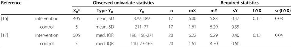
Example

To illustrate the methodology some examples of its use on real data for vitamin B12 are reported in Table 2

(observational studies [14,15]) and Table 3 (randomized controlled trials [16,17]). The tables show the statistics as reported in the studies and the statistics that are cal-culated using the different equations presented in this paper (which are entitled ‘required statistics’ in the tables).

Discussion

The investigated means, standard deviations, correlation coefficients and sample sizes were based on real-life values. The univariate statistics that are investigated in this paper were limited to mean and SD, median and IQR or range and geometric mean and 95% CI. These do not represent all reporting options that can be encountered in the literature, but cover most published papers. Other combinations of univariate statistics that were seen are for example mean with IQR, mean with range, and geometric mean with standard deviation. Also, the investigated regression and correlation coeffi-cients are limited in this paper to those on the absolute or logarithmic scale, whereas sometimes other transfor-mations to normality have been used in reports, such as a square root transformation. However, as the logarith-mic transformation is by far the most often used trans-formation in papers in the medical research area, the

A.

B.

D.

C.

Figure 3Simulation results for rXY from different reporting options where the true rXY was 0.5.A) b from linear regression of Y0on X0; B)

b from linear regression of Y on X0; C) b from linear regression of Y0on X; D) b from linear regression of Y on X and from the linear regression of

log10(Y0) on log10(X0). Circles indicate that the reported univariate statistic was mean + SD, squares indicate median and IQR, diamonds indicate

median and range, and triangles indicate geometric mean. Bars represent 95% confidence intervals. In each group the three bars from left to right are for sample sizes of 100, 200 and 500 individuals, respectively.

Figure 2Simulation results for rXY where the true rXY was 0.5.

Circles indicate that the reported bivariate statistic was rX0Y0, squares

indicate rXY0and diamonds indicate rX0Y. Bars represent 95%

equations in this paper will cover most published papers in this field.

The bivariate normal linear model on the logarithmic scale is an approximation that is used here because the data are positive data. Note that it allows the relation-ship between X0 and Y0 to be a linear, monotonic con-vex or monotonic concave function (i.e., for a slope equal, higher or lower than one, respectively). Even though some randomized controlled trials may investi-gate the dose–response relationship by providing mul-tiple dosages in their study, most of these studies include only one intervention and one control group and consequently it is often unknown what the true rela-tionship is. Therefore, this approximation provides a practical methodology to estimate the dose–response re-lationship and to combine the results from randomized controlled trials and observational studies. It was out-side the scope of the simulation study to investigate other shapes of the dose–response relation.

The transformations in this paper consider reported regression and correlation coefficients that are un-adjusted for other variables. It is possible to adjust the equations for adjusted regression or correlation coeffi-cients, if these adjustments were done on the log-scale. However, most often adjustment has been done on an-other scale, and moreover studies do not report all required statistics. Therefore, we did not consider adjusted coefficients.

In this paper we presented a methodology that allows for information from RCTs and observational studies to be summarised in comparable statistics. One possible application is to combine results of both types of study in a single meta-analysis. In general, a meta-analysis should include as much information as possible. How-ever, there may be systematic differences between

observational studies and randomized controlled trials. Therefore, it is advisable to check whether the size of the estimated regression coefficient differs between these dif-ferent study designs. This may be done by stratified ana-lysis or by using meta-regression techniques.

Conclusions

The presented methodology provides calculations to use results from published literature to estimate the slope of the dose–response relation incorporating information from both randomized controlled trials and observa-tional studies. The simulations clearly show that there is no observable bias associated with the transformations. Also, it can be seen that when a regression coefficient is reported, it is preferable to report the univariate statis-tics as mean and SD or geometric mean and 95% CI ra-ther than as median with IQR or range.

Abbreviations

b: Regression coefficient; CI: Confidence interval; gm: Geometric mean; IQR: Interquartile range; m: Mean; med: Median; r: Correlation coefficient; s: Standard deviation; se: Standard error.

Competing interests

The authors declare that they have no competing interests_’.

Authors’contributions

OS participated in the design of the simulation study, performed the statistical analysis and drafted the manuscript. CD helped to draft the manuscript and participated in the design of the simulation study. PvtV participated in the coordination of the study and revised the manuscript critically. HvdV conceived of the study, helped with the statistical analysis and interpretation of the and revised the manuscript critically. All authors read and approved the final manuscript.

Authors’information

OS and CD are both postdoctoral research fellows at the Division of Human Nutrition of Wageningen University, the Netherlands. PvtV is professor of Nutrition and Epidemiology at the Division of Human Nutrition, the Netherlands. HvdV is statistician at Biometris, Wageningen University and Research centre, the Netherlands.

Table 2 Example statistics for observational studies on vitamin B12 intake (X) and vitamin B12 status (Y)

Reference Observed univariate statistics Observed bivariate

statistic

Required statistics

Type X0and Y0 X0 Y0 n Association mX sX mY sY rXY bYX se(bYX)

[14] Mean, SD 9.3, 9.3 330, 140 177 rX0Y0 0.16 1.88 0.83 5.72 0.41 0.19 0.09 0.04

[15] gm, 95% CI 7.3, 7.1-7.5 354, 348-360 1329 rs 0.19 1.99 0.51 5.87 0.32 0.19 0.12 0.02

Table 3 Example statistics for randomized controlled trials on vitamin B12 intake and vitamin B12 status

Reference Observed univariate statistics Required statistics

X0* Type Y0 Y0 n mX mY sY bYX se(bYX)

[16] intervention 405 mean, SD 379, 189 17 6.00 5.83 0.47 0.12 0.03

control 5 mean, SD 211, 77 17 1.61 5.29 0.35

[17] intervention 505 med, IQR 198, 158-271 20 6.22 5.29 0.40 0.13 0.04

control 5 med, IQR 110, 73-165 20 1.61 4.70 0.60

*) X0represents the dose provided plus the dietary intake. When dietary intake of vitamin B12was not reported 5μg/day was added to the provided dose. The

Acknowledgements

We would like to thank the reviewer, Wolfgang Viechtbauer, for his valuable comments to the manuscript.

The work reported herein has been carried out within the EURRECA Network of Excellence (www.eurreca.org) which is financially supported by the Commission of the European Communities, specific Research, Technology and Development (RTD) Programme Quality of Life and Management of Living Resources, within the Sixth Framework Programme, contract no. 036196. This report does not necessarily reflect the Commission's views or its future policy in this area.

Author details 1

Division of Human Nutrition, Wageningen University and Research Centre, P.O. Box 8129, 6700, EV Wageningen, the Netherlands.2_Biometris,

Wageningen University and Research Centre, P.O. Box 100, 6700 AC Wageningen, the Netherlands.

Received: 3 January 2012 Accepted: 12 April 2012 Published: 25 April 2012

References

1. Hoey L, Strain JJ, McNulty H:Studies of biomarker responses to intervention with vitamin B-12: a systematic review of randomized controlled trials.Am J Clin Nutr2009,89:1981S–1996S.

2. Lowe NM, Fekete K, Decsi T:Methods of assessment of zinc status in humans: a systematic review.Am J Clin Nutr2009,89:2040S–2051S. 3. Ristic-Medic D, Piskackova Z, Hooper L, Ruprich J, Casgrain A, Ashton K,

Pavlovic M, Glibetic M:Methods of assessment of iodine status in humans: a systematic review.Am J Clin Nutr2009,89:2052S–2069S. 4. Kipnis V, Freedman LS:Impact of exposure measurement error in

nutritional epidemiology.J Natl Cancer Inst2008,100:1658–1659. 5. Kohlmeier L, Bellach B:Exposure assessment error and its handling in

nutritional epidemiology.Annu Rev Public Health1995,16:43–59. 6. Prentice RL:Dietary assessment and the reliability of nutritional

epidemiology research reports.J Natl Cancer Inst2010,102:583–585. 7. NLJohnsonSKotz1972Distributions in statistics: continuous multivariate distributionsWileyNew YorkJohnson NL, Kotz S:Distributions in statistics: continuous multivariate distributions. New York: Wiley; 1972.

8. Garvey PR:A family of joint probability models for cost and schedule uncertainties.27th Annual Department of Defense Cost Analysis Symposium September 19931993.

9. Yuan PT:On the logarithmic frequency distribution and the semi-logarithmic correlation.The Annals of Mathematical Statistics1933,4:30_–74. 10. Al Khatib L, Obeid O, Sibai AM, Batal M, Adra N, Hwalla N:Folate deficiency

is associated with nutritional anaemia in Lebanese women of childbearing age.Public Health Nutr2006,9:921–927.

11. Bates CJ, Schneede J, Mishra G, Prentice A, Mansoor MA:Relationship between methylmalonic acid, homocysteine, vitamin B12 intake and status and socio-economic indices, in a subset of participants in the British National Diet and Nutrition Survey of people aged 65 y and over.

Eur J Clin Nutr2003,57:349–357.

12. Hoey L, McNulty H, Askin N, Dunne A, Ward M, Pentieva K, Strain J, Molloy AM, Flynn CA, Scott JM:Effect of a voluntary food fortification policy on folate, related B vitamin status, and homocysteine in healthy adults.Am J Clin Nutr2007,86:1405–1413.

13. Shuaibi AM, Sevenhuysen GP, House JD:Validation of a food choice map with a 3-day food record and serum values to assess folate and vitamin B-12 intake in college-aged women.J Am Diet Assoc2008,108:2041_–2050. 14. Nath SD, Koutoubi S, Huffman FG:Folate and vitamin B12 status of a

multiethnic adult population.Journal of the National Medical Association

2006,98:67–72.

15. Vogiatzoglou A, Smith AD, Nurk E, Berstad P, Drevon CA, Ueland PM, Vollset SE, Tell GS, Refsum H:Dietary sources of vitamin B-12 and their association with plasma vitamin B-12 concentrations in the general population: the Hordaland Homocysteine Study.Am J Clin Nutr2009, 89:1078–1087.

16. Ubbink JB, Vermaak WJ, van der Merwe A, Becker PJ, Delport R, Potgieter HC:Vitamin requirements for the treatment of hyperhomocysteinemia in humans.The Journal of nutrition1994,124:1927–1933.

17. Yajnik CS, Lubree HG, Thuse NV, Ramdas LV, Deshpande SS, Deshpande VU, Deshpande JA, Uradey BS, Ganpule AA, Naik SS, Joshi NP, Farrant H, Refsum H:Oral vitamin B12 supplementation reduces plasma total homocysteine concentration in women in India.Asia Pacific journal of clinical nutrition

2007,16:103_–109.

doi:10.1186/1471-2288-12-57

Cite this article as:Souvereinet al.:Transformations of summary statistics as input in meta-analysis for linear dose–response models on a logarithmic scale: a methodology developed within EURRECA.BMC Medical Research Methodology201212:57.

Submit your next manuscript to BioMed Central and take full advantage of:

• Convenient online submission

• Thorough peer review

• No space constraints or color figure charges

• Immediate publication on acceptance

• Inclusion in PubMed, CAS, Scopus and Google Scholar

• Research which is freely available for redistribution