Real Securities Almgren

(1)

Chapter 2

Real Market Securities

So far, we have kept everything at a rather abstract level, remaining com-fortably in the realm of theoretical economics. Let’s look quickly at the real-world assets this theory is supposed to describe.

2.1 The basic assets

2.1.1 Stocks

A share of stock represents ownership of a piece of a corporation, called equity. Its value comes fundamentally from the real economic worth of the underlying operation over its whole future lifetime. Since this is very difficult to determine with any accuracy, the stock price is rather determined by what other people are willing to pay for it. This price fluctuates as popular opinion changes, and as news is revealed about the company and the environment.

The “efficient-market hypothesis” says that all information that any-one has about the value of the stock is reflected in the instantaneous stock price (for a popular account, see Malkiel). That is, if everyone be-lieves the price will go up later, they will start buying now and it will go up now. The main reason the price changes in the future is because of the random arrival of new information. Thus a random-walk model is the most logical for the motion of stock prices.

Note, however, that the fact that the changes in price themselves are unpredictable does not necessarily mean that theirstatistical properties are completely unpredictable. We may not be able to tell whether a stock will go up or down in the next half-hour (if we could do that consistently,

(2)

we could become very rich very quickly), but we may be able to guess, based on observation of past history, what theapproximate sizeof mo-tion we expect over a half-hour, over a day, or over a few months. It is this consistency that our mathematical techniques are based on. Thus, in our binomial tree models, we assumed we could decided in advance what thesetof possible paths was, though we had no idea and no opinion about which one would actually be chosen.

Of course, statistical consistency is possible only when no one is in a position to influence the statistic being measured. It is now possible to buy contracts on volatility itself, and it is possible that the existence and active trading of these products may change the behavior of the volatility used to model options.

2.1.2 Bonds and interest rates

Abondis a commitment to pay back a fixed amount of money at a fixed future date. Assuming the party making the commitment is reliable, the present value of this committment depends on the interest rate assumed to hold between now and the payment date. If interest rates rise, then bond prices fall.

In the last section, we assumed the existence of a single interest rate r, constant in time, at which we could borrow or lend money. But as anyone who has a credit card, a mortgage, a money market account, and a savings account knows, there is a wide variety of interest rates in the market.

Furthermore, interest rates change, in response to Alan Greenspan’s intervention or to market forces as with stocks. (My mortgage rate jumped up a quarter-point when Pat Buchanan won the 1996 New Hampshire Re-publican primary.)

In the context of pricing options on stocks, our answers to both these questions are influenced by the fact that stock motions are much more volatile than interest rate motions, so the time scales of interest in op-tion pricing are short compared to the times characterizing interest rate changes.

(3)

Robert Almgren Mathematics in Finance,Jan 11-12, 1999 27

The dynamics of long-term interest rates, and the pricing of deriva-tives on them, are an extremely interesting and mathematically challeng-ing area, which we will hear a little more about later in the course.

Another active area of much current research is the determination of spreads on corporate bonds, that is, the additional interest required to convince someone to lend to a company that has a nonnegligible risk of going bankrupt and being unable to repay.

2.1.3 Foreign exchange

All sorts of national currencies fluctuate against each other in response, as with stocks, to investors’ assessment of the relative desirablility of holding money in one country or another. Derivative contracts on foreign exchange can be priced using similar techniques as for derivatives on stocks. One difference is that account must be taken of the interest that can be earned by holding the foreign currentcy in comparison to the domestic.

2.2 Derivatives

Almost any contract that human imagination can invent is probably being bought and sold somewhere on the planet at this very moment. Let us focus our attention right now on the simplest, most important, and most widely traded derivative contracts.

2.2.1 Forwards and futures

Aforward contractis an agreement to buy a specific asset for a specified price, the strike price or delivery price, on a specified future expiration date. There is no optionality on either side: both parties are obligated to exchange cash and the asset when that date arrives, unless they sell the contract to someone else before then. Afutures contract is a highly stan-dardized version of a forward contract that can be traded on a exchange. The value of the forward contract at expiry is just the difference be-tween the price of the underlying asset at that time and the strike price. We write this as

(4)

-F_T

S_T F_T

S_T _K

K

[image:4.612.192.470.127.273.2]

Short Forward Long Forward

Figure 2.1: The payoff function at expiration time of a futures or forward contract with strikeK, as a function of the asset price at that time. On the left, the payoff to the person who is long the contract. On the right, the payoff to the person who is short, obviously the negative of the long position (since money is exchanged only between these two parties).

whereFT is the value of the contract at timeT, andST is the market price

of the underlying atT. Indeed, forward and futures contracts are often settled in cash rather than by actually exchanging the asset. This simple payoff functionis shown in Figure 2.1. (We shall use lettersF,C,P,etcto denote the price of specific derivatives such as forward contracts, calls, puts,etc;these correspond to theV of Chapter 1.)

The real question is, what should be the current priceF0of a forward contract? How much should you pay to sign up for this deal? Here we have the simplest example of risk-neutral pricing. Suppose thatS is the price per ounce of gold. Suppose someone offers you a forward contract to purchase one ounce of gold a timeT from now for a price K. What should you pay for this contract?

The first thing to figure out is whether the price of the contract de-pends on what you think the price of gold will do in the interval between now and T. You might think that the more likely the price is to rise, the greater the present priceF0 of the forward contract should be. But our discussion in Chapter 1 should have convinced you that subjective probabilities are often not important.

(5)

additional K cash, and you will be obliged to hand over one ounce of gold. You want to guarantee that you can do this, without incurring any risk because of possible motions of gold price between now and then.

The key is to buy the gold right now, and use bonds with guaranteed interest payments to take up any slack. So go buy one ounce of gold at the current price S0. Also, borrow Ke−r T dollars. At timeT, your customer gives you Kdollars which you use to exactly pay off your loan, and you give him the gold. The initial out-of-pocket cost to you of this strategy is S0−Ke−r T, and that is exactly the price you must demand from him:

F0 = S0 − K e−r T

If the forward contract is offered in the market at any different price than this, you can make a sure profit by running this cycle one way or the other.

In futures contracts, the delivery price is often determined so that no money changes hands now; K = er T_S₀ _so _F₀ ₌ _{0. The value} _K _{is the}

“future” price of the asset. Thus the futures price of an asset is simply a direct reflection of its present price, with slight modifications for interest costs.

This analysis assumes that the asset does not generate any return for the holder—a lump of gold, for example. If it is a stock that pays divi-dends, or a foreign currency that can be invested in the foreign country, then the above formula must be modified slightly.

2.2.2 Options

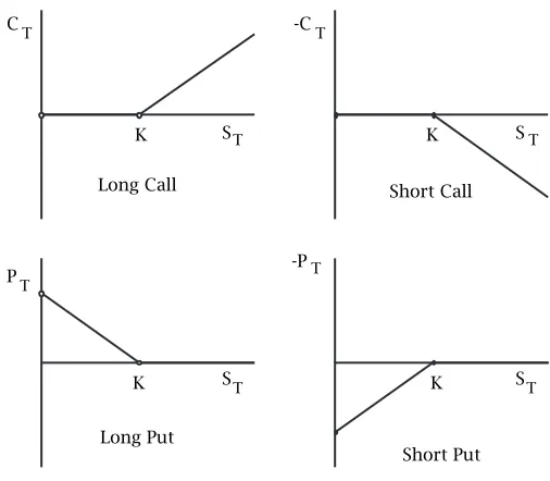
As its name implies, anoptiongives you, the holder, the choice whether to execute a certain transaction or not. Acall optiongives you the right to purchase a specified asset (from the counterparty: the person who sold you the option) for a specified price K, the strike price, at some future date or range of dates. Aput optiongives you the right to sell the asset (to the counterparty) for a specified strike priceK. Doing the purchase or the sale is calledexercising the option.

(6)

S_T S_T

-P_T P_T

-C_T

S_T C_T

S_T

K K

Short Put Long Put

[image:6.612.206.459.126.347.2]

Short Call Long Call

Figure 2.2: The values at expiry of vanilla call and put options, for both the long and the short side of the contract.

would lose money by purchasing the asset at priceK(since you can get it cheaper in the market), and the option expires worthless; it is out of the money. A put option is exactly the converse.

We know the values CT andPT at the expiry timet = T in terms of

the underlying asset priceST at that time:

Call: CT = maxST −K, 0

Put: PT = maxK−ST, 0 .

(Figure 2.2) Since the holder of the option always the freedom to tear it up and throw it out the window, its value is never negative. The short position is exactly opposite to the long position.

(7)

As outlined above, the most important purpose of “classical” financial mathematics is to determine the “correct” present value for a security, thusC0 andP0 for call and put options. Because the payoff functions in Figure 2.2 arenonlinear, the reasoning is more subtle than for forward contracts. We will need to use the full mechanisms of Chapter 1, together with refinements for continuous time that we explore in Chapter 3.

Options can be used tospeculate, meaning to take on additional risk in the hope of obtaining higher return. If you believe a certain stock is sure to go up, you can of course purchase the stock and hold it. But you can also purchase a call option on the stock for much less than the stock itself. Your gains are much amplified if the stock goes up. But if the stock closes the period below the strike price of the option (even if it goes up later) everything you spent for the option is lost.

Options can be used forhedging pre-existing risk. Almost all home mortgages are options on interest rates: you can refinance when you choose if rates drop, but are protected from rises in rates.

Options come in several different varieties. The most important dis-tinction is exactly when exercise is allowed. In Chapter 1, we have been implicitly been talking about Europeanoptions, which can be exercised on exactly one future date T, not before and not after. These can be valued in closed form, as we shall see later.

Most equity options areAmericanoptions, meaning that they can be exercised at any time (of the holder’s choice) before expiration. After the expiration date, they are worthless. Typical lifetimes for options are three, six, and nine months. Addition of the possibility of early exercise makes an American option always at least as valuable as its European counterpart. Pricing American options is more difficult than pricing Eu-ropean options.

Ordinary calls and puts are calledvanillaoptions to distinguish them from the myriad kinds ofexoticoptions with more complicated formulas. For example, Bermudan options (between American and European) can be exercised only on one of a set of prescribed dates before expiration. Asianoptions pay a value at expiration that depends on the average value of the asset price since the starting time. Lookback options pay a value that depends on the maximum or the minimum of the asset price over some specified period.

(8)

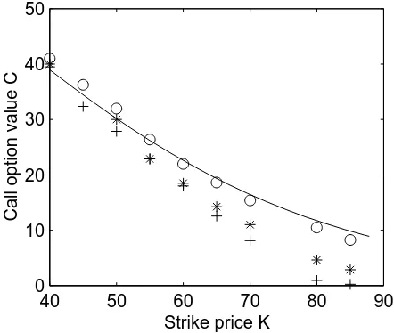
40 50 60 70 80 90 0

10 20 30 40 50

Strike price K

[image:8.612.220.440.134.321.2]

Call and put option value

Figure 2.3: Call (circle) and put (stars) option values on Dell Computer Corp, closing values on Friday, January 8, 1999. The lowest curve is January expiration, middle is February, and top is May. The straight solid lines areK−S andS−K.

price reaches the specified level before expiration.

Options and other derivatives are a way to trade risk between dif-ferent participants in the market. Common sense—this can be backed by classical economic theory based onPareto optimality—suggests that the more freedom people have to tailor their world, the better off they are. Indeed, when you insure your house, you are transferring risk to the insurance company. The probability and the cost of destruction do not change, but the company has a more robust risk appetite than an individ-ual (and in fact, the insurance company then redistributes the risk even more widely).

Of course, freedom to trade risk, like freedom to do anything else, can lead to problems. Recent well-publicized disasters (Orange County, MetalGesellschaft, Long-Term Capital Management) have illustrated the difficulty people can get themselves into in their search for profit.

(9)

all with the same strike K. It is clear by examining Figures 2.1 and 2.2 that at expiration, being long the call and short the put is equivalent to being long the foward, so

C − P = F.

Therefore, these two portfolios must have the same value at earlier times as well. Substituting the value of the forward contract, we have

C = P + S − Ke−r T

a time T before expiration. This formula is useful when the value of either a call or a put has been determined and the other one is desired.

A real example: Figure 2.3 shows some actual call and put option values (from the onlineWall Street Journal). Note that thex-axis in this picture is the strike price, not the stock price as in the other pictures (current stock price in this example isS0=7713/16=77.8). Thus the call option prices slope downwards: the less you want to be able to buy the asset for, the more you have to pay for the option.

(10)

(11)

Chapter 3

The Black-Scholes Equation

Hopefully these practical details will have whetted your appetite to return to the basic principles of no-arbitrage pricing, and to determine how to find fair values for complicated objects such as options at times before their expiration. To do this, we need to return to our tree, and figure out how to take it to a continuum limit.

3.1 Refining the tree

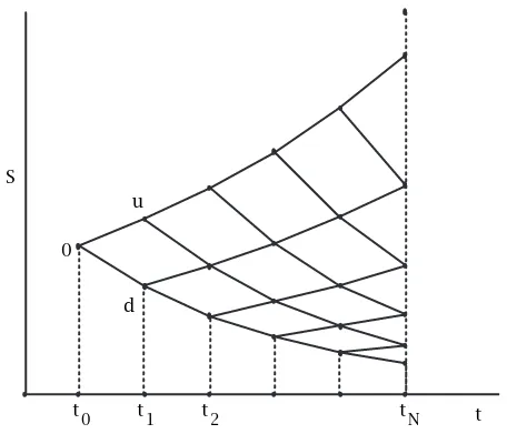
In Section 1.2, we constructed a tree havingN time steps. In the formu-lation there, N could be any number. For the given N, we were free to choose the 1₂(N+1)(N+2)stock valuesSijthat define the geometry of

the tree (we restrict ourselves to recombining trees). As long asS00=S0, the current stock price, we will come out with a value for the current option price, which hopefully will match what we read in the newspaper. Now, if the resulting value is to mean anything, it should not depend on the detailed properties of the tree, which is after all our own invention. At least, it should depend only on certain well-behaved properties of the tree, which we can correlate with properties of the stock we can observe in the real world.

Our overall strategy is the following: We are going to takeN → ∞, which means that our tree will be very closely sampled in time. As we do so, the number of nodes in each level will also go to∞, and we will make sure that as they do, they sample price space more and more finely. That is, the nodes will be closely spaced in both directions, and it is reasonable to hope that in the limit, the node values Vij will converge to a smooth

functionV (S, t).

(12)

S

t d

u

0

t_N t₂

[image:12.612.220.448.127.327.2]

t₁ t₀

Figure 3.1: A tree with constant up and down ratiosuandd.

This function will have terminal values V (S, T ) = Λ(S), the payoff function. The relationships between the valuesVijat neighboring nodes

on tree will approach apartial differential equation (PDE) relating local derivatives ofV(S, t). Then we will solve the equation to obtain the single value of interestV (S0,0), the current option price. Note that to obtain a picture such as Figure 2.3, we will have to repeat this procedure for eachdata point, each time taking a different payoff function (calls and puts with different strikes). This PDE will be the celebrated Black-Scholes equation, for which they got the Nobel prize.

In order to take the limitN→ ∞, we need to specify a regular structure for our tree (it would make no sense to construct it differently for each N). We need to specify a rule for determining the children Si+1,j and

Si+1,j+1in terms of each parent nodeSij. We shall do this by specifying

the up and downratiosuandd, rather than the differences:

Si+1,j = d Si,j, Si+1,j+1 = u Si,j.

The ratiosuanddwill be the same everywhere on the tree. In our model, therefore, in each time step the stock price can either gain a fixed per-centageor lose a fixed percentage. Figure 3.1 shows a tree with constant ratios.

(13)

example, if the initial price isS0 = $100, we might believe a reasonable motion is±$5 in one time interval. If this stock should hit a succession of “unlucky” moves, so that its price drops to $20, then the $5 intervals will start to look very large; we may prefer to believe that in that case the motions will become smaller in proportion.

It’s not very convincing to argue that one model is more plausible than another, since none of it yet appears very plausible at all. Perhaps a more convincing reason is that if we use constant increments, then for certain combinations of the initial price, the increment, and the number of steps, some of the prices on the leaves may become negative. Since a real stock price never becomes negative (even if the company goes bankrupt with lots of debt, the shareholders can just rip up their sharess), we will not know how to evaluate our derivative value in that event.

We do this in the following way. First, let us require that the time levels be equally spaced, with spacingk=T /N. Next, we pick a “spread” h, and a “centering term”s, and we define the up and down ratios to be

u = exphsk+ 1₂hi d = exphsk−1₂hi.

The reason for this choice is as follows:

• The ratio of the stock price at two successive nodes is u

d = eh,

so(u−d)/d≈h, andhdeserves to be called the spread.

• The geometric mean of the stock price at two successive nodes is p

ud = esk,

so the tree is “drifting” upwards at a fractional ratesper unit time. Note that each of these parameters is independent of the other. Both of them may depend onNand hencek.

Now,s has an action very similar to that of the interest rater. Since the interest rate played an important role in our pricing formula, we might expect that the relationship betweens andr will be important in this model.

Indeed, we must respect the inequality constraint that gives a positive pricing measure; here that requires

(14)

But, as long as this constraint is satisfied,swill not make any difference at all. We shall find that in the limitN→ ∞, the option price determined on the tree is controlledentirely byh.

Now let us return to our pricing formulas of Section 1.1.6. Applying (1.1) on our tree, with constant ratios S+/S0 = u and S−/S0 = d (and

T ,k), we find the pricing probability

q = er k−d u−d =

e(r−s)k₋_e−h/2

eh/2₋_e−h/2

the same at every node. Then we can directly apply the pricing formula (1.3),

Vi,j = e−r k

q Vi+1,j+1 + (1−q) Vi+1,j

(3.1)

(see Figure 3.2) one level at a time to computeVij on the whole tree. It

only remains to see what happens asN→ ∞, sok→0.

3.2 Continuum limit

We are almost done. In order to take the limit, we need only to specify how s and h behave as k → 0. We shall choose s to be constant as k decreases. As for h, we need it to go to zero along with k, so that our mesh yields nearly continuous price motions.

We shall choosehto vary so that

k = λ h2, λconstant ash→0.

(If you prefer, you can think of this as h = pk/λ.) It is not clear that this will be the right scaling. But if we do the computation with this scaling, we can explore other scalings by consideringλto be very large or very small. (For example, if you thought we should takek=ch, then I would argue that that is equivalent to settingλ=ch, so we can do the computation my way and then see what happens ifλis very small.)

(15)

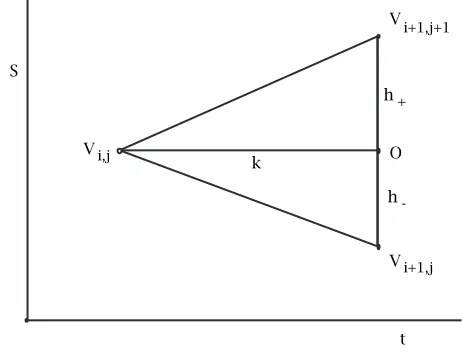
h₊

h -k

S

t O

V_i+1,j V_i+1,j+1

[image:15.612.165.396.131.312.2]

V_i,j

Figure 3.2: Expanding local values within one leaf of the tree.

The node valuesVij approach a smooth functionV (S, t)that

solves a partial differential equation. This PDE can be deter-mined by replacing the node values by the limit function eval-uated at the node points. The discrete relationship between node values will then no longer be exactly satisfied. Expand-ing everythExpand-ing in a local asymptotic series, and requirExpand-ing that the leading-order term vanish, gives the PDE.

In this case, we examine one leaf of the tree, that has the structure shown in Figure 3.2. The vertical lengths of the segments are

h+ = u−1S

h− = 1−dS,

whereS=Si,j, the vertical coordinate of pointO.

Following the prescription of finite-difference analysis, we suppose that the node values are given by samples of a smooth function, and we make the local asymptotic expansions

Vi,j = V − kvt + 1₂k2Vtt + · · ·

Vi+1,j = V − h−VS + 1₂h−2VSS + · · ·

(16)

where values ofV and derivatives that do not carry labels are evaluated at pointO.

Now all we have to do is plug these expansions into (3.1), expand everything in powers ofh, and see what the leading term in the error is. We shall spare you the details (the easiest is to toss everything into Mathematica) and just give the final result:

Vt + ₈1_λS2VSS + r SVS − r V = 0.

Of course, ash→0, the valuesVN,jtend smoothly to the valuesV (S, T ),

at expiration where the value is unambiguously known. This equation is backwards parabolicexcept possibly for some awkwardness nearS =0, so we have a completely defined problem for the option value: we solve the PDE and extract the valueV(S0,0).

Note that s has disappeared from the limiting PDE. What happens is thatq adjusts to exactly compensate for the drift term s. This fact is the reflection of what we have seen several times so far: if a price for a derivative can be obtained by arbitrage arguments, then it is of no significance what you believe the asset will do.

The limiting procedure we have employed is a little opaque for two reasons: first, because we have invoked results from finite difference analysis, and second, because we have skimmed over all the algebra. A simpler example may make the result clearer.

The pricing formula (3.1) essentially says that each node value Vi,j

is a sort of average of the two node values to its right. Of course q is not exactly 1₂, and there is the discount terme−r k_{, but essentially it is an}

average. So suppose thatr = 0 andq = 1₂, and let us suppose that we sets =0. In such a case it is not too hard to convince yourself that the result of this repeated averaging converges to a solution of the diffusion equation when the grid is refined. That’s the essence of this result.

Now we can return to a question we raised earlier: how did we know the scaling should be k ∼ λh2_{? We can answer this question by using} our knowledge of the diffusion equation:

1. Ifλ were extremely small, then the diffusion coefficient would be very large. The solutions would quickly reduce to constants. But option prices are demonstrably not constant functions.

(17)

equation, and its solutions would be translated and scaled copies of the terminal data. But option prices at times before expiry have a different shape than the payoff function; they are smoothed, as if by the action of a diffusive term.

Let us define a new parameterσ, thevolatility, by 1

8λ = 12σ2.

In other words, we specify that for a given k, our up and down steps should be chosen so that

h = 2σpk.

Then we can write the Black-Scholes equation in its standard form:

−Vt = 1₂σ2VSS + r SVS − r V int < T. (3.2)

with

V (S, T ) = Λ(S).

We have put the negative sign onVt because this equation isbackwards

parabolic: it is well-posed whenfinal data, rather than initial, is given. Let’s pause to think about what we have just derived. We have re-stricted our attention to European-style derivatives (no early exercise) with a finite upper time horizon at which the value is unambiguously known. For that type of problem, our assertion is that the value of any derivative security may be represented as a smooth function V (S, t) of time and of possible future asset prices S, satisfying the same univer-sal equation. Valuing a derivative then becomes a practical problem in solving an initial-value problem for a parabolic PDE.

But there’s a catch. For this argument to make sense, we need the result to be independent of the details of our discrete grid. But there is one parameter σ remaining in the final equation. Clearly the option value will depend on what value we pick forσ. We will see below thatσ is a measure of how much the stock price jumps around.

(18)

3.3 Solution of the Black-Scholes equation

We will not go through in detail the manipulations by which one obtains exact solutions to Equation (3.2); for sufficiently complicated problems one can bring to bear all the tricks and techniques available for solving parabolic equations in one dimension. We will only indicate the general method of solution, and give the two most famous solutions.

The first fact to notice is that (3.2) islinear and hasnonconstant co-efficients. The first fact is wonderful; in fact linear equations are the rule in finance rather than the exception.

The nonconstant coefficients are easily corrected. Since S appears only in the combinationS∂S, it is natural to change to a logarithmic

vari-able. Introduce new independent variables

x = log S

Sref, τ = σ

2_(T₋_t)

whereSrefis any reference price, and we are reversing and rescaling time only for convenience. Look for solutions in the form

V (S, t) = Vrefu

log S

Sref, σ

2_(T ₋_t)

whereu(x, τ) is a new dependent function, andVref is any convenient scale for the option value. Then (3.2) becomes

uτ = 1₂uxx + βux − γu,

in which the coefficients are

β = r −

1 2σ2

σ2 , γ =

r σ2.

We can easily solve this equation using Green’s functions.

In particular, the most famous solutions are those for the vanilla Eu-ropean call and put options. For a call with strike priceKwe have

C(S, t) = S N 

log(S/K)+

r+ 1₂σ2_(T₋_t)

σ√T−t

 

− K e−r (T−t)N 

log(S/K)+

r− 1₂σ2(T−t) σ√T−t

(19)

40 50 60 70 80 90

0 10 20 30 40 50

Strike price K

[image:19.612.168.389.135.322.2]

Call option value C

Figure 3.3: Comparison of the Black-Scholes formula with Dell call option prices from the newspaper. Circles are the May data against which the comparison is done. Volatility taken to beσ =0.6.

where N(·) is the cumulative normal distribution. The put value can be obtained by put-call parity. This formula is called the Black-Scholes formula.

Figure 3.3 shows a comparison of the “theoretical” value given by the Black-Scholes formula with the data from the Wall Street Journal for Dell call options. The traded options are actually American, whereas the explicit Black-Scholes formula applies only to Europeanoptions. In general, the possibility of early exercise increases the value of the option. But for a call option on an asset that does not pay dividends (or whose dividends can be neglected), exercise before expiry is never optimal and the American value is equal to the European one.

To evaluate the formula, we need values for all the parameters. Some are unambiguously known: S is the stock’s current price; Kis the inde-pendent variable, and r is the interest rate, typically 5 or 6 percent. I adjusted the volatilityσ to get a good fit. This graph is withσ = 0.6, a rather large value since this is a volatile stock. Withσ =0.6, the size of the expected changes in the course of one year are aboutσ2₌_36%.

(20)

40 50 60 70 80 90 0.5

0.6 0.7 0.8 0.9 1

Strike price K

Implied volatility

[image:20.612.218.442.132.319.2]

σ

Figure 3.4: Implied volatility for 5-month Dell calls.

we take the market prices as given, and determine the volatility indepen-dently for each different strike price (and each different maturity date) so as to reproduce that market price. This number is called theimplied volatility. Figure 3.4 shows the result.

In effect, we have traded one problem for another. We know the op-tion value in terms of the volatility, but we still need a value for the latter. Options are really ways to buy and sell volatility.

Although this data set does not show it very well, it is clear that the volatility that the market uses is larger when the spot price and the strike price are far apart. This is called the volatility smile and is present in all options markets. It indicates that the market’s assessment of the significance of large moves is greater than can be accounted for in the framework of the continuous-time limit of a binomial model.

3.4 Dynamic hedging

(21)

traded closes earlier than the option exchange) then mathematical theory saysnothing about the price of the option.

We discussed dynamic hedging in the discrete-time context in Chap-ter 1: the strategy was that you should hold∆units of the stock, where

∆ depended on what node you had reached in the evolution. As time evolved, and the price moved along its finite set of possible paths, you adjusted your holding with every change.

The exact value of∆was given in (1.4): ∆=(V2−V1)/(S2−S1). On the tree, subscripts 1 and 2 refer to two children of the same node, at the same time. Therefore, in the continuum limit, this ratio approaches the firstS-derivative ofV in the neighborhood of the nodes in question. Thus

∆ = ∂V ∂S.

As on the discrete tree, you have to solve the entire problem before you can find the initial value of∆.

As time evolves, the stock price will change as well. Unless the param-eters of the problem change, the functionV(S, t) will remain the same. But we must continuously adjust our hedge holdings to equal the value of∂V /∂S wherever we are on the tree at that time.

3.5 American options

All the analysis we have done so far is for European options. At each step, we have determined the arbitrage-free option value based on our holding it until the next time level.

If the option is American, then we have another possibility to con-sider. For each value of S andt, there is a payoff function Λ(S, t)that tells us how much we can get by exercising the option now. (For vanilla puts and calls, and many others, Λ is independent of t.) Certainly the value of the option can never be less than Λ, since we can exercise and get that amount. What do we do if the value predicted by the binomial formula is less than the value of early exercise?

(22)

first level of the iteration is exactly as before, since the terminal value is exactly the exercise value.

This may seem like not a valid strategy. You may have doubts along the lines of “But if I exercise the option at some time, then for all future times it is worthless.” So shouldn’t the “downstream” nodes be set to zero? It seems like an impossible problem.

The resolution of these conceptual difficulties is to keep in mind the original meaning of a “price”. When we say that “the price at node(i, j)is Vi,j,” we literally mean that that is the market price in that circumstance.

If you waited until timei, and if the price at that time were Sj, then if

someone walked up to you and offered an option deal at priceVi,j, you

would comfortably buy or sell the option at that price. If you exercise your option, that does not affect the price at which you would buy another one.

In the continuous-time limit, the parabolic equation (3.2) becomes a parabolic variational inequality. It becomes the pair of inequalities

−Vt ≥ 1₂σ2VSS + r SVS − r V and V (S, t) ≥ Λ(S, t)

combined with the condition that at each point(S, t), either V = Λ, or the Black-Scholes equation is satisfied (with equality). This condition arises from the requirement thatV(S, t)must be thesmallestvalue that satisfies both of the inequality constraints.

As a consequence of these conditions, the(S, t)-plane is divided into two regions: the “exercise region,” in which the most optimal strategy is to exercise the option, soV(S, t) = Λ(S, t), and the “free region,” in which it is better to hold the option, so that Eq. (3.2) holds. The curve dividing one region from the other is called theexercise boundary,which tells you when you should exercise in terms of the underlying price.

(23)

Chapter 4

Stochastic Models

The time has come to be a little more explicit about exactly what we mean by these binomial trees. We have seen that the nature of the model we construct, in particular the value of σ associated with the branches on our trees, has an important effect on the final computed value of the option. So we need some idea what feature of the real world this corresponds to.

Now, for the first time, let us introduce probabilities and expected motions. Suppose that our belief about the future motion of the asset price is that it will move on the binomial grid we have laid down. Suppose now that we imagine that at each juncture, it has probability p to take the upwards branch, probability 1−p to move downwards. We didn’t need the value ofpto determine our option values—we were completely covered no matter which way it went—but we need it to give a “physical” description of what is happening.

Under this model, the price executes arandom walk. Its probability distribution at any time can readily be computed. In the continuum limit, on our tree with proportional increments, this distribution is a lognor-mal distribution, meaning that its logarithm is normally distributed (a Gaussian). Financial models were one of the first areas of application of random walks; Bachelier (1900) proposed the Gaussian distribution for asset price movements.

The expected value of the price under this distribution is controlled by the probability p, and by the “drift” of the tree, s. We know that neither of these parameters matters for the option value.

But thevarianceof the distribution is, to a large extent,independent of the drift terms (as long as the total growth is not too large). In the

(24)

continuum limit, this variance approaches a finite value which is precisely our parameterλorσ (this convergence requires thatp→ 1₂ ash, k→0; ifpdoes not go to 1₂ then the stock motion is unboundedly rapid in the limit).

The motion of the asset price S(t)then acquires a probabilistic in-terpretation. It may be written as astochastic differential equationwhich for the simplest case of lognormal distribution has the form

dS = µ S dt + σ S dX,

wheredXis the infinitesimal increment of a pure Brownian motion. The coefficientµ is anexpected drift term which eventually disappears from the model via a change of measure. The option pricing model is con-structed with the same philosophy as on the binomial tree: a hedging portfolio is constructed that (by use of Ito’s lemma) must grow at a risk-free rate.

The description based on stochastic calculus is more general: for ex-ample,σ can depend onSandt. This is one way to describe the volatility smile; it is equivalent to writing σ (S, t) in the Black-Scholes PDE (3.2). Stochastic differential equations with more general forms are essential for modeling interest rate products.

(25)

Sources and further reading

The classic no-arbitrage theory of Chapter 1 is the first chapter or two of Dothan, Duffie, and Pliska, and most of the rest of this material can be found there as well. The binomial model for stock price motion, and option pricing on a binomial tree, is straight out of Cox & Rubinstein. Baxter & Rennie and Neftci are also good introductions to the basic theory. Chriss has a great deal of detail on various advanced binomial trees, such as implied volatility trees. Wilmott is an introduction to everything. Taleb gives a highly entertaining account of how these models are used in practice.

For a good general introduction to the various kinds of derivative securities and markets, see Hull. For background information on the economic funda-mentals of markets, see Houthakker and Williamson. Malkiel gives a popular treatment of the efficient market theory.

Wilmott, Howison, & Dewynne is a good introduction to PDE methods in derivative pricing. The convergence theory for finite-difference approximations can be found in any basic book, such as Smith or Morton & Mayers. Kwok has wide coverage of PDE, Monte Carlo, and other methods, for options and for interest rates. For an overview of recent research activity, see the conference proceedings volumes by Dempster & Pliska and Rogers & Talay.

We have only touched on the use of stochastic processes to model financial derivatives (because of its technical difficulty). But that is a huge, important and fruitful area of modeling. Øksendal is a good introduction. For readers who are already familiar with stochastic analysis, Karatzas & Shreve, and Lamberton & Lapeyre give a good overview of the applications to finance.

There is growing appreciation of the importance of non-Gaussian distribu-tions in financial markets, and practical pricing methods are beginning to be developed. Mandelbrot collects some of his seminal work in the field; Bouchaud and Potters give an excellent modern account of the data, theories and models.

• M. L. Bachelier, “Théorie de la Spéculation,”Annales Scientifiques de L’Ecole

Normale Supérieure,3ème Série, vol. 17 (1900), pp. 21–86.

• Martin Baxter and Andrew Rennie,Financial Calculus: An Introduction to Derivative Pricing, Cambridge 1996.

• Jean-Philippe Bouchaud and Marc Potters,Théorie des Risques Financiers, Collection Aléa-Saclay, Diffusion Eyrolles 1997.

• Neil A. Chriss, Black-Scholes and Beyond: Option Pricing Models, Irwin 1997.

• John C. Cox and Mark Rubinstein,Options Markets, Prentice Hall 1985. • M. A. H. Dempster and S. R. Pliska, eds, Mathematics of Derivative

Secu-rities, Cambridge 1997.

(26)

• Darrell Duffie,Dynamic Asset Pricing Theory, Princeton 1996 (2nd ed.). • Hendrik S. Houthakker and Peter J. Williamson,The Economics of

Finan-cial Markets, Oxford 1996.

• John Hull,Options, Futures, and other Derivatives, Prentice Hall, 3rd ed. 1997.

• Ioannis Karatzas and Steven E. Shreve,Methods of Mathematical Finance, Springer 1998.

• Y.-K. Kwok,Mathematical Models of Financial Derivatives, Springer 1998. • Damien Lamberton and Bernard Lapeyre, An Introduction to Stochastic Calculus Applied to Finance, Chapman and Hall 1996 (N. Rabeau, trans). • Burton G. Malkiel,A Random Walk Down Wall Street, Norton, 6th ed. 1996. • Benoit B. Mandelbrot,Fractals and Scaling in Finance: Discontinuity,

Con-centration, Risk, Springer 1997.

• K. W. Morton and D. F. Mayers,Numerical Solution of Partial Differential Equations: An Introduction, Cambridge 1994.

• Salih N. Neftci,An Introduction to the Mathematics of Financial Deriva-tives, Academic Press 1996.

• Bernt Øksendal, Stochastic Differential Equations: An Introduction with Applications, Springer 1998 (5th ed.).

• Stanley R. Pliska, Introduction to Mathematical Finance: Discrete Time Models, Blackwell 1998 (2nd ed.).

• L. C. G. Rogers and D. Talay, eds,Numerical Methods in Finance, Cam-bridge 1997.

• G. D. Smith,Numerical Solution of Partial Differential Equations, Claren-don Press (Oxford), 3rd ed. 1985.

• Nassim Taleb, Dynamic Hedging: Managing Vanilla and Exotic Options, Wiley 1997.

• Paul Wilmott,Derivatives, Wiley 1998.