www.ann-geophys.net/27/913/2009/
© Author(s) 2009. This work is distributed under the Creative Commons Attribution 3.0 License.
Annales
Geophysicae
Remote sensing of local structure of the quasi-perpendicular Earth’s
bow shock by using field-aligned beams
B. Miao1, H. Kucharek1, E. M¨obius1, C. Mouikis1, H. Matsui1, Y. C.-M. Liu1, and E. A. Lucek2
1Dept. of Physics and Institute for the Study of Earth, Oceans and Space, University of New Hampshire, Durham, NH, USA 2Space and Atmospheric Physics, Imperial College, London, SW7 2BZ, UK
Received: 7 May 2008 – Revised: 28 January 2009 – Accepted: 28 January 2009 – Published: 2 March 2009
Abstract. Field-aligned ion beams (FABs) originate at the quasi-perpendicular Earth’s bow shock and constitute an im-portant ion population in the foreshock region. The bulk ve-locity of these FABs depends significantly on the shock nor-mal angle, which is the angle between shock nornor-mal and up-stream interplanetary magnetic field (IMF). This dependency may therefore be taken as an indicator of the local structure of the shock. Applying the direct reflection model to Cluster measurements, we have developed a method that uses proton FABs in the foreshock region for remote sensing of the local shock structure. The comparison of the model results with the multi-spacecraft observations of FAB events shows very good agreement in terms of wave amplitude and frequency of surface waves at the shock front.
Keywords. Interplanetary physics (Planetary bow shocks; Solar wind plasma) – Space plasma physics (Waves and in-stabilities)
1 Introduction
The global shape of Earth’s bow shock is well known and can be modeled by using a magnetohydrodynamics approach. However, the details of the local structure of the bow shock are still not very well understood. The various shock re-gions are commonly distinguished by the shock normal an-gle (θBn), which is the angle between the upstream IMF
and the normal (n) to the shock front. Angles ofθBn≤45◦
correspond to the quasi-parallel regime whereas angles of
θBn≥45◦are corresponding to quasi-perpendicular shock
re-gions, respectively. Both the shock structure and presence of ion population are quite different at those two distinct regions. The overall structure of the quasi-perpendicular
Correspondence to: B. Miao
Earth’s bow shock is controlled by the reflected ion popu-lation, the gyrating population at the shock ramp and the dy-namics of the incoming solar wind.
FABs are a prominent feature upstream of the (quasi-) per-pendicular regime of the bow shock and, typically, the en-ergy of FABs is above 10 keV and can be up to 30 keV or more (e.g. Asbridge et al., 1968; Lin et al., 1974; Bale et al., 2005). However, there are a number of open questions con-cerning ion reflection as well as ion beam formation at quasi-perpendicular shocks (e.g. Gosling et al., 1978; M¨obius et al., 2001; Kucharek et al., 2004). The ion reflection and the for-mation of these beams might be controlled by a number of parameters, includingθBn, Mach number (MA), solar wind
velocity (Vsw) and the angle between Vswand n (θV n).
Large scale waves along the flanks of the bow shock can be caused by variations in the dynamic pressure of the solar wind. Small and medium scale waves such as the shock rip-ples are created by instabilities inside the shock ramp. All large, medium, and small scale waves may lead to varia-tions of the local shock normal angle. In this investigation we will concentrate on the small scale structures determined by the local shock structure. In general the local shock struc-ture, such as ramp, foot and overshoot, are related to behav-ior of gyrating ions (Horbury et al., 2002; Bale et al., 2003). Numerical simulations, using hybrid and full particle codes, have predicted shock front instabilities which may lead to so-called shock ripples (Lowe and Burgess, 2003; Burgess and Scholer, 2007). Most recently observational evidence for these ripples has been provided by Moullard et al. (2006). Those authors found that these ripples are propagating along the shock surface and roughly in the direction of the magnetic field. The phase speed of the ripples is 2 to 4 times the Alfv´en velocity (vA), i.e. 80–160 km s−1, and the wavelength is
ap-proximately 15 to 30 times the upstream ion initial length (c/ωpi), which corresponds to 1000–2000 km.
Er over the incoming solar wind energy Ei) agrees well
with the results predicted by a direct reflection model (Son-nerup, 1969), assuming conservation of the ion magnetic mo-ment. Based on this conservation, the relationship between the FABs velocity Vb, Vsw, n, θBnandθV n is determined.
By studying the distribution functions of FABs, the varia-tions in the FABs velocity and intensity are observed. These variations may result from upstream IMF variations, solar wind turbulence, Alfv´en waves and the resulting changes in the local shock structure. If these effects can be separated in case studies, a unique relationship between FABs and the local shock structure may be applied to remotely sense the local shock surface. This kind of approach is of significant importance for shocks which are not easily accessible (for in-stance the termination shock) because spacecraft do not have to cross the shock to obtain information about the local shock structure.
The primary goal of this paper is to provide a basic method, which allows inferring the local structure of the shock by observing the velocity variations of FABs. The pa-per is organized as follows. In the second section we describe the model. In the third section we introduce the observa-tion used in this study and the corresponding data analysis. The results of numerical study and model predictions are dis-cussed in the fourth section of this paper. Finally, we will summarize the results of this investigation.
2 Method
2.1 Determine the shock normal n
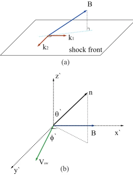
Figure 1 is a sketch that shows the basic points of the re-mote sensing local structure of the shock front. As shown in Fig. 1, a part of the incoming solar wind ions are reflected at the shock front to travel along the magnetic field line, which has a convection velocity (Vsw) towards the downstream of
bow shock. The velocity and intensity of those reflected ion beams (FABs) are affected by the geometry of shock front. The variation of FABs’ velocity may indicate the uneven shock surface. Thus, the local structure of bow shock can be estimated by using the geometry relationship between the observed FABs’ velocity, velocity of solar wind and mag-netic field.
The reflected FABs are recognized as a fraction of re-flected solar wind ions, which are accelerated by the mo-tional electric field at the bow shock. The velocity of FABs are well explained by the direct reflection model introduced by Sonnerup (1969), which is also called asµconserving re-flection by Schwartz et al. (1983) due to the conservation of ions’ magnetic momentsµm. In the direct reflection model, a
simple geometrical relationship between shock normal n, up-stream IMF B, incoming solar wind velocity Vsw and FABs
velocity Vb is defined. It is convenient to describe the
di-rect reflection model in the de Hoffman-Teller (HT) frame
(de Hoffman and Teller, 1950), which is a moving frame to cancel out the motional electric field at the bow shock. Ac-cordingly, the direct reflection model shows the conservation of kinetic energy of incoming and reflecting ions flow in the HT frame.
The following equation is the definition of the HT velocity:
VH T =
n×(Vsw×B)
B·n , (1)
which is equivalent to the following equation (Schwartz and Burgess, 1984):
Vb0
Vsw0
= cosθBn
cosθV n
cosθBV + s
Vb2 V2
sw
−sin2θBV
−1. (2)
Vb0 andVsw0 are velocities of FABs and solar wind in the
HT frame;VbandVsware velocities of FABs and solar wind
in the spacecraft frame, respectively. θBV is the acute angle
between B and Vsw.
The assumption of energy conservation of ion flow re-quires the left hand side of the Eq. (2) is equal to 1.
Vb0
Vsw0
=1 (3)
The each component of vector Eq. (1) can be written as one set of homogenous linear equations about shock normal n. Unfortunately, the rank of the coefficients matrix is 1, so that the n cannot be determined uniquely. Thus, the additional constraints of n are necessary to be introduced as follows:
1. n is always pointing to the upstream from the down-stream of bow shock;
2. n is first assumed in the Vsw–B plane; subsequently, we
allow n is out of the Vsw–B plane with some certain
angle as shown in Fig. 2b.
The B, Vband Vsw in Eq. (2) are all obtained by the
obser-vation. Thus, Eqs. (2), (3) and additional constraints can be used to calculate the n uniquely.
2.2 Motion of the average shock front
In order to determine the uneven shock surface, we need to trace the FABs to their origin at the shock front and then calculate shock normal vectors on the shock front. Tracing the FABs to the shock front requires the location and motion of the average shock front. Using timing analysis method (e.g. Russell et al., 1983; Harvey, 1998; Schwartz, 1998), the shock normal vectors and shock speeds are determined at in-bound or outin-bound shock crossing events. Based on the ve-locities of the shock front at crossing events, the motion of the average shock front (the black horizontal straight line in Fig. 1) between the two crossings is deduced. The shock ve-locity at the first crossing is as the initial veve-locity (vi) and the
n
B
x
S/C
Shock front Vb
Vsw
θBn
t0
[image:3.595.310.540.63.364.2]t1
Fig. 1. The black horizontal straight line is the average shock front and the vertical black arrow is the shock normal n; the black dashed curve is the possible shock structure and the light blue arrows are the local shock normal vectors (not to scale); The red arrow is the velocity of FABs; The blue dashed and solid lines are IMF at
dif-ferent time which is moving with Vsw; The beam is located at the
shock att0, while arriving at the location of SC3 att1; x is the
pro-jection of the FABs traveling path along the shock front.
(vf). If the viand vf are approximately along a straight line
(shown as a vertical dashed line in Fig. 1), the motion of the shock can be simplified to a 1-D motion (The details will be described in Sect. 3). After the shock normal vectors are lo-cated (i.e. the x in Fig. 1 is determined), we may describe the local structure of shock front, accordingly.
2.3 Use surface waves to describe the local structure Hybrid simulations are used to find the properties of the sur-face waves we are most likely seeing at those shock cross-ings. In a recent paper (Burgess and Scholer, 2007), authors pointed out that the gyrating ion population at the shock front is closely associated with the waves at the shock ramp. We used the results of this paper to obtain limits for the wave-length and amplitude for our model described below.
In our current model we introduce two surface waves, per-pendicular to each other, which are preestablished at the av-erage shock front (so called forward model), as shown in Fig. 2a. Those two surface waves are marked as k1and k2.
The wave k1is roughly along the projection of upstream IMF
B.
The goal of our numerical approach is using the direct reflection model and reproducing the observed bulk beams speed variations by introducing sinusoidal waves, which sim-ulates the local shock structure. In an iterative process wave-length and amplitude are updated to obtain the best fit to the observed time series of the FABs speeds.
B
k
2k
1shock front
x`
z`
y`
V
swB
φ
θ
n
`
`
(a)
(b)
Fig. 2. (a) 2-D plane surface waves are added to the shock front to reproduce the measured FABs; the projection of the B is set as a
referred direction; Plane waves k1and k2are perpendicular to each
other. (b) shows the correspondent coordinate system where the
shock normal vector n is out of the B–Vswplane.
3 Data
For this study observational data are provided by the Clus-ter spacecraft. We use the fluxgate magnetomeClus-ter (FGM) to obtain high time resolution (about 22 measurements per second) magnetic field data (Balogh et al., 2001); and the composition and distribution function analyzer (CODIF) to obtain the proton’s distribution function in velocity space. The solar wind bulk velocity is derived from hot ion analyzer (HIA) (R`eme et al., 2001). Both CODIF and HIA sensors are called CIS (Cluster Ion Spectrometry) instruments.
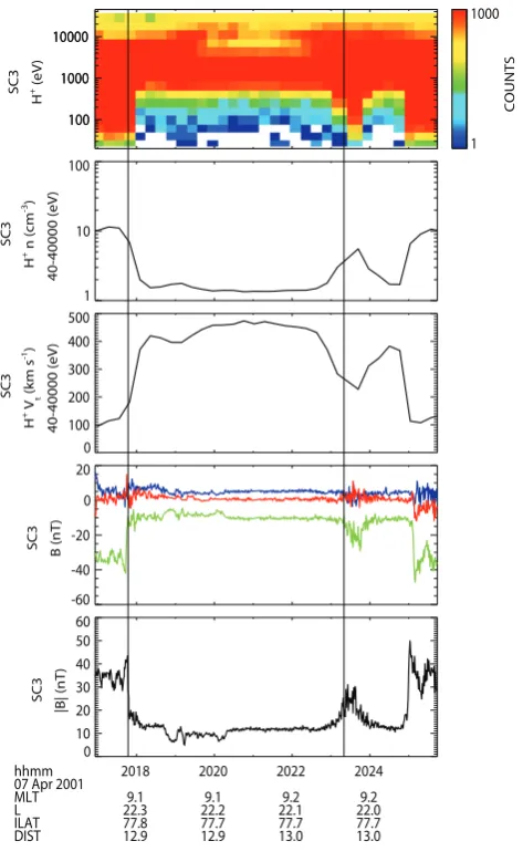
For the present study we identified the following shock crossing events: on 7 April 2001, 20:17:00–20:23:00 UTC, on 29 December 2003, 05:41:00–05:46:00 UTC, on 14 Jan-uary 2004, 08:12:00–08:15:00 UTC and on 3 April 2004, 20:51:00–21:06:00 UTC which will be discussed in detail. During these time periods, the separation of the Cluster spacecraft was between 400 and 1000 km.
[image:3.595.49.290.65.216.2]100 1000 10000
SC3
H
+ (eV)
100 1000 10000
1 1000
COUNTS
1 10 100
SC3
H
+ n (cm -3)
40-40000 (eV)
0 100 200 300 400 500
SC3
H
+ V
t
(km s
-1)
40-40000 (eV)
-60 -40 -20 0 20
SC3 B (nT)
2018 9.1 22.3 77.8 12.9
2020 9.1 22.2 77.7 12.9
2022 9.2 22.1 77.7 13.0
2024 9.2 22.0 77.7 13.0 0
10 20 30 40 50 60
[image:4.595.50.287.61.451.2]SC3
|B| (nT)
hhmm 07 Apr 2001 MLT L ILAT DIST
Fig. 3. The top panel is proton’s energy spectrum according to Clus-ter SC3 CODIF’s data. The remaining panels are number density of protons, bulk velocity of protons, B and magnitude of B . The two vertical lines mark the positions of shock crossing events.
bulk speeds, each component of the magnetic field and its magnitude as a function of time from spacecraft 3 (SC3). Vertical lines mark the outbound and the inbound crossings, respectively. Clearly, the sudden changes in the solar wind speeds, density, and magnetic field can be identified. Up-stream of the shock, in the solar wind, we observe a high energy populations at∼10 keV (the field-aligned ion beams as we will discuss later).
3.1 Average shock normal and shock speeds
In order to trace the FABs to the shock front, the location of the shock front is required. To determine the actual shock position we take advantage of Cluster as a multi-spacecraft mission and we perform a timing analysis between two con-secutive shock crossings. Using vi, vf, initial displacement,
si, and final displacement, sf, the displacement of shock
front can be simplified as a three-order polynomial function of time (Haaland et al., 2004), i.e.:
s(t )=a0+a1t+a2t2+a3t3, (4)
and then the velocity of shock front is:
v(t )=a1+2a2t+3a3t2. (5)
For our investigations we have chosen two adjacent shock crossings. Timing analysis method has been used to de-termine the shock normal of ni = (0.91, −0.12, 0.18) and
shock speed of vi=14 km s−1 at outbound crossing, left
side of Fig. 3; At inbound crossing, right side of Fig. 3, shock normal nf=(0.95, −0.18, 0.27) and shock speed of
vf=5 km s−1. The time span between the shock crossings is
of the order of 6 min. As one can see, the two shock nor-mal vectors niand nf are nearly the same, with difference of
about 5.5◦. Thus, we assume that, between the two crossing events, the shock front is moving with a non-constant accel-eration in one dimension. This allows us to determine the distance to the shock front by solving the equations of mo-tion.
3.2 Observation of field-aligned beams
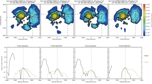
For this study a number of shock crossings have been inves-tigated. In the top panel of Fig. 3, a beam like feature can be identified in the energy spectrum at around 10 keV. The proton phase space distribution clearly shows that FABs are present. The best time resolution of CIS instrument is one spin period, i.e. 4 s. For our case study, distribution func-tions are accumulated for all 16 energy levels in the energy range from 10 to 40 keV, over 16 s. The top panel of Fig. 4 shows a time series of distribution functions in the velocity space; the bottom panel of Fig. 4 shows 1-D cuts through the center of the FABs, along theVpara(green line) andVperp
(black line) directions, respectively. In the figure, Vpara is
the velocity parallel to the IMF B whereas Vperp denotes
the component that is perpendicular to the magnetic field. The yellow pattern, withVpara=−450 km s−1 at the core, is
the solar wind distribution and the light blue pattern, with
Vpara=1200 km s−1 at the core, is FABs distribution, which
has inverse sign ofVparaand similarVperp while comparing
to the bulk velocity of the solar wind. The magnitude of the FABs velocity is given byVb=
q V2
para+Vperp2 . The beams can
Sat 3 CLUSTER CODIF H+ (Product 12) 07- 04- 2001/20:19:33->20:19:49
-2000 -1000 0 1000 2000
V Para (km/sec) -2000
-1000 0 1000 2000
V Perp (km/sec)
Cross Sections
-2000 -1000 0 1000 2000
Velocity (km/sec) 10-12
10-11
10-10
10-9
10-8
10-7
10-6
f (sec^3 / km^3 /cm^3)
Sat 3 CLUSTER CODIF H+ (Product 12) 07- 04- 2001/20:20:21->20:20:37
-1000 0 1000 2000
V Para (km/sec)
Cross Sections
-1000 0 1000 2000
Velocity (km/sec)
Sat 3 CLUSTER CODIF H+ (Product 12) 07- 04- 2001/20:20:53->20:21:09
-1000 0 1000 2000
V Para (km/sec)
Cross Sections
-1000 0 1000 2000
Velocity (km/sec)
Sat 3 CLUSTER CODIF H+ (Product 12) 07- 04- 2001/20:21:41->20:21:57
-1000 0 1000 2000
V Para (km/sec)
5.0•10-13
2.1•10-12
9.1•10-12
3.9•10-11
1.7•10-10
7.1•10-10
3.0•10-9
1.3•10-8
5.5•10-8
2.3•10-7
1.0•10-6
f (sec^3 / km^3 /cm^3)
Cross Sections
-1000 0 1000 2000
Velocity (km/sec)
V para
[image:5.595.47.546.63.338.2]V perp
Fig. 4. Proton’s distribution functions in the velocity space are shown in the spacecraft frame. The V-para axis is along direction of IMF measured by Cluster’s FGM instrument and the V-perp axis is a direction normal to IMF. From the left panel to right panel are distribution functions on 7 April 2001 at 20:19:33–20:19:49 UTC, 20:20:21–20:20:37 UTC, 20:20:53–20:21:05 UTC and 20:21:41–20:21:57 UTC. Top panel shows the 2-D distribution function, while the bottom panel shows a cut along the distributions function indicated by the dashed lines.
4 Results from our numerical study
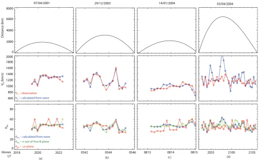
In this section we will now apply our numerical model which has been introduced in Sect. 2. As described above we will iteratively vary the wave number and the wave amplitude of the introduced plane waves which are supposed to mimic the local shock structure. For our case studies, the FABs veloc-ity and calculatedθBnare reproduced by superimposing 2-D
surface plane waves onto the average shock surface. In Fig. 5 we show four selected shock crossings at which Cluster SC1 or SC3 observes FABs. SC1 observes these beams on 3 April 2004 at 20:51:00–21:06:00 UTC, whereas SC3 observes other events on 7 April 2001 at 20:17:00–20:23:00 UTC, on 29 December 2003 at 05:41:00– 05:46:00 UTC and on 14 January 2004 at 08:12:00– 08:15:00 UTC. From top to bottom this figure shows the dis-tance of the spacecraft to the shock front determined by tim-ing analysis, the beams bulk speeds and the shock normal angles determined by the models. In the middle panels of Fig. 5a, b and c the observed velocities of FABs are well re-produced. The red lines show the observed FABs speeds; the blue lines represent the calculated FABs speeds. As one can see, the numerical models reproduce the observed beams’ bulk speeds very well. In the bottom panel we showθBn
determined by the various methods. The blue lines show the
θBn calculated with the preestablished local structure (sine
wave) according to the forward model; the green lines show the θBn calculated with Eqs. (2), (3) and constraint that n
is out of B–Vsw plane with the selected angle; the red lines
show theθBncalculated with the similar way as green lines
but n is within the B–Vsw plane. The green lines are
per-fectly matched with the blue lines. Due to the lack of match between blue and red lines, the n, B and Vswcoplanar model
cannot reproduce theθBn. Schwartz and Burgess (1984) also
mentioned that “the direction of n does not, in general, lie in the B–Vsw plane”. These results are obtained for the
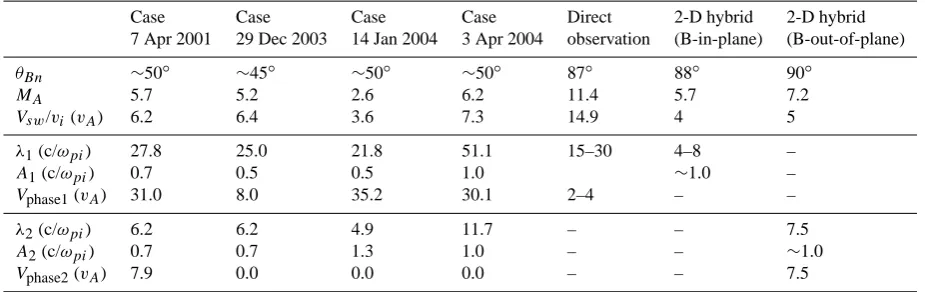
param-eters listed in Table 1 (first 3 rows).
The local structure may be approximately described by those 2-D surface plane waves. The surface plane wave by using subscript 1 (λ1,A1,Vphase1), is corresponding to the
B-in-plane-wave according to the 2-D hybrid simulation work (Burgess and Scholer, 2007); The surface plane wave by us-ing subscript 2 (λ2,A2,Vphase2), is corresponding to the
B-out-of-plane-wave. From Table 1, the B-in-plane-wave has long wavelength and small amplitude which is interpreted as an ultra-low frequency surface wave. The variation of FABs velocity is mainly affected by the B-out-of-plane-wave, wave
Distance (km)
600 800 1000 1200 1400 1600 1800 2000
Vb
(km/s)
2018 2020 2022 0
20 40 60 80
θBn
hhmm
07/04/2001
θBn -- calculated from wave
θBn -- n out of Vsw-B plane θBn -- co-plane Vb -- observation
Vb -- calculated from wave
0813 0814 0815 14/01/2004
0542 0544 0546 29/12/2003
2055 2100 2105 03/04/2004
(b) (c) (d)
UT
(a)
[image:6.595.45.551.61.376.2]0 2000 4000 6000 8000
Fig. 5. The top panels for the distance from the SC3 to the average shock front; the middle panels for the speed variations of the observed
FABs (red line) and the calculated FABs (blue line) according to the forward model; the bottom panels for theθBnand the blue line for the
forward model, the green line for the n out of B–Vswplane analytic method, the red line for the n, B and Vswcoplanar.
For the 7 April 2001 case, the angle of n out of the B–Vsw
plane is 15◦; For the 29 December 2003 case, the n is 20◦ out of the plane; For the 14 January 2004 case, the n is 30◦ out of the plane. The matched shock normal anglesθBn
indi-cate the shock normal vectors n are limited in a plane. This means that the 1-D surface wave (limited in our case studies) mainly controls the local structure of shock front. The differ-ent angles of n out of the plane indicate the contribution of surface wave k1to the local structure of the shock front.
In error analysis, the standard deviation of upstream Vsw
and high time resolution B can be obtained from the level 2 data of Cluster. Due to the middle panels of Fig. 5, the devi-ation between the observedVb and the calculated Vb from
wave is approximately recognized as the deviation of Vb.
Applying error propagation, we performed an error estimate (Bevington et al., 2003) forθBnthat is calculated from wave
(blue line) in the case study for 7 April 2001, in which we obtained4θBn=±3◦.
All three case studies (a, b and c) are in a relatively short time period, 3–5 min, and the 1-D surface wave k2 is the
major wave to describe the local structure perfectly. How-ever, for the case study for 3 April 2004 (Fig. 5d), the time
period is relatively longer, 10–15 min, and then the mono-frequency 1-D surface wave is no longer suitable to describe the local structure. The middle panel of Fig. 5d shows that the mono-frequency surface wave cannot reproduce the ob-served FABs speeds; the bottom panel of Fig. 5d also shows that the constraint (n out of plane with one certain angle) is not applicable, in this case study, to reproduce the θBn.
Table 1. Plasmas and wave parameters: comparison of 4 case studies 2-D surface plane waves, direct observation and 2-D hybrid simulation results.
Case Case Case Case Direct 2-D hybrid 2-D hybrid
7 Apr 2001 29 Dec 2003 14 Jan 2004 3 Apr 2004 observation (B-in-plane) (B-out-of-plane)
θBn ∼50◦ ∼45◦ ∼50◦ ∼50◦ 87◦ 88◦ 90◦
MA 5.7 5.2 2.6 6.2 11.4 5.7 7.2
Vsw/vi(vA) 6.2 6.4 3.6 7.3 14.9 4 5
λ1(c/ωpi) 27.8 25.0 21.8 51.1 15–30 4–8 –
A1(c/ωpi) 0.7 0.5 0.5 1.0 ∼1.0 –
Vphase1(vA) 31.0 8.0 35.2 30.1 2–4 – –
λ2(c/ωpi) 6.2 6.2 4.9 11.7 – – 7.5
A2(c/ωpi) 0.7 0.7 1.3 1.0 – – ∼1.0
Vphase2(vA) 7.9 0.0 0.0 0.0 – – 7.5
5 Discussion
From those case studies presented above we infer amplitudes, wavelengths and phase speeds of the local shock structure at the shock ramp on 7 April 2001, 29 December 2003 and 14 January 2004 (Table 1, last 6 rows). For the 7 April 2001 case, amplitudeA=50 km, wavelengthλ=440 km and
ω=8.0ωci. The wave parameters are normalized by
up-stream ion initial length (c/ωpi∼71 km) or Alfv´en velocity
(vA∼82 km s−1) as follows:λ=2π/k=6.2 c/ωpi,A=0.7 c/ωpi
andvphase=7.9vA. These plasma parameters are based on
average value of θBn=55◦ to 60◦, Alfv´en Mach number
MA=5.3 andVsw=530 km s−1.
In the 2-D hybrid simulation of Lowe and Burgess (2003), the surface waves propagating along the shock haveλ=4 to 8 c/ωpiwhenθBn=88◦,MA=5.7,βi=0.5 andVin=4vA(Vinis
the bulk velocity of incoming ions in the upstream, i.e. solar wind velocity).
In the most recent simulation of Burgess and Scholer (2007), they repeated the 2-D hybrid simulation with B in the simulation plane and obtained a wavelengthλ=6 c/ωpi,
MA=5.0 and βi=0.5 for the surface waves (ripples). They
also reported on simulations of the ripple structures with magnetic field orientations out-of-plane. The ripple wave-length is 7.5 c/ωpi(as obtained from Fig. 3. in Burgess and
Scholer, 2007) forMA=7.6 andβi=0.5. This wavelength is
longer than the one obtained from the simulation with B-in-plane (λ=2–5 c/ωpi,MA=7.1 andβi=0.5). From Table 1, our
results are close to the results of B-out-of-plane hybrid sim-ulation. One difference, however, should be noted that their 2-D hybrid simulation work has B in the simulation plane, i.e. propagating direction k of surface wave, shock normal n and B are co-planar. In our case study the wave vector k is not co-planar with B and n. The k is around 30◦biased from the direction of projection of upstream B instead. The reason for this biased angle is still an open question.
Recent observations of ripples on the quasi-perpendicular shock front by Moullard et al. (2006) have been interpreted
as traveling ripples within the thin shock layer with a phase speed of 2 to 4 timesvA(i.e. 80–160 km s−1) roughly along B, a wavelength of approximately 15 to 30 times c/ωpi, i.e.
1000–2000 km andMA=11.4 (shown Direct observation
col-umn of Table 1). Moullard et al. have noted the obvious dis-crepancy in the ripple wavelength and phase speed between their observations and the 2-D hybrid simulation results. Due to different plasma conditions in Moullard’s and our analysis, we cannot compare both observations directly. The differ-ences between the two observations indicate that there may be a variation in wavelength and phase speed for those sur-face waves in the quasi-perpendicular shock front depending on the plasma conditions.
Another problem on the analysis is the difference ofθBn
which is obtained by using different method. In Fig. 5, for example, 7 April 2001 case shows that theθBnis about 50◦,
which is somewhat lower than the averageθBnabout 55◦to
60◦given by the timing analysis method. This is due to the pitch angle scattering of FABs (Kucharek et al., 2004), in which the parallel component of Vbis decreasing while the
perpendicular component of Vb is increasing. If we use the
FABs peak pattern in the distribution function, the measured velocity of FABs would be lower than the theoretical veloc-ity of FABs (without considering scattering effect) predicted by the direct reflection model andθBn(determined by
tim-ing analysis method). Thus, underestimated FABs velocity might cause a lowerθBn.
In our analysis, the spatial resolution of the local shock structure is mainly limited by the time resolution of CODIF data (16 s in our case study). The accuracy in the studies of the shock surface structure using FABs also depends on shock motion, θBn, θV n, and the solar wind velocity. For
example, during 7 April 2001, 20:19:00–20:22:00 UTC, the shock normal angle of average shock frontθBn = 55◦ and
averaged in 16 s is originated from shock surface with a length of up to hundred kilometers. Because the wavelength of major 1-D surface plane wave is 440 km (7 April 2001 case) according to our analysis, the spatial resolution of our method is high enough to reveal the surface waves in the case study. However, if the averageθBnis close to 90◦, the
reso-lution would be dramatically lower. The resoreso-lution also de-creases as well as the shock speed inde-creases.
Our analysis requires high energy and angular resolution of FABs. The CODIF instrument has angular resolution of 11.5◦and global data interpolation is necessary to gain the direction of peak distribution of FABs. This is the another source of uncertainty.
According to the numerical simulations (e.g. Lemb`ege and Savoini, 1992; Hada et al., 2003; Scholer et al., 2003), shock self-reformation can lead to variation of the locations of the quasi-perpendicular shock. This process also causes vari-ation of the θBn and this in turn leads to the variation of
FABs’ velocity and intensity. In this study, we have used sinusoidal waves which are superposed on a planar shock to reproduce the velocity variation of FABs. Good agreement with observation has been achieved. In principal, the range of plasma parameters allows reformation, therefore we can-not exclude self-reformation. TheMA of the selected cases
is about 5 (see Table 1) andβi is 0.5 or higher. Shock
self-reformation is observed under the cases that have the higher
MAand lowerβi (less than 0.4) in the simulations (Lemb`ege
and Savoini, 1992). However in the later full particle sim-ulation by Hada et al. (2003), which has larger ion/electron mass ratio (∼84), shows that the self-reformation may oc-cur at relatively lowMA (2–5) and it disappears whenβi is
high. The average shock normal angles of the cases, 55◦– 60◦, are close to 62◦ which is the critical angle when self-reformation occurs (Lemb`ege and Savoini, 1992). However, due to the time resolution of the CIS instrument we would not be able to distinguish the effect of shock ripples and shock reformation. Similar discussion on CIS observation and self-reformation can be found in Meziane et al. (2007) and Lobzin et al. (2007). High resolution FGM data might provide more information on distinguishing shock ripples and reformation. However, we consider this as a subject of future investiga-tions.
6 Summary
In this paper we have introduced a new technique that al-lows us to remote sense the local structure of the quasi-perpendicular Earth’s bow shock. For this study we have assumed that the variations of the bulk velocity of the FABs are associated with local changes of the shock normal angle caused by surface waves or surface ripples. These assump-tions are based on the direct reflection model. The proposed model is an iterative numerical model that allows to intro-duce 2-D surface waves that simulate the local shock
struc-ture. Wavelength and wave amplitudes are variables which are determined by fitting the observed time variations of the FABs. We have introduced a basic approach in which we have limited the shock normal to lie in the plane of the in-coming solar wind and the interplanetary magnetic field. In a second approach we even allowed shock normals out of that plane.
The comparison of the obtained wavelength and ampli-tudes from this model with hybrid simulations showed very good agreement. The limitation of this approach for long time period cases might be solved by introducing multi-frequency and multi-dimension surface waves. It should be noted that the advantage of such approach is that the space-craft does not have to measure in the shock ramp to provide information of the local shock structure. Shock crossings are usually fast and data are limited. Furthermore, such an ap-proach is not limited to the Earth’s bow shock. It can be applied to any other stationary shock which is not so easily accessable such as the termination shock.
Acknowledgements. This work was supported by NASA under the
grant number NNG04GF23G.
Topical Editor R. Nakamura thanks D. Burgess and another anonymous referee for their help in evaluating this paper.
References
Asbridge, J. R., Bame, S. J., and Strong, I. B.: Outward flow of protons from the Earth’s bow shock, J. Geophys. Res. 73(12), 5777–5782, 1968.
Bale, S. D., Mozer, F. S., and Horbury, T. S.: Density-Transition Scale at Quasiperpendicular Collisionless Shocks, Phys. Rev. Lett., 91, 265004, doi:10.1103/PhysRevLett.91.265004, 2003. Bale, S. D., Balikhin, M. A., Horbury, T. S., Krasnoselskikh, V. V.,
Kucharek, H., M¨obius, E., Walker, S. N., Balogh, A., Burgess, D., Lemb`ege, B., Lucek, E. A., Scholer, M., Schwartz, S. J., and Thomsen, M. F.: Quasi-perpendicular Shock Structure and Processes, Space Sci. Rev., 118, 1–4, 161, doi:10.1007/s11214-005-3827-0, 2005.
Balogh, A., Carr, C. M., Acu˜na, M. H., Dunlop, M. W., Beek, T. J., Brown, P., Fornacon, H., Georgescu, E., Glassmeier, K.-H., Harris, J., Musmann, G., Oddy, T., and Schwingenschuh, K.: The Cluster Magnetic Field Investigation: overview of in-flight performance and initial results, Ann. Geophys., 19, 1207–1217, 2001, http://www.ann-geophys.net/19/1207/2001/.
Bevington, P., Robinson, D., Bruflodt, D., and Cotkin, S. (Eds.): Data Reduction and Error Analysis, McGraw-Hill, Kent A. Pe-terson, USA, 2003.
Burgess, D. and Scholer, M.: Shock front instability associated with reflected ions at the perpendicular shock, Phys. Plasmas, 14, 012108, doi:10.1063/1.2435317, 2007.
Gosling, J. T., Asbridge, J. R., Bame, S. J., Paschmann, G., and Sckopke, N.: Observations of two distinct populations of bow shock ions in the upstream solar wind, Geophys. Res. Lett., 5, 957–960, 1978.
Haaland, S. E., Sonnerup, B. U. ¨O., Dunlop, M. W., Balogh, A., Georgescu, E., Hasegawa, H., Klecker, B., Paschmann, G., Puhl-Quinn, P., R`eme, H., Vaith, H., and Vaivads, A.: Four-spacecraft determination of magnetopause orientation, motion and thick-ness: comparison with results from single-spacecraft methods, Ann. Geophys., 22, 1347–1365, 2004,
http://www.ann-geophys.net/22/1347/2004/.
Hada, T., Oonishi, M., Lemb`ege, B., and Savoini, P.: Shock front nonstationarity of supercritical perpendicular shocks, J. Geo-phys. Res., 108(A6), 1233, doi:10.1029/2002JA009339, 2003.
Harvey, C. C.: Spatial gradients and the volumetric tensor,
in: Multi-Spacecraft Analysis, Chap. 12, ISSI, edited by:
Paschmann, G. and Daly, P., 307–348, 1998.
Horbury, T. S., Cargill, P. J., Lucek, E. A., Eastwood, J., Balogh, A., Dunlop, M. W., Fornacon, K.-H., and Georgescu, E.: Four space-craft measurements of the quasiperpendicular terrestrial bow shock: Orientation and motion, J. Geophys. Res., 107, 1208– 1219, doi:10.1029/2001JA000273, 2002.
Kucharek, H., M¨obius, E., Scholer, M., Mouikis, C., Kistler, L. M., Horbury, T., Balogh, A., R`eme, H., and Bosqued, J. M.: On the origin of field-aligned beams at the quasi-perpendicular bow shock: multi-spacecraft observations by Cluster, Ann. Geophys., 22, 2301–2308, 2004,
http://www.ann-geophys.net/22/2301/2004/.
Lin, R. P., Meng, C. I., and Anderson, K. A.: 30–100 keV protons upstream from the Earth bow shock, J. Geophys. Res., 79, 489– 498, 1974.
Lemb`ege, B. and Savoini, P.: Nonstationarity of a two-dimensional quasiperpendicular supercritical collisionless shock by self-reformation. Phys. Fluids, B, 4, 3533–3548, 1992.
Lobzin, V. V., Krasnoselskikh, V. V., Bosqued, J.-M., Pinc¸on, J.-M., and Schwartz, S. J.: Nonstationarity and reformation of high-Mach-number quasiperpendicular shocks: Cluster observations, Geophys. Res. Lett., 34, L05107, doi:10.1029/2006GL029095, 2007.
Lowe, R. E. and Burgess, D.: The properties and causes of rippling in quasi-perpendicular collisionless shock fronts, Ann. Geophys., 21, 671–679, 2003, http://www.ann-geophys.net/21/671/2003/. Meziane, K., Wilber, M., Hamza, A. M., Mazelle, C., and Parks,
G. K.: Evidence for a high-energy tail associated with fore-shock field-aligned beams, J. Geophys. Res., 112, A01101, doi:10.1029/2006JA011751, 2007.
Moullard, O., Burgess, D., Horbury, T. S., and Lucek, E.
A.: Ripples observed on the surface of the Earth’s
quasi-perpendicular bow shock, J. Geophys. Res., 111, A09113, doi:10.1029/2005JA011594, 2006.
M¨obius, E., Kucharek, H., Mouikis, C., Georgescu, E., Kistler, L. M., Popecki, M. A., Scholer, M., Bosqued, J. M., R`eme, H., Carlson, C. W., Klecker, B., Korth, A., Parks, G. K., Sauvaud, J. C., Balsiger, H., Bavassano-Cattaneo, M.-B., Dandouras, I., DiLellis, A. M., Eliasson, L., Formisano, V., Horbury, T., Lennartsson, W., Lundin, R., McCarthy, M., McFadden, J. P., and Paschmann, G.: Observations of the spatial and temporal structure of field-aligned beam and gyrating ring distributions at the quasi-perpendicular bow shock with Cluster CIS, Ann. Geo-phys., 19, 1411–1420, 2001,
http://www.ann-geophys.net/19/1411/2001/.
Paschmann, G., Sckopke, N., Asbridge, J. R., Bame, S. J., and Gosling, J. T.: Energization of solar wind ions by reflection from the Earth’s bow shock, J. Geophys. Res., 85, 4689–4693, 1980. R`eme, H., Aoustin, C., Bosqued, J. M., et al.: First multispacecraft
ion measurements in and near the Earth’s magnetosphere with the identical Cluster ion spectrometry (CIS) experiment, Ann. Geophys., 19, 1303–1354, 2001,
http://www.ann-geophys.net/19/1303/2001/.
Russell, C. T., Mellott, M. M., Smith, E. J., and King, J. H.: Multiple spacecraft observations of interplanetary shocks Four spacecraft determination of shock normals, J. Geophys. Res., 88, 4739–4748, 1983.
Scholer, M., Shinohara, I., and Matsukiyo, S.: Quasi-perpendicular shocks: Length scale of the cross-shock potential, shock ref-ormation, and implication for shock surfing, J. Geophys. Res., 108(A1), 1014, doi:10.1029/2002JA009515, 2003.
Schwartz, S. J., Thomsen, M. F., and Gosling, J. T.: Ions upstream of the Earth’s bow shock – A theoretical comparison of alterna-tive source populations, J. Geophys. Res., 88, 2039–2047, 1983. Schwartz, S. J. and Burgess, D.: On the theoretical/observational comparison of field-aligned ion beams in the Earth’s foreshock, J. Geophys. Res., 89, 2381–2384, 1984.
Schwartz, S. J.: Shock and discontinuity normals, mach numbers, and related parameters, in: Multi-Spacecraft Analysis, Chap. 10, ISSI, edited by: Paschmann, G. and Daly, P., 249–270, 1998.
Sonnerup, B. U. ¨O.: Acceleration of particles reflected at a shock