Volume 6, Number 2, pp. 45–57. http://www.scpe.org c 2005 SWPS
ON THE EXTENSION AND APPLICABILITY OF THE P-GRAPH MODELING PARADIGM TO SYSTEM-LEVEL DIAGNOSTIC PROBLEMS
BAL ´AZS POLG ´AR† , ENDRE SEL´ENYI† , ANDTAM ´AS BARTHA‡
Abstract.
This paper presents a novel approach that formulates different types of diagnostic problems similarly. The main idea is the reformulation of the diagnostic procedures as P-graph models. In this way the same paradigm can be applied to model different aspects of a complex problem. The idea is illustrated by solving the probabilistic diagnosis problem in multiprocessor systems and by extending it with some additional properties. Thus, potential link errors and intermittent faults are taken into consideration and the comparator based diagnostics is formulated including potential comparator errors.
Key words. multiprocessor systems, fault diagnosis, maximum likelihood diagnostics, modeling with P-graphs
1. Introduction. Diagnostics is one of the major tools for assuring the reliability of complex systems in information technology. In such systems the test process is often implemented on system level: the “intelligent” components of the system test their local environment and each other. The test results are collected, and based on this information the good or faulty state of each component is determined. This classification procedure is known asdiagnostic process.
The early approaches that solve the diagnostic problem employed oversimplified binary fault models, could only describe homogeneous systems, and assumed the faults to be permanent. Since these conditions proved to be impractical, lately much effort has been put into extending the limitations of traditional models [1]. However, the presented solutions mostly concentrated on a single aspect of the problem.
In this paper we present a novel modeling approach based on P-graphs that can integrate these extensions in one framework, while maintaining a good diagnostic performance. With this model, we formulate diagnosis as an optimization problem and apply the idea to the well-known multiprocessor testing problem. Furthermore, we have not only integrated existing solution methods, but proceeding from a more general base we have extended the set of solvable problems with new ones.
The paper is structured as follows. First an overview is given about the traditional aspects of system-level diagnosis [2, 3, 4] and the generalized test invalidation model used in our approach. Afterwards, the diagnostic problem of a multiprocessor system is formulated with the use of P-graphs [5]. In the fourth section two supplements are presented which can accelerate the solution method. Both use additional a priori information. The first one adds unit failure probabilities to the model, the second utilizes special knowledge about the structure of the system. Then an important aspect, the extensibility of the model is demonstrated via some examples. The generation and the solution method of a P-graph model and the acceleration techniques are clarified on a small example and simulation results are presented. Finally, we conclude and sketch the direction of future work.
2. System-Level Diagnosis. System-level diagnosis considers thereplaceable units of a system, and does not deal with the exact location of faults within these units. Asystem consists of an interconnected network of independent but cooperatingunits (typically processors). The fault state of each unit is eithergood when it behaves as specified, or faulty, otherwise. The fault pattern is the collection of the fault states of all units in the system. A unit may test theneighboring units connected with it via direct links. The network of the units testing each other determines thetest topology. The outcome of a test can be eitherpassed orfailed (denoted by 0/1 or G/F); this result is consideredvalid if it corresponds to the actual physical state of the tested unit.
The collection of the results of every completed test is called the syndrome. The test topology and the syndrome are represented graphically by the test graph. The vertices of a test graph denote the units of the system, while the directed arcs represent the tests originated at thetester and directed towards thetested unit (UUT). The result of a test is shown as the label of the corresponding arc. Label 0 represents the passed test result, while label 1 represents the failed one. See Figure 2.1 for an example test graph with three units.
†Dept. of Measurement and Inf. Systems, Budapest Univ. of Technology and Economics, Magyar Tud´osok krt. 2, Budapest,
Hungary, H-1117, ([email protected],[email protected]).
‡Computer and Automation Research Institute, Hungarian Academy of Sciences, Kende u. 13–17, Budapest, Hungary, H-1111,
Fig. 2.1.Example test graph (test topology with syndrome)
2.1. Traditional Approaches. Traditional diagnostic algorithms assume that (i) faults are permanent,
(ii) states of units are binary (good, faulty), (iii) the test results of good units are always valid,
(iv) the test results of faulty units can also be invalid. The behavior of faulty tester units is expressed in the form oftest invalidation models.
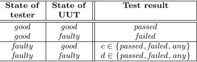
Fig. 2.2 shows the fault model of a single test and Table 2.1 covers the possible test invalidation models, where the selection ofcanddvalues determines a specific model. The most widely used example is the so-called PMC (Preparata, Metze, Chien) test invalidation model, (c=any, d=any) which considers the test result of a faulty tester to be independent of the state of the tested unit. According to another well-known test invalidation model, the BGM (Barsi, Grandoni, Maestrini) model (c = any, d = faulty) a faulty tester will always detect the failure of the tested unit, because it is assumed that the probability of two units failing the same way is negligible.
Fig. 2.2.Fault model of a single test
Table 2.1
Traditional test invalidation models
State of State of Test result tester UUT
good good passed
good faulty failed
faulty good c∈ {passed,failed,any}
faulty faulty d∈ {passed,failed,any}
The purpose of system-level diagnostic algorithms is to determine the fault state of each unit from the syndrome. The difficulty comes from the possibility that a fault in the tester processor invalidates the test result. As a consequence, multiple “candidate” diagnoses can be compatible with the syndrome. To provide a complete diagnosis and to select from the candidate diagnoses, the so-calleddeterministic algorithms use extra information in addition to the syndrome, such as assumptions on the size of the fault pattern or on the testing topology.
Alternatively,probabilistic algorithms try to determine the most probable diagnosis assuming that a unit is more likely good than faulty [6]. Frequently, this maximum likelihood strategy can be expressed simply as “many faults occur less frequently than a few faults.” Thus, the aim of diagnostics is to determine the minimal set of faulty elements of the system that is consistent with the syndrome.
Probabilitiespc0, pc1, pd0 and pd1 express the distortion of the test results by a faulty tester. Moreover, the generalized model is able to encompassfalse alarms (a good tester finds a good unit to be faulty) by setting probabilitypa1 to nonzero, however, it is not a typical situation.
Table 2.2
Generalized test model
State of State of Probability of test result
tester UUT 0 1
good good pa0 pa1
good faulty pb0 pb1
faulty good pc0 pc1
faulty faulty pd0 pd1
Of course, the generalized test invalidation model covers the traditional models. Setting the probabilities as pa0 = pb1 = 1, pc0 = pc1 = pd0 = pd1 = 0.5, and pa1 = pb0 = 0, the generalized model will have the characteristics of the PMC model, while the configuration pa0 = pb1 = pd1 = 1, pc0 = pc1 = 0.5 and
pa1=pb0=pd0= 0 will make it behave like the BGM model. Analogically, every traditional test invalidation model can be mapped as a special case to our model.
3. Diagnosis Based on P-Graphs. The name ’P-graph’ originates from the name ’Process-graph’ from the field of Process Network Synthesis problems (PNS problem for short) in chemical engineering. In connection with this field the mathematical background of the solution methods of PNS problems have been well elaborated, see [9, 10, 11].
3.1. Definition of the P-Graph Model of the Diagnostic System. A P-graph is a directed bipartite graph. Its vertices are partitioned into two sets, with no two vertices of the same set being adjacent. In our interpretation one of the sets contains hypotheses (assumptions or information about the state of units and the possible test results), the otherone containslogical relations between the hypotheses. Hypotheses are represented by solid dots and logical relations by short horizontal lines. The edges of the graph point from the premisses1
’through’ the logical relation to theconsequences2 .
The set of premisses contains all states of each unit (e.g., ’unit A is good’, ’unit A is faulty’, ’unit B is good’, denoted byAg, Af, Bg), and the set of consequences contains the test results (e.g. ’unit A finds unit
B to be good’, ’unit B finds unit C to be faulty’, denoted by ABG, BCF). Logical relations determine the
possible premisses of each possible test result. This means there are 8 logical relations for each test according to the 8 possible combinations of the state of tester, the state of the tested unit and the possible test results. Probabilities in Table 2.2 are assigned to relations expressing the uncertainty of the consequences. The P-graph model of a single-test fault model introduced on Fig. 2.2 can be seen on Fig. 3.1.
Fig. 3.1. P-graph model of a single test (vertices with same label represent a single vertex; multiple instances are only for better arrangement)
Asolution structureis defined as a subgraph of the original P-graph, which deduces the consequences back to a subset of premisses.
Constraints can be defined in the model in order to assure that in a solution structure a unit should have one and only one state. Formally, for each hypothesis h the function ǫ(h) determines the set of hypotheses which are excluded byh. A P-graph isconsistent if all constraints are satisfied.
The probability of the syndrome (PS) is the product of probabilities of relations in a solution structure.
This is the probability of occurrence of the consequences under the conditions of the given subset of system premisses, that is the probability of occurrence of the syndrome under the condition of a given fault pattern.
1
premiss: preliminary condition
2
During the solution process more consistent solution structures can exist having different subsets of premisses and having differentPS values. The object is to find the solution structure containing the subset of premisses
that implies the known consequences with maximum likelihood. This is an optimization task.
In principle, this task can be solved by general mathematical programming methods like mixed integer non-linear programming (MINLP), however, they are unnecessary complex. Friedler et al. [9, 10, 11] developed a new framework for solving PNS problems effectively by exploiting the special structure of the problem and the corresponding mathematical model.
3.2. Steps of the Solution Algorithm.
1. The maximal P-graph structure is generated. It contains only the relevant hypotheses and the relevant logical relations, but constraints are not yet satisfied. It contains all possible fault patterns being consistent with the given syndrome.
2. Every combinatorially feasible solution structure is obtained. These are the structures that satisfy the constraints and draw the consequences (i.e., the syndrome) back to a subset of the premisses. Each of these subsets determines a possible fault pattern.
3. For each combinatorially feasible solution structure the probability of syndrome is calculated. This is the conditional probability of the syndrome under the condition of a particular fault pattern.
4. The structure having the highest probability is selected; this solution structure contains the maximum-likelihood diagnosis.
Steps 2–4 can be completed either by a general solver for linear programming (since the generated maximal structure is a special flat P-graph), or with an adapted SSG algorithm [9]. Since the complexity of the generation of every combinatorially feasible solution structure in step 2 is exponential, the use of some kind of branch and bound technique can be employed to accelerate the solution method.
In a branch and bound algorithm a search tree is built. It branches as possible exclusive premisses are fixed for consequences. After a consistent solution is found, all those branches are bounded, which cannot have better PS value. The algorithm proceeds until all branches are either containing a solution structure or are bounded.
The algorithm can be more efficient if the first solution structure have been found quickly and it is near to the optimal one, because in this case bigger branches can be bounded.
4. Supplements to the Model. The base model described in the previous section can be supplemented or altered in order to increase the efficiency of the solution algorithm. In this section two enhancement methods are presented.
4.1. Probabilities of Unit Failures. Embedding more a priori information into the model does not necessarily increase the diagnostic accuracy, but it can speed up the solution algorithm. This is the case if unit failure probabilities are taken into account.
Let’s definepAg andpAf = 1−pAg as theprobability of the good and thefaulty state of unit A. Similarly,
probabilities for the states of other units are defined. If the system is homogeneous, the values are the same for each unit.
In the model these values are assigned to the vertices representing the corresponding state information of the unit (Fig. 4.1). It is similar, as probabilities were assigned to logical relations. Now the probability of the syndrome (PS) is defined as the product of probabilities of relations and premisses being in the solution
structure.
Fig. 4.1.P-graph model of a single test containing the probabilities of the states
This addition results in a bigger difference between the PS values of the more and the less probable fault
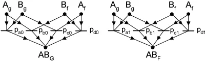
4.2. Mutual Tests. For special structures the model can be simplified or altered in order to increase the efficiency of the solution algorithm utilizing the extra information known about the system. An example for it is the case of mutual tests.
Tests t1 and t2 are mutual, if the tester in t1 is the tested unit in t2 and the tested unit in t1 is the tester in t2. Because the sets of possible premisses of the results of these tests are the same, the two tests can be handled together. Let’s substitute the two tests with one mutual test having four possible test results (GG,GF,FG,FF)(Fig. 4.2). The test invalidation model is modified according to Table 4.1.
Fig. 4.2.Fault model of a mutual test
Table 4.1
Probabilities of test result pairs depending on the states of units
State of State of Probability of test result pair A B ABGG ABGF ABF G ABF F good good pA0 pA1 pA2 pA3 good faulty pB0 pB1 pB2 pB3 faulty good pC0 pC1 pC2 pC3 faulty faulty pD0 pD1 pD2 pD3
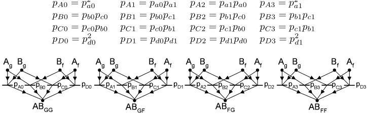
In the initial P-graph model the 2x2x4 logical relations (two pieces from the P-graph on Fig. 3.1) are replaced with 4x4 relations (Fig. 4.3). Although the size of the initial model is unchanged, after step 1 in solution algorithm the maximal structure contains only 4 relations instead of 2x4, because information is in a compact form in this model.
Of course, probabilities in Table 4.1 can be derived from the previous ones being in Table 2.2: pA0=p2a0 pA1=pa0pa1 pA2=pa1pa0 pA3=p2a1
pB0=pb0pc0 pB1=pb0pc1 pB2=pb1pc0 pB3=pb1pc1
pC0=pc0pb0 pC1=pc0pb1 pC2=pc1pb0 pC3=pc1pb1
pD0=p2d0 pD1=pd0pd1 pD2=pd1pd0 pD3=p2d1
Fig. 4.3.P-graph model of a mutual test
5. Extensions of the Model. The main contribution of this novel modeling approach is its generality. With its use several aspects of system-level diagnosis can be handled in the same framework. Furthermore, it became possible to formulate new aspects of diagnosis. Thus, it is possible to model and diagnose for instance the following cases:
Systems with heterogeneous elements. There are systems like thesupercomputer APEMille [12] which are built up from processing elements having different complexity and different behavior. These differences appear as the differences between the test invalidation models of the components. In the model it can be handled easily. Each element can have its own test invalidation model and the probability for the result of a test is taken from the invalidation model of the tester.
results anddead if it doesn’t operate or doesn’t communicate. This also implies that the result of a test can have more than two values as well.
The model of a system having mutual tests is an example for systems having multiple test results. To take multiple fault states into account, rows should be added to the test invalidation table according to the possible combinations of the states of the tester and tested unit. This will result in more logical relations in the P-graph.
Intermittent faults. These are permanent faults that become activated only in special circumstances. Because these circumstances are usually independent from the testing process, these type of faults are diagnosed for instance on the basis of multiple syndromes as in themethod of Lee and Shin [14].
Systems with potential link errors. The base model assumes that links between processors are working always properly. Conversely, the probability of the error of a link is not negligible in such systems where processors are connected to each other through routers as in the above mentionedParsytec GCel machine.
Systems based on the comparator model. The comparator based diagnostic model of multiprocessor sys-tems [15] is an alternative to the tester–tested unit model introduced by Preparata et al. In this model both units perform the same test and a comparator compares the bit-sequence of the outputs. In this case the syndrome consists of the results of the comparators, namely the information that’the two units differ’ or’the two units operate similarly’. Of course, this model can be applied only for homogeneous systems.
An example for the comparator based model is the previously mentioned commercially available APEMille supercomputer [12] which was developed in collaboration by IEI-CNR of Rome and Pisa, and the DESY Zeuthen in Germany.
A further possible application field of this model is the wafer scale diagnosis [15, 16]. The idea is to connect individual processors on the wafer in order to form a multiprocessor system just for the time of the diagnostic phase of the production. The advantage of it is that in this case processors can be tested on working speed—and not only on reduced speed—before packaging and the more faulty processors identified before packaging results in less cost.
The models of the last three items in the list are presented in details in the next subsections.
5.1. Modeling Intermittent Faults. Although handling of intermittent faults is one of the difficult to manage diagnostic problems, a possible solution is the use of multiple syndromes, as mentioned above. In this approach two or more testing rounds are performed in a row, and the possible differences between the subsequent syndromes are used to detect intermittent faults.
The adaptation of the diagnostic P-graph model to this approach is similar to the model of mutual tests. Considering the case of double syndromes the fault model, the test invalidation model and the P-graph model correspond to the appropriate models of mutual tests on Fig. 4.2, 4.3 and in Table 4.1 having differences in the testing method (Fig. 5.1) and in the derivation method of probability parameters.
Fig. 5.1.Fault model of a single test in case of double syndromes
pA0=p2a0 pA1=pa0pa1 pA2=pa1pa0 pA3=p2a1
pB0=p2b0 pB1=pb0pb1 pB2=pb1pb0 pB3=p2b1
pC0=p2c0 pC1=pc0pc1 pC2=pc1pc0 pC3=p2c1
pD0=p2d0 pD1=pd0pd1 pD2=pd1pd0 pD3=p2d1
In the general case n test rounds are performed in a row. Thus, 2n result combinations are in the fault
model and each containsnsingle test result. Consider the case when a result combination containsnG passed
and nF = n−nG failed test results. In this case the corresponding column in the test invalidation model
contains the derived probabilitiespnGa0 ·p
nF a1,p
nG b0 ·p
nF b1,p
nG c0 ·p
nF c1 ,p
nG d0 ·p
nF d1.
known about the system is increased, it is represented in a compact form in the probabilities while the size of the syndrome remains unchanged.
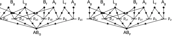
5.2. Modeling Systems with Potential Link Errors. The fault model of a single test shown on Fig. 2.2 is extended with theLink component (L) according to Fig. 5.2. For eachABtest a separate linkLAB
is assumed, which has either good or faulty state (denoted byLABg,LABf).
Fig. 5.2. Fault model of a single test with potential link error
The state of the link influences the test result, therefore the test invalidation table is modified according to Table 5.1. The probabilities are the same as in Table 2.2 if LAB is good, but additional parameters are
introduced if it is faulty.
Table 5.1
Probabilities of test results when considering the state of the link
State of State of State of Probability of test result
L A B ABG ABF
good good good pa0 pa1
good good faulty pb0 pb1
good faulty good pc0 pc1
good faulty faulty pd0 pd1
faulty good x pe0 pe1
faulty faulty x pf0 pf1
If a link failure means no communication between the two units, thenpe0= 0 (and thus,pe1= 1), because a good tester doesn’t produce thegood test result if it cannot reach the tested unit. But if a link failure means that noise is added to the signal during transmission through the link, then these additional probabilities can have arbitrary values according to the characteristics of the noise.
Fig. 5.3 shows the corresponding modified P-graph.
Fig. 5.3.P-graph model of a single test with potential link error
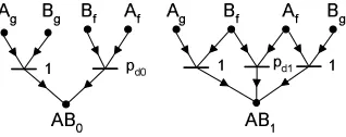
5.3. Modeling Comparator-Based Diagnostics. As mentioned above, in the comparison model pairs of units perform the same test and the outcomes are compared. The test result is 0 if they agree, and 1 otherwise (Fig. 5.4).
!
" #
" # $
Fig. 5.4.Fault model of a comparator based test
Table 5.2
Traditional test invalidation model of comparator based diagnostic models
Test result State of State of Malek’s model of
A B model Chwa & Hakimi
good good 0 0
good faulty 1 1
faulty good 1 1
faulty faulty 1 x
To be able to handle these models together, parameters are introduced in the test invalidation model for those state combinations, where test outcomes are not exactly determined. This is the case only if both units are faulty (Table 5.3). Parameters represent the probabilities of the 0/1 test outcomes. The application of probabilities means not only the unified handling of traditional models, but it allows to create a more realistic description of the behavior of the system.
Table 5.3
Generalized test invalidation model of comparator based diagnostic systems
State of State of Probability of test result
A B AB0 AB1
good good 1 0
good faulty 0 1
faulty good 0 1
faulty faulty pd0 pd1
As it can be seen in Table 5.3, this model arise as a special case of the generalized test invalidation model of the tester–tested unit approach. Hence, the corresponding P-graph appear to be the subgraph of that (the relations with 0 probability are eliminated). Fig. 5.5 shows the P-graph model of a single comparison test.
Fig. 5.5.P-graph model of a single comparator test
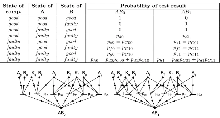
5.3.2. Model with Comparator Errors. The simple model can be extended in order to take into account the potential errors of the comparators. For simplicity, states of the comparators are assumed to be binary (good or faulty), see Fig. 5.6. According to the new component, the generalized test invalidation table is doubled and probabilities are assigned to both test results for all state combinations (Table 5.4).
Fig. 5.6. Fault model of a comparator based test with potential link error
Following the conversion rule of the invalidation table of a test into a P-graph model, the premisses of the relations are the state combinations, the consequences are the possible test results and the occurring probabilities in the table are assigned to the relations (Fig. 5.7).
The difficulty in creating the model is the determination of the conditional probabilities (for instance the probability of the 0 test result, if both units and the comparator are faulty). It is easier to examine the behavior of the comparator in itself and to derive the searched probabilities from it. Therefore thepC00,pC01,pC10,pC11 parameters are introduced, wherepCxy is the probability that a faulty comparator alters the result fromxtoy.
Table 5.4
Probabilities of test results in comparator based diagnostic model considering comparator errors
State of State of State of Probability of test result
comp. A B AB0 AB1
good good good 1 0
good good faulty 0 1
good faulty good 0 1
good faulty faulty pd0 pd1
faulty good good pe0=pC00 pe1=pC01 faulty good faulty pf0=pC10 pf1=pC11 faulty faulty good pg0=pC10 pg1=pC11 faulty faulty faulty ph0=pd0pC00+pd1pC10 ph1=pd0pC01+pd1pC11
Fig. 5.7. P-graph model of a single comparator test with potential comparator error
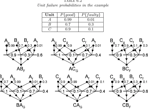
6. Example. Consider the test graph and syndrome given on Fig. 2.1 and the test invalidation model given in Table 6.1. Using the base modeling method the initial P-graph contains 6x7 logical relations where probabilities are assigned only to relations. After step 1 in the solution algorithm, the relevant structure contains the half of it, 3x4+3x3 pieces (see Fig. 6.1 without probabilities assigned to state information).
Table 6.1
Test invalidation model of the example
State of State of Probability of test result
tester UUT 0 1
good good 1 0
good faulty 0.1 0.9
faulty good 0.7 0.3
faulty faulty 0.4 0.6
During steps 2-4 at most eight solution structure can be generated because of the constraints. Each of it contains six logical relations. The eight structures correspond to the 23
possible fault patterns of the three units. That fault pattern is selected finally which produces the syndrome with the highest probability.
If the unit failure probabilities are known (Table 6.2), they can be assigned to the corresponding state information (Fig. 6.1). The ’only’ difference to the previously described solution is that the PS values of
subgraphs are different, but this is an important one. Actually it means that the difference between the conditional probabilities of the syndrome for different fault patterns is significantly larger. This results that the solution found at first is closer to the optimum and bigger branches can be bounded.
It can be observed in the first two rows of Table 6.3. The first five columns contain thePS values of the
five fault pattern which is consistent with the syndrome (the biggest value is boldfaced and the second biggest is in italic). The search tree contains 34 nodes if all five solution structure is determined. The sixth column contains the number of nodes which was accessed during the search. It decreased from 17 to 10 when unit failure probabilities were added to the model. The third and fourth rows contain these values for the case when the result of thetest BAwas changed fromBAGtoBAF. In this case the difference is more significant between
the two approaches.
Table 6.2
Unit failure probabilities in the example
Unit P{good} P{f aulty}
A 0.99 0.01
B 0.7 0.3
C 0.9 0.1
Fig. 6.1.Maximal P-graph structure of the base model of the example
Table 6.3
Fault patterns being consistent with syndrome; conditional probabilities of it for base/mutual model with and without unit failure probabilities (FP) and withBAG/BAF test result; size of the entire search tree (S) and the number of accessed nodes (n)
Ag Cg Ag Bg Cg base mutual
Bf Bf Cf Af Cf Af Bf AfBfCf (n/S) (n/S) BAG/ no FP 0.170 0.016 0.001 0.005 0.014 17/34 9/16
ABF G FP 0.045 5∗10−4 9∗10−7 1∗10−5 4∗10−6 10/34 7/16 BAF / no FP 0.073 0.007 0.011 0.007 0.021 25/34 11/16
ABF F FP 0.019 2∗10−4 8∗10−6 2∗10−5 6∗10−6 10/34 7/16
Fig. 6.2.Test graph of the example containing mutual tests
!"!# !" $ !"!#
%&
% %
!"$' !"() !"!'
% &&
% %
!"(# !"'$ !"(#
Fig. 6.3.Maximal P-graph structure of the mutual model of the example
The simulations were performed in a two-dimensional toroidal mesh topology, where each unit is tested by its four neighbors and each unit behaved according to the PMC test invalidation model. Statistical values were calculated on the basis of 100 diagnostic rounds. In every round the fault pattern was generated by setting each processor to be faulty with a given probability, independently from others.
average num ber of m isdiagnosed good processors relative to system size [%]
0 0.2 0.4 0.6 0.8 1 1.2 1.4
10 20 30 40 50 60 70 80 90 100
16 36 64 100
rate of rounds containing m isdiagnosed good processors [%]
0 20 40 60 80 100
10 20 30 40 50 60 70 80 90 100
16 36 64 100
average num ber of m isdiagnosed faulty processors relative to system
size [%] 0 1 2 3 4 5 6 7 8
10 20 30 40 50 60 70 80 90 100
rate of rounds containing m isdiagnosed faulty processors [%]
0 20 40 60 80 100
10 20 30 40 50 60 70 80 90 100
Fig. 7.1.Simulation results depending on unit failure probability
Accuracy of the solution algorithm: measurements were performed with system sizes of 4×4, 6×6, 8×8, 10×10 units, and the failure probability of units varied from 10% to 100% in 10% steps. On the diagrams in Figure 7.1 it can be observed that the algorithm has a very good diagnostic accuracy. Even if half of the units were faulty, good units were almost always diagnosed correctly. It is crucial in wafer scale testing because it means that none of good units are thrown away before packaging. Taking still the case when half of the units were faulty the rate of rounds containing misdiagnosed faulty units did not exceed 15%, and the rate of misdiagnosed units relative to the system size was under 1%.
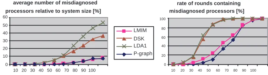
rate of rounds containing misdiagnosed processors [%]
0 20 40 60 80 100
10 20 30 40 50 60 70 80 90 100
average number of misdiagnosed processors relative to system size [%]
0 10 20 30 40 50 60
10 20 30 40 50 60 70 80 90 100
LMIM
DSK LDA1 P-graph
Fig. 7.2.Comparison of probabilistic diagnostic algorithms
area of local information diagnosis. It can be seen on the diagrams in Figure 7.2 that only the LMIM-algorithm approximates the accuracy of P-graph-algorithm.
8. Conclusions. Application of P-graph based modeling to system-level diagnosis provides a general framework that supports the solution of several different types of problems, that previously needed numerous different modeling approaches and solution algorithms. The representational power of the model was illustrated in this paper via some practical examples.
Another advantage of the P-graph models is that it takes into consideration more properties of the real system than previous diagnostic models. Therefore its diagnostic accuracy is also better. This means that it provides almost good diagnosis even when half of the processors are faulty, which is important in the field of wafer scale testing.
The favorable properties of the approach are achieved by considering the diagnostic system as a structured set of hypotheses with well-defined relations. The syndrome-decoding problem in multiprocessor systems has a special structure, namely the direct manifestation of internal fault states in the syndromes. In more complex systems the states of the control logic have to be taken into account in the model to be analyzed [21]. These straightforward extensions to the modeling of integrated diagnostics can be well incorporated into the P-graph based models. Our current work aims at generalization of the results into this direction by extending previous results on the qualitative modeling of dependable systems with quantitative optimization [22].
Acknowledgments. This research was supported by the Hungarian National Science Fund grant OTKA T032408, which is gratefully acknowledged by the authors.
REFERENCES
[1] T. Bartha, E. Sel´enyi,Probabilistic System-Level Fault Diagnostic Algorithms for Multiprocessors, Parallel Computing, vol. 22, no. 13, pp. 1807–1821, Elsevier Science, 1997.
[2] T. Bartha,Efficient System-Level Fault Diagnosis of Large Multiprocessor Systems, Ph.D thesis, BME-MIT, 2000. [3] M. Barborak, M. Malek, and A. Dahbura,The Consensus Problem in Fault Tolerant Computing, ACM Computing
Surveys, vol. 25, pp. 171–220, June 1993.
[4] T. Bartha, E. Sel´enyi,Probabilistic Fault Diagnosis in Large, Heterogeneous Computing Systems, Periodica Polytechnica, vol. 43/2, pp. 127–149, 2000.
[5] B. Polg´ar, Sz. Nov´aki, A. Pataricza, F. Friedler, A Process-Graph Based Formulation of the Syndrome-Decoding Problem, DDECS 2001, 4th Workshop on Design and Diagnostics of Electronic Circuits and Systems, pp. 267–272, Hungary, 2001.
[6] S. N. Maheshwari, S. L. Hakimi,On Models for Diagnosable Systems and Probabilistic Fault Diagnosis, IEEE Transactions on Computers, vol. C-25, pp. 228–236, 1976.
[7] B. Polg´ar, T. Bartha, E. Sel´enyi,Modeling Uncertainty In System-Level Fault Diagnosis Using Process Graphs, DAPSYS 2002, 4th Austrian-Hungarian Workshop on Distributed and Parallel Systems, pp. 195–200, Linz, Austria, Sept 29–Okt 2, 2002.
[8] M. L. Blount,Probabilistic Treatment of Diagnosis in Digital Systems, in Proc. of 7th IEEE International Symposium on Fault-Tolerant Computing (FTCS-7), pp. 72–77, June 1977.
[9] F. Friedler, K. Tarjan, Y. W. Huang, L. T. Fan,Combinatorial Algorithms for Process Synthesis, Comp. in Chemical Engineering, vol. 16, pp. 313–320, 1992.
[10] F. Friedler, K. Tarjan, Y. W. Huang, and L. T. Fan,Graph-Theoretic Approach to Process Synthesis: Axioms and Theorems, Chemical Engineering Science, 47(8), pp. 1973–1988, 1992.
[11] F. Friedler, L. T. Fan, and B. Imreh,Process Network Synthesis: Problem Definition, Networks, 28(2), pp. 119–124, 1998.
[12] F. Aglietti, et al., Self-Diagnosis of APEmille, Proc. EDCC-2 Companion Workshop on Dependable Computing, pp. 73–84, Silesian Technical University, Gliwice Poland, May 1996.
[13] A. Petri, P. Urb´an, J. Altmann, M. Dal Cin, E. Sel´enyi, K. Tilly, A. Pataricza,Constraint-Based Diagnosis Algorithms for Multiprocessors, Periodica Polytechnica Ser. El. Eng., Vol. 40, No. 1, (1996), pp. 39-52.
[14] S. Lee and K. G. Shin,Optimal multiple syndrome diagnosis, Digest of Papers, FTCS-20, Newcastle Upon Tyne, United Kingdom, pp. 324–331, June 1990.
[15] B. Sallay, P. Maestrini, P. Santi,ComparisonBased Wafer-Scale Diagnosis Tolerating Comparator Faults, IEEE Journal on Computers and Digital Techniques, 146(4), pp. 211–215, 1999.
[16] S. Chessa, Self-Diagnosis of Grid-Interconnected Systems, with Application to Self-Test of VLSI Wafers, Ph.D. Thesis, TD-2/99 University of Pisa, Italy, March 1999.
[17] M. Malek,A comparison connection assigment for diagnosis of multiprocessor systems, Proc. 7th FTCS, pp. 31-35, May 1980.
[18] K.Y. Chwa, S.L. Hakimi, Schemes for fault tolerant computing: a comparison of modulary redundant and tdiagnosable systems, Information and Controls, vol. 45, No. 3, pp. 212-238, 1981.
[20] A. Dahbura, K. Sabnani, and L. King,The Comparison Approach to Multiprocessor Fault Diagnosis, IEEE Transactions on Computers, vol. C-36, pp. 373–378, Mar. 1987.
[21] A. Pataricza, Algebraic Modelling of Diagnostic Problems in HW-SW Co-Design, in Digest of Abstracts of the IEEE International Workshop on Embedded Fault-Tolerant Systems, Dallas, Texas, Sept. 1996.
[22] A. Pataricza,Semi-decisions in the validation of dependable systems, Proc. of IEEE International Conference on Dependable Systems and Networks, pp. 114–115, G¨oteborg, Sweden, July 2001.
Edited by: Zsolt Nemeth, Dieter Kranzlmuller, Peter Kacsuk, Jens Volkert Received: April 1, 2003