A Self-Organizing Diffusion Mobile Adaptive Network
for Pursuing a Target
Amir Rastegarnia1,*, Azam Khalili1, Md Kafiul Islam2
1
Department of Electrical Engineering, University of Malayer, Malayer, Iran 2
Department of Electrical and Computer Engineering, National University of Singapore, Singapore
Abstract
In this paper we focus on designing self-organizing diffusion mobile adaptive networks where the individual agents are allowed to move in pursuit of an target. The well-known Adapt-then-Combine (ATC) algorithm is already available in the literature as a useful distributed diffusion-based adaptive learning network. However, in the ATC diffusion algorithm, fixed step sizes are used in the update equations for velocity vectors and location vectors. When the nodes are too far away from the target, such strategies may require large number of iterations to reach the target. To address this issue, we suggest two modifications on the ATC mobile adaptive network to improve its performance. The proposed modifications include (i) distance-based variable step size adjustment at diffusion algorithms to update velocity vectors and location vectors, (ii) to use a selective cooperation, by choosing the best nodes at every iteration, to reduce the number of communications. The performance of the proposed algorithm is evaluated by simulation tests where the obtained results show the superior performance of the proposed algorithm in comparison with the available ATC mobile adaptive network.Keywords
Adaptive networks, Mobile networks, LMS, Sensor networks1. Introduction
Wireless sensor networks appear in many practical applications such as distributed sensing, intrusion detection and target localization [1-4]. In most of the aforementioned applications, nodes of a network collect data from environment and then process them collaboratively to estimate a desired parameter. Different strategies have been introduced in the literature to solve the distributed estimation problems including consensus strategies and adaptive networks [5, 6]. It has been shown in [7] that adaptive networks are more stable than consensus networks and they provide better steady-state error performance. So, in this paper we focus on adaptive network based solutions. We adopt the term adaptive networks from [8] to refer to a collection of nodes that interact with each other and function as a single adaptive entity that is able to track statistical variations of data in real-time.
Two major classes of adaptive networks are incremental strategy [9-14] and diffusion strategy [15-19]. In comparison, incremental algorithms require less communication among nodes of the networks while diffusion algorithms are scalable and more robust to link and node failure [20-22].
In general, diffusion based algorithms consist of two
* Corresponding author:
[email protected] (Amir Rastegarnia) Published online at http://journal.sapub.org/ajsp
Copyright © 2016 Scientific & Academic Publishing. All Rights Reserved
steps including the adaptation step, where the node updates the weight estimate using local measurement data, and the combination step where the information from the neighbours are aggregated. Based on the order of these two steps, diffusion algorithms can be categorized into two classes known as the Combine-then-Adapt and Adapt-then-Combine (ATC). It is observed that the ATC version of diffusion LMS outperforms the CTA algorithm [16]. The initial diffusion adaptive networks in [15-19] did not incorporate the node mobility. In [23-26], another dimension of complexity which is node mobility has been added to the diffusion networks. The resultant mobile adaptive networks perform two diffusion-based estimation tasks: one for estimating the location of a target and the other one for tracking the center of mass of the network. Incorporating the node mobility enables the resulting diffusion networks to use them in new applications such as modelling the various forms of sophisticated behaviour exhibited by biological networks [27, 28] and source localization [29, 30].
target information, e.g. using bigger step-sizes when they are too far from the target. To endow the ATC diffusion network with such ability, we firstly define a practical metric to describe the far field region as a region that is too far from the target. Note that the near filed is also defined as a region that includes the target. Then, according to the position of a node (inside or outside of the far field) different step size adjust mechanisms are applied. In general, as long as a node is inside the far field region, the step size parameter in update velocity vectors and location vectors are increased, whereas for a node outside of the far field the step size is iteratively reduced as it moves toward the target.
Moreover, in the combination step of diffusion LMS algorithm, each node needs to gather the intermediate estimates from all of its neighbours. Thus, this step may require large amount of communications for dense networks. In some applications, however, networks cannot afford large communication overhead. To further reduce the communication load, a selective cooperation is used where every nodes selects only a subset of its niobous to share the information. The performance of the proposed algorithm is evaluated by simulation tests where the obtained results show the superior performance of the proposed algorithm in comparison with the available ATC adaptive network.
Notation: We use boldface letters for matrices and vectors
and small letters for scalars. The notation
|| ||
x
2=
x x
∗ stands for the Euclidean norm ofx
. E denotes the expectation operator. The set of neighbours of nodek , including itself, is denoted by
k.2. Mobile Adaptive Networks
Let us consider a network with N mobile nodes that are randomly distributed over a space. Let
x
k i, be the locationof node k at time i, relative to some global coordinate system and
w
o∈
3 denote the location of the target. Each node k finds its neighbours within a range R radius in each time i, i.e., ,
if ||
||
k j i k i
j
∈
x
−
x
≤
R
(1)The objectives of each node in the network are (i) to estimate the position of the desired target and move towards it in coherence and synchrony with the other nodes, and (ii), avoid possible collisions by keeping a certain distance, say
r
from neighbours during the motion to the target location. The distance between the targetw
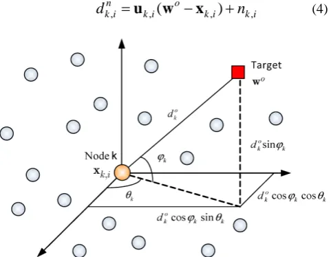
o and a node k at any time i is given by (See Fig. 1), ,
(
,)
o o
k i k i k i
d
=
u
w
−
x
(2)where
u
k i, denotes the direction of the target including theazimuth angle
θ
k i, , and the elevation angleϕ
k i, which is given as, [cos( ,) cos( ,) sin( ,) cos( ,) sin( ,)]
k i = θk i ϕk i θk i ϕk i ϕk i
u (3)
We assume that each node observes a noisy measurement of the distance to the target, via a linear model as follows
, ,
(
,)
,n o
k i k i k i k i
d
=
u
w
−
x
+
n
(4)Figure 1. Distance and direction of the target wo from node k at location xk i,
where
n
k i, denotes the noise term which is assumed to bezero-mean Gaussian noise. Intuitively, the noise variance,
2 ,
( )
n ki
σ
can follow a relation such as2 2
,
( )
,o
n k
i
k iσ
≈
κ
‖
x
−
w
‖
(5)We select
κ
=0.01 as [23]. Note that (5) is reasonable since we usually assume the signal power to decrease in proportional to the square of the propagation distance. We can rewrite the above equation as [23, 25], , , , , ,
n o
k i k i k i k i k i k i
d
=
d
+
u x
=
u w
+
n
(6)At every time instant i, every node k has access to local data
{
d
k i,,
u
k i,}
and the local data from its neighbours. Using these data every node estimates theposition of the target at
w
o which can be achieved by solving the following optimization problem2
, ,
1
arg min
(
)
N
k i k i
k
E d
=
−
∑
w
u w
(7)The ATC diffusion algorithm has been developed for solving (7) in a distributed manner. The ATC algorithm consists of two steps: adaptation and combination. In adaptation step, node k uses its own data to update the weight estimate
w
k i, 1− to intermediate valuem
k i, . In the combination step each node gathers the intermediate estimates{
m
,i},
∈
k combines them to obtain the updated weight estimatew
k i, . The algorithm is described as(
)
, , 1 , , , , , 1
k
w T
k i k i k k i i i k i
N c d
µ
− − ∈ = +∑
−m w u u w
(8)
, , ,
k w
k i k i
N a
∈
=
∑
w m
(9)
where
µ
k is the learning step size. The two sets ofnon-negative real coefficients
{
c
w,k}
and{
,}
wk
a
satisfy, , , ,
1 1
1,
0,
N N
w w w w
k k k k k
c
a
c
a
= =
=
=
=
=
∉
∑
∑
(10)In a network of mobile nodes, every node k can update its location as
, , 1 ,
k i
=
k i−+
k i∆
t
x
x
v
(11)where ∆t is the time step and
v
k i, 1+ denoted the velocityof the node k . Every node adjusts its velocity vector according to the following expression [23]
, 1 , 1
, 1 2 , 1
, 1 , 1
, ,
3 \{ } , ,
, ,
( )
k
k i k i g
k i k i
k i k i
l i k i
l k l i k i
l i k i
r
ξ
ξ
ξ
− − − − − ∈ − = + − − + − − −∑
w x v v w x x x x x x x ‖ ‖ ‖ ‖ (12)where
ξ
1,ξ
2 andξ
3 are non-negative weighting factors,and
v
gk i, is the local estimate for the global velocity of thecenter of gravity of the network which is designed to allow for coherent motion. To use (12) each node needs to estimate
, g k i
v
in a distributed way. Since the velocities of nodes arechanging in time, we need to keep track of
v
gk i, over time.So we introduce the global cost function as follows
2 , 1
arg min
g(
)
N g k i k
E
=
−
∑
v
v
v
(13)Similar to (8) we can arrive at the following diffusion algorithm for estimating
v
gk i,(
)
, , 1 , , , 1
k
g v g
k i k i k k i k i
N
c
δ
− − ∈=
+
∑
−
s
v
v
v
(14)
, = , ,
k
g v
k i k i
N a
∈
∑
v s
(15)
where
δ
k is a positive step size and{
c
v,k}
and{
a
v,k}
are two sets of non-negative real coefficients satisfying the same properties as (10).3. Proposed Algorithm
3.1. Motivation for Current Work
In the existing algorithms for adaptive mobile networks,
there is no specific strategy for going faster toward the target. In other words, in the existing algorithms although the algorithm is designed in such a way that the set of nodes can move towards the goal harmoniously, but they do not consider the distance to the target in their velocity and location update equations. To address this issue, instead of using fixed learning parameter
µ
k in (8), we use variable step-size parameter which has the following conditions● if node k at iteration i is too far from the target,
, k i
µ
should be increased. Note that to prevent algorithm divergence and movement control of the set of nodes, we have to select the upper limit for step-size parameters.● if distance of node k at iteration ibecomes less than a predefined value,
µ
k i, should be iteratively decreased as nodes approach the target. In this case we consider a lower bound forµ
k i, to avoid slow convergence rate.3.2. Algorithm Development
To begin with, we define the far field region as follows.
Definition 1: By far field, we mean a region
∈
3that the nodes inside it are far from the target, or
2 ,
|
||
w
o−
x
k i|
s
,
(16) To use (16), every node needs to have the target positiono
w
which is not available. To have a practical metric, weuse
w
k i, as an estimate ofw
o at iteration i and rewrite (16) as2
, ,
|
|
w
k i−
x
k i|
|
s
,
(17)For a node inside (i.e.
x
k i,∈
) a bigger step-size inthe update equation is required to move in the direction of
o
w
. So we replaceµ
k i, in (8) as follows, , 1
k i k i
µ
=
αµ
− (18)with
α
>1. Obviously, in this case we haveµ
k i,>
µ
k i, 1− .It should be noted that according to the recursive equation in (8), increasing the step size may lead to algorithm divergence. So, in order to avoid algorithm divergence we consider an upper bound for step sizes as
, 1 , 1 max
, ,
max , 1 max
(if
)
k i k i
k i k i
k i
αµ
αµ
µ
µ
µ
−αµ
−−µ
<
=
∈
≥
x
(19)When
x
k i,∉
we need to reduce the step size as nodesmoves toward the target at
w
o. In this case the step size adaptation function can be given by2
, , 1
( )
k i k i
e i
kwhere
e i
k( )
=
d i
k( )
−
u
k i,(
w
k i, 1−−
x
k i, 1−)
. In this case, k i
µ
becomes smaller as node approaches the target. To avoid slow convergence rate, we can consider a lower bound for step size as follows2
, 1 , 1 min
, 2 ,
min , 1 min
( )
(if )
( )
k i k i k
k i k i
k i k
e i e i αµ βµ γ µ µ µ βµ γ µ − − −
+ >
= ∉
+ ≤
x (21)
As mentioned in the introduction, in some applications, networks cannot afford large communication overhead due to energy consumption cost or bandwidth restrictions. In order to minimize the communication overhead for this application, we must introduce a new metric that considers only a subset of neighbours to consult at node k. To this end, we select neighbours of node k that have small
estimated variance product measure and ignore the other neighbours. One way is to change (1) as
2 2
, , , ,
||
|
if
|
an
d
k j i k i j i k i
j
∈
x
−
x
≤
R
σ
≤
σ
(22)Remark 1: To use (22) we need
σ
k i2, which are unknown in general and for practical usage they must be estimated. At every node k,σ
k i2, can be estimated by time-averaging as2 2
, , 1 , , 1
ˆ
k iˆ
k i(1
)(
d i
k( )
k i k i)
σ
=
ησ
−+ −
η
−
u w
− (23)with a forgetting factor
0
< <
η
1
.Finally, using the introduced modifications we arrive at the proposed algorithm as given in the Table. 1.
Table 1. Proposed Diffusion Mobile Adaptive Network with Selective Cooperation
Every node k in the network performs the following steps for i>0. The node has access to the local data {dk( ),i uk i, ,vk i, ,σn k2, } If ||wk i, −xk i, ||2s then
, 1 , 1 max
, ,
max , 1 max
(if )
k i k i
k i k i
k i αµ αµ µ µ µ αµ µ − − − < = ∈ ≥
x 2
, 1 , 1 min
, 2 ,
min , 1 min
( )
(if )
( )
k i k i k
k i k i
k i k e i e i αµ βµ γ µ µ µ βµ γ µ − − − + > = ∉ + ≤
x Use (22) to find set of neighbour nodes of every node k (i.e. k i, ) Compute the following local adaptation and criterion
(
)
(
)
, , 1 , , , , , 1
, , 1 , , , 1
k
k
w T
k i k i k k i i i k i N
g v g
k i k i k k i k i N c d c µ δ − − ∈ − − ∈ = + − = + −
∑
∑
m w u u w
s v v v
Perform two local combination steps using data from selected neighbours
, , , , , ,
k k
w g v
k i k i k i k i
N N
a a
∈ ∈
=
∑
=∑
w m v s
Update the node velocity and its location
, 1 , 1
, 1 2 , 1
, 1 , 1
, ,
3 \{ } , ,
, ,
, , 1 ,
(| ||
|
| )
|| |
k
k i k i g
k i k i
k i k i
l i k i l k l i k i
l i k i
k i k i k i
r t ξ ξ ξ − − − − − ∈ − − = + − − + − − − = + ∆
∑
w x v v w x x x x x x xx x v
4. Simulation Results
In this section we present simulation results to evaluate the performance of our proposed algorithm. We use a network with N=50 nodes that are initially uniformly distributed inside a cube with length 10. Their velocities are set at random directions and unit magnitude. The simulation parameters are set as follows. The factors of velocity control are ξ =1 0.8 , ξ =2 0.5 , ξ =2 0.8 . We further set
0.85, 0.001
β= γ = . The combination coefficients are set
as
a
l kw,=
a
l kv,=
c
l kw,=
c
l kv,=
1/ |
k( ) |
i
ifl
∈
k( )
i
. We set the time duration to ∆ =t 0.5 andδ
=0.5
. Moreover, optimal distance between two neighbours is set to2
r= . A node chooses nearest neighbours from neighbours within the radius R=6. The observation noise
n i
k( )
is assumed to be zero-mean Gaussian noise which is given by (5).Figure 2. Transient network MSD for estimating the target location at
[120 120]
o = T
w
Fig. 2 shows the network transient mean-square deviation (MSD) (for two different algorithms) which is defined as
2 , 1
1
MSD
[|
|
|
|
]
N
o
i k i
k
E
N
==
∑
w
−
w
(24)In the following, we compare the performance of the proposed algorithm with the ATC algorithm given in [25]. Note that for the ATC algorithm each node cooperates with fixed number of its nearest neighbours at every iteration (
k i,=
4
). Moreover, each node uses fixed step-size0.5
kµ
=
at every iteration. Fig. 2 shows the transient network MSD for estimating the target location at[120 120]
o
=
Tw
. These curves are averaged over 50experiments with the same initial state of
w
k, 1− for all k.We observe that for both algorithms the transient MSD decreases dramatically in the first phase, then the network moves towards the target and finally, at steady state, the
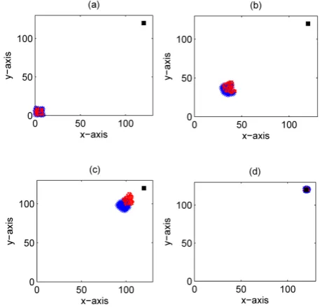
network arrives at the target. However, the proposed algorithm provides better performance compared to the ATC diffusion algorithm. Fig. 3 illustrates the maneuver of a mobile network (with ATC and proposed algorithms) over time.
Figure 3. Maneuvers of mobile networks (with the ATC and the proposed algorithms) over time. (a)i=1, (b)i=50 , (c)i=150 , and (d)
300
i= . Note that * and
•
indicates the locations and moving directions of the nodes with ATC, proposed algorithm respectively and denotes the location of the targetFigure 4. The network average step size µk i, over iteration
We observe that both algorithms exhibits harmonious movement, but the proposed algorithm moves faster to the target. Fig. 4 shows how the network average step size, i.e.
, ,
1
1
Nk i k i
k
N
µ
µ
=
=
∑
some iterations we have
µ
k i,=
µ
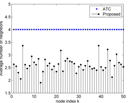
max. As the nodes move toward the target, at every node the step size parameter has been decreased iteratively.Fig. 5 shows the average number of neighbours for every node. Note that for the ATC algorithm we have
k i,=
4
(according to our simulation setup) while the proposed algorithm uses small number of neighbours which means it requires less communication load.
Figure 5. The average number of neighbours for every node
5. Conclusions
In this paper we proposed a modified ATC diffusion algorithm for mobile adaptive networks where the individual agents are allowed to move in pursuit of a target. The motivation was that in the ATC algorithm fixed step sizes are used in the update equations for velocity vectors and location vectors. When the nodes are too far away from the target, such strategies may require large number of iterations to reach the target. To address this issue, in the proposed algorithm we used distance-based variable step sizes for adjustment at diffusion algorithms to update velocity vectors and location vectors. We also used a selective cooperation where only a subset of nodes at each iteration is used to share information. The performance of the proposed algorithm was evaluated by simulation tests where the obtained results showed the superior performance of the proposed algorithm in comparison with the available ATC mobile adaptive network. In our future work we will develop diffusion mobile adaptive network for pursuing multiple targets.
REFERENCES
[1] D. Estrin, G. Pottie, and M. Srivastava, Instrumenting the world with wireless sensor networks, in Proc. Int. Conf. Acoustics, Speech, Signal Processing (ICASSP), Salt Lake City, UT, May 2001, pp. 2033-2036.
[2] H Leung, S Chandana, and S Wei, Distributed sensing based on intelligent sensor networks, IEEE Circuits and Systems, Mag., vol. 8, no. 2, pp. 38-52, May 2008.
[3] R. P. Yadav, P. V. Varde, P. S. V. Nataraj et al. Model-based tracking for agent-based control systems in the case of sensor failures, International Journal of Automation and Computing, 2012, 9(6): 561-569.
[4] Chao-Lei Wang, Tian-Miao Wang, Jian-Hong Liang et al. Bearing-only visual SLAM for small unmanned aerial vehicles in GPS-denied environments, International Journal of Automation and Computing, 2013, 10(5): 387-396. [5] A. H. Sayed, Adaptation, learning, and optimization over
networks, Foundations and Trends in Machine Learning, vol. 7, issue 4-5, pp. 311-801, NOW Publishers, Boston-Delft, 2014.
[6] A. H. Sayed, Adaptive networks, Proceedings of the IEEE, vol. 102, no. 4, pp. 460-497, April 2014.
[7] S.-Y. Tu and A. H. Sayed, Diffusion strategies outperform consensus strategies for distributed estimation over adaptive networks, IEEE Trans. Signal Processing, vol. 60, no. 12, pp. 6217-6234, Dec. 2012.
[8] A. H. Sayed and C. Lopes, Distributed recursive least-squares strategies over adaptive networks, in: Proc. 40th Asilomar Conf. on Signals, Systems and Computers, Pacific Grove, CA, Oct. 2006, pp. 233-237.
[9] C. G. Lopes and A. H. Sayed, Incremental adaptive strategies over distributed networks, IEEE Trans. on Signal Process., vol. 55, no. 8, August 2007, pp. 4064-4077.
[10] N. Takahashi and I. Yamada, Incremental adaptive filtering over distributed networks using parallel projection onto hyperslabs, IEICE Technical Report, vol. 108, pp. 17-22, 2008.
[11] T. Panigrahi and G. Panda, Robust distributed learning in wireless sensor network using efficient step size, in 2nd International Conference on Communication Computing and Security at NIT Rourkela, India, 06-08 October 2012, Procedia Technology 6 (2012), pp. 864-871.
[12] G. Azarnia, M. A. Tinati, Steady-state analysis of the deficient length incremental LMS adaptive networks with noisy links, AEU - International Journal of Electronics and Communications, Volume 69, Issue 1, January 2015, Pages 153-162.
[13] A. Khalili, A Rastegarnia, WM Bazzi, Incremental augmented affine projection algorithm for collaborative processing of complex signals, 2015 International Conference on Information and Communication Technology Research (ICTRC), 60-63, 2015.
[14] W. M. Bazzi, A. Rastegarnia, and A. Khalili, A Quality-aware Incremental LMS Algorithm for Distributed Adaptive Estimation, International Journal of Automation and Computing, vol. 11, no. 6, pp. 676-682, 2015.
[15] C. G. Lopes and A. H. Sayed, Diffusion least-mean squares over adaptive networks: Formulation and performance analysis, IEEE Trans. Signal Process., vol. 56, no. 7, pp. 3122-3136, Jul. 2008.
Processing, vol. 58, no. 3, pp. 1035-1048, March 2010. [17] J. Chen and A. H. Sayed, Diffusion adaptation strategies for
distributed optimization and learning over networks, IEEE Trans. Signal Process., vol. 60, no. 8, pp. 4289-4305, Aug. 2012.
[18] A. H. Sayed, S.-Y. Tu, J. Chen, X. Zhao, and Z. Towfic, Diffusion strategies for adaptation and learning over networks, IEEE Signal Process. Mag., vol. 30, no. 3, pp. 155-171, May 2013.
[19] X. Zhao and A. H. Sayed, Distributed clustering and learning over networks, IEEE Trans. Signal Process., vol. 63, no. 13, pp. 3285-3300, July 2015.
[20] A. Khalili, M. A. Tinati, A. Rastegarnia, and J. A. Chambers, Steady-state analysis of diffusion LMS adaptive networks with noisy links, IEEE Trans. Signal Process., vol. 60, no. 2, pp. 974-979, Feb. 2012.
[21] A. Rastegarnia, W. M. Bazzi, A. Khalili and J. A. Chambers, Diffusion adaptive networks with imperfect communications: link failure and channel noise, IET Signal Processing, vol. 8, no. 1, pp.59-66, 2014.
[22] X. Zhao, S.-Y. Tu, and A. H. Sayed, Diffusion adaptation over networks under imperfect information exchange and non-stationary data, IEEE Trans. on Signal Process., vol. 60, no. 7, pp. 3460-3475, July 2012.
[23] S.-Y. Tu and A. Sayed, Mobile adaptive networks with selforganization abilities, in Wireless Communication Systems (ISWCS), 2010 7th International Symposium on, Sept 2010, pp. 379-383.
[24] S.-Y. Tu and A. Sayed, Tracking behavior of mobile adaptive
networks, in Signals, Systems and Computers (ASILOMAR), 2010 Conference Record of the Forty Fourth Asilomar Conference on, Nov 2010, pp. 698-702.
[25] S.-Y. Tu and A. Sayed, Mobile adaptive networks, Selected Topics on Signal Processing, vol. 5, no. 4, pp. 649-664, August 2011.
[26] May Zar Lin, Manohar N. Murthi and Kamal Premaratne, Mobile adaptive networks for pursuing multiple targets, in Proc. Int. Conf. Acoustics, Speech, Signal Processing (ICASSP)}, Brisbane, Australia, 2015, pp. 3217-3221. [27] F. Cattivelli and A. H. Sayed, Modeling bird flight formations
using diffusion adaptation, IEEE Trans. Signal Process, vol. 59, no. 5, pp. 2038-2051, May 2011.
[28] J. Li and A. H. Sayed, Modeling bee swarming behavior through diffusion adaptation with asymmetric information sharing, EURASIP Journal on Advances in Signal Processing}, vol. 2012, no. 18, January 2012.
[29] J.-G. Li, Q.-H. Meng, Y. Wang, and M. Zeng, Odor source localization using a mobile robot in outdoor airflow environments with a particle filter algorithm, Autonomous Robots, vol. 30, no. 3, pp. 281-292, 2011.
[30] A. Khalili, A. Rastegarnia, M. Islam, and Z. Yang, A bio-inspired cooperative algorithm for distributed source localization with mobile nodes, in Engineering in Medicine and Biology Society (EMBC), 35th Annual International Conference of the IEEE, July 2013, pp. 3515-3518.