Buoyancy Term Evolution in the Multi Relaxation Time Model of Lattice Boltzmann Method with Variable Thermal Conductivity Using a Modified Set of Boundary Conditions

Please cite this article as: M. Varmazyar, A. Mohammadi, M. Bazargan, M. A. D. Hosseini, Buoyancy Term Evolution in the Multi Relaxation Time Model of Lattice Boltzmann Method with Variable Thermal Conductivity Using a Modified Set of Boundary Conditions, International Journal of Engineering (IJE), TRANSACTIONS C: Aspects Vol. 30, No. 9, (September 2017) 1408-1416

International Journal of Engineering

J o u r n a l H o m e p a g e : w w w . i j e . i r

Buoyancy Term Evolution in the Multi Relaxation Time Model of Lattice Boltzmann

Method with Variable Thermal Conductivity Using a Modified Set of Boundary

Conditions

M. Varmazyar*a_{, A. Mohammadi}a_{, M. Bazargan}b

a _{Department of Mechanical Engineering, Shahid Rajaee Teacher Training University, Tehran Iran} b _{Department of Mechanical Engineering, K. N. Toosi University of Technology, Tehran, Iran}

P A P E R I N F O

Paper history: Received 12 March 2017

Received in revised form 07May 2017 Accepted 07 July 2017

Keywords:

Lattice Boltzmann Method Boundary Condition Multi Relaxation Time Variable Thermal Conductivity Rayleigh-Benard Convection

A B S T R A C T

During the last few years, a number of numerical boundary condition schemes have been used to study various aspects of the no-slip wall condition using the lattice Boltzmann method. In this paper, a modified boundary condition method is employed to simulate the no-slip wall condition in the presence of the body force term near the wall. These conditions are based on the idea of the bounce-back of the non-equilibrium distribution. The error associated with the modified model is smaller than those of other boundary condition models available in the literature. Additionally, various schemes to simulate body forces have been studied. Based on the numerical results, the model demonstrating minimum error has been reported. Finally, it has been shown that the present model is capable of simulating the effect of high nonlinearity in the heat transfer equation in the presence of a variable thermal conductivity. This has been accomplished by employing a multi relaxation time scheme to model a Rayleigh-Benard natural convection current in a 2-D domain with high Rayleigh numbers. Previous studies reported that the onset of oscillation occurs at Ra≈30,000 and Pr=6.0. By the modified boundary condition method which is used in this study, the oscillation is removed until at least Ra≈ 45,000 and Pr=6.0. The results show that applying scheme 3 for the current boundary condition yields the least amount of error compared to the semi-empirical correlation. The Rayleigh-Benard convection problem has been revisited in the presence of a variable thermal conductivity and the simulation results

remain stable for flows with a large variation of thermal conductivity ( = 0.7) and Rayleigh numbers up to 1,000,000 and Pr=0.7.

doi: 10.5829/ije.2017.30.09c.14

1. INTRODUCTION1

Conventional methods in computational fluid dynamics (CFD) are based on the direct discretization of conservation equations [1, 2]. These methods have a macroscopic view in dealing with fluid dynamics problems [3, 4] and are widely used in the simulation of physical transport phenomena [5, 6]. Alternatively, the kinetic methods for CFD, such as the lattice Boltzmann method, take a microscopic approach and are derived from the Boltzmann equation [7-10]. One particular application of the lattice Boltzmann method is the

*Corresponding Author’s Email: [email protected] (M. Varmazyar)

modeling of fluids under the influence of body forces [11]. Some examples of such flows are magneto-hydrodynamic [12] fluid flow, buoyancy driven flow [13, 14], multi-phase or multi-component fluid flows and the flow of non-ideal gases obeying a van der Waals type of equation of state [15].

Various schemes taking the body forces into account may be divided into three general categories. The first approach, called Scheme 1 in this study, is based on the suggestion of Luo [16] in which the effect of body forces are considered in the collision term as:

i ₂

1

F _{i i}.

s

w c F c



Another method, referred to as Scheme 2 in the current study, is based on the work of Shan and Chen [17]. In order to account for body forces, they employed Newton’s second law and modified the fluid and equilibrium velocities as follows:

( , ) ( , ) ( , ) F r t

u r t u r t 





  (2)

( , ) ( , ) ( , )

eq F r t

u r t u r t 





  (3)

It seems to be more accurate if both the collision term and the velocity equations are modified in order to account for external forces. This idea has been employed by Guo et al. [18] and forms what is called Scheme 3 in this study. This method leads to the same conservation equations reached by macroscopic solutions. To obtain the Navier-Stokes equations, Guo et al. [18] applied the following modifications in the force and velocity equations.

 

i _{2 4}

. 1

F 1 .

2

i i

i i

s s

c u

c u

w c F

c c



 _ 

 

 _{ }   

  _ _ (4)

( , ) ( , ) ( , )

2

F r t

u r t u r t





  (5)

( , ) ( , ) ( , )

2

F r t

u r t u r t





  (6)

More recently, Mohamad and Kuzmin [19] examined a good number of formulations suggested by various investigators to assess the accuracy of different schemes. They showed that the method of Guo et al. [18] is noticeably more accurate than those reported by others.

The buoyancy can be a good example for considering body forces in an LBM simulation. To analyze a buoyancy-driven flow, the temperature profile needs to be obtained. The thermal conductivity has been assumed to vary with temperature in this study. Hazi and Markus [20] employed Scheme 1 to study convective heat transfer to a supercritical fluid. The fluid thermal conductivity varied with the temperature near the critical region. More recently, Varmazyar and Bazargan [21] refined further details of the Hazi and Markus’s [20] model. They employed a Chapman-Enskog analysis and showed that this model is capable of simulating the effect of nonlinearity of the heat transfer equation due to the variation of thermal conductivity in the energy equation. Results with acceptable error were reported by Varmazyar and Bazargan [21] for a variety of heat conduction case studies. In addition to Scheme 1, it is worthwhile to try

Scheme 2 and Scheme 3 to investigate the accuracy of convective heat transfer simulations by comparison of errors generated in various schemes. This has been accomplished in the present study.

The force and velocity equations are modified in order to model the effect of body forces. The boundary conditions also need to be adjusted accordingly. The most common set of boundary conditions used in the LBM is the bounce-back model. In this type of boundary conditions, the particles bounce-back to the fluid nodes in opposite directions from which they strike the wall nodes. The set of boundary conditions may be categorized in terms of the order of magnitude of the error generated [22]. Since the accuracy of the LBM is of the second order inside the mesh points, the first order boundary conditions degrade the lattice Boltzmann method. Many attempts have been made to introduce higher order schemes for boundary conditions [23-27]. The bounce-back approach satisfies the mass conservation on the wall and assures the zero velocity on the boundary. However, a problem appears once the body forces are present. They may cause a jump in the distribution function on the boundary. This has also been addressed by Li and Tafti [28]. They showed that applying the common bounce-back boundary condition leads to an erroneous velocity jump at the wall in the presence of local forces due to liquid-vapor interactions. They developed a mass-conserving velocity-boundary condition in order to eliminate the unwanted velocity component. This matter deserves further investigations and has been extensively discussed in the current study.

To accomplish the goals mentioned above, the following steps are taken. First, the mathematical models for the fluid motion and the thermal heat transfer are presented. Then, numerical examples are applied to show the capability of the models. Next, the accuracy of the introduced boundary condition in the current study as well as various schemes used for body forces is evaluated in Poiseuille flow and Rayleigh-Benard convection case studies. Finally, the effect of variable thermal conductivity is investigated.

2. GOVERNING EQUATIONS AND MODELING

The LBM for an incompressible gas and corresponding thermal LBM have been described below. The variation of thermal diffusivity with temperature has been considered. Multi relaxation time scheme has been used to increase the stability and accuracy of the model.

i i i i

f ( + ,t+1)-f ( ,t)=r ci r +F (7)

where r, t and F_i are the location vector, time and body forces, respectively. The term f_i is the particle distribution function traveling with velocity c_i. The collision operator _i represents the rate of change of f_i due to collision of particles. The particle distribution after propagation is relaxed towards the equilibrium distribution eq

i

f ( , )r t . The formulation of the Bhatnagher-Gross-Krook method (BGK) [29] for collision operator has been used in this study as:

eq

i i i

1

(f ( , )r t f ( , ))r t



   (8)

The relaxation parameter  has been calculated from the kinematic viscosity  of the simulated fluid according to the following equation [30]:

1 3

2

  (9)

The equilibrium density f_ieq( , )r t is calculated as:





eq i

2

2 4 2

f ( , ) ( , )

. . . (1 ) 2 2 i eq

eq _i eq eq

i

s s s

r t w r t

c u

c u u u

c c c



 

  

(10)

where c_s is the speed of sound, and w_i is the corresponding equilibrium density for ueq0. Taking the moment of the distribution function, the density and microscopic velocity may be obtained as follows:

i i ( , )r t f ( , )r t

 

_

₍₁₁₎

i i 1

( , ) f ( , )

( , ) i

u r t r t c

r t



 

_

₍₁₂₎

The body force in the lattice Boltzmann model is calculated as below:



m



F   G (13)

where _m and G are the average fluid density and gravity acceleration, respectively. Using the Boussinesq approximation, the body force (buoyancy) term in Rayleigh-Benard convection will be:

( m)

F  TT G (14)

where T_m and  are the average fluid temperature and volumetric thermal expansion coefficients, respectively.

2. 2. Multi-relaxation Time Scheme A Multi-Relaxation Time (MRT) scheme has been applied in which the collision operator has the form of a diagonalizable matrix ij. The MRT collision operator interacts with equilibrium particle distribution functions as below:





i i

eq

j j i

f ( + ,t+1)-f ( ,t)

f ( ,t)-f ( ,t) +F i

ij j

r c r

r r



 



(15)

It has been claimed that the MRT scheme proposes a higher stability and accuracy than a single relaxation time scheme [30]. Hence, Equation (15) can be converted to the following equation:





i i

eq 1

j j i

f ( + ,t+1)-f ( ,t)

f ( ,t)-f ( ,t) +F i

r c r

M r r



  (16)

where f ( ,t)_j r and f_jeq( ,t)r are the vectors of the moment. The mapping between the distribution function and moment vectors can be stated by the linear transformation shown below:

f( ,t)r M f( ,t)r (17)

The Gram-Schmidt orthogonalization procedure may be employed to calculate the transformation matrix M. The general form of the transformation matrix has been suggested by Ginzburg [31]. Consequently, the transformation matrix M for a D2Q9 type of lattice using an MRT model is expressed as below [32]:

1 1 1 1 1 1 1 1 1

4 1 1 1 1 2 2 2 2

4 2 2 2 2 1 1 1 1

0 1 0 1 0 1 1 1 1

0 2 1 2 0 1 1 1 1

0 0 1 0 1 1 1 1 1

0 0 2 0 2 1 1 1 1

0 1 1 1 1 0 0 0 0

0 0 0 0 0 1 1 1 1

M            _{        }                          _       _          _{     }           _{   }    (18)

The relaxation matrix  used in Equation (14) is a diagonal matrix and is described as below [32]:

4 6

(0.0, 1.63, 1.14, , 1.92,

2 2

, 1.92, , )

1 6 1 6

DIAGONAL         (19)

1

feq, f₂eq 23



u u'. '



, f₃eq  3



u u'. '



,

4

fequ'_x, f₅eq u'_x, f₆equ'_y, f₇eq u'_y,





2





2

8

feq u'x  u'y , f9 2 ' ' eq x y u u   (20)

where u'_x and u'y are the components of microscopic velocity.

2. 3. Thermal LBM with Variable Thermal Diffusion Coefficient To simulate the energy equation with variable thermal conductivity, the general form of the LBE has been used. To account for variations of conductivity in the heat transfer equation, the equilibrium distribution function needs to be modified as below [21]:

i 2 2

1

g ( , )eq _{i i}. _i.

s s

D

r t w T c u c T

c c



 

 _    _

  (21)

where D is the variable part of the thermal conductivity and T is the temperature. The relaxation time () is related to the constant part of the diffusion coefficient with Equation (22):

0 2 1 1 2 s c

   ₍₂₂₎

where ₀ is the constant part of thermal diffusivity. The temperature is calculated by Equation (23):

i i

g ( , )

T



r t ₍₂₃₎

2. 4. Boundary Conditions For the Dirichlet boundary condition in thermal LBM, it is assumed that the flux is balanced in any direction (g_i geq_i g_jgeq_j ). The subscript i shows the direction of particles after being reflected back to the domain. Subscript j shows the corresponding mirror direction of particles. For nodes on the wall, the balanced flux can be written as

eq

i i

g (w_iw T_j)_wg in which Tw is the wall

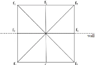
temperature. To simulate the zero velocity on the wall, a bounce-back type of boundary condition on the non-equilibrium part of the distribution function is implemented. Figure 1 is presented to explain the boundary condition used in the current study. The upper wall is coinciding with the x-axis and is shown by the dotted line in Figure 1. The unknown values of f4, f7 and

f8 pointing outwards with respect to the wall are to be

calculated by using the after streaming values of f0, f1,

f2, f3, f5, f6.

Supposing that u_x and u_y are given on the wall, Equations (24) are employed to determine f4, f7, f8 and ρ

[33].





4 7 8 0 1 2 3 5 6

f f f   f  f f f f f ,

4 7 8 2 5 6

f f f f f f

2 y y F u         ,

3 6 7 1 5 8

f f f f f f

2 x x F u         (24)

Simplifying Equations (24) yields Equation (25):





0 1 3 2 5 6

f f f 2 f f f

2 1 y y F u         (25)

From the bounce-back idea applied to the non-equilibrium part of the particle distribution normal to the boundary, it is understood that f₂f₂eqf₄f₄eq. This can convert the set of Equations (24) into a closed form as stated in Equations (26).

4 2

2 f f

3uy

  ,





7 5 1 3

1 1 1

f f f f

2 6 2 4 4

y x y x F F u u          ,





8 6 1 3

1 1 1

f f f f

2 6 2 4 4

y x y x F F u u          (26)

The advantage of the present approach in expressing boundary conditions is that various components of the force term have been taken into consideration and thus more continuity in values of the distribution function hold at the wall.

3. RESULTS AND DISCUSSION

Two numerical case studies are presented to illustrate the capabilities of the current model. In the first example, the three schemes mentioned earlier to account for body forces, together with the modified boundary condition have been examined in a Poiseuille flow. Errors associated with the solutions are compared. In the second example, a Rayleigh-Benard convection problem has been considered.

The accuracy and stability of the present simulation have been evaluated under various conditions. Furthermore, the effects of thermal conductivity variations have been investigated in this case study.

3. 1. Poiseuille Flow Case Study A Poiseuille flow driven by a forcing mechanism is an excellent example versus which the present model may be evaluated. That is because the analytical solution for such flow is known. The velocity profile obtained from the Navier-Stokes equations for incompressible Poiseuille flow is as follows:

2

0 2 1 y

y

u u

Ly

 _{ } 

 

 _{  }  _

 

 

(27)

where u₀F Ly_d 2



4



, Fd is the driving force and Ly

is the channel width. The change of error with channel width is to be examined. The grid resolutions from Ly=8 to Ly=64 have been tried. The Reynolds number

Re=u0Ly/υ has been kept constant. Since the kinematic viscosity depends only on τ, the product u0Ly needs to

remain constant. It means that if the channel width is doubled, u0 needs to be halved, and thus the forcing F is decreased eightfold. Zero velocity on the top and bottom boundaries is implemented according to boundary condition explained in the previous section. Inlet and outlet boundary conditions along the flow direction are set to be periodic.

The error in values of the predicted velocity of this study with respect to the results of the analytical solution is defined by Equation (28):





2

i i n

i

err



UN UE N ₍₂₈₎

where Nn is the number of points, and UEi and UNi correspond to the analytical and numerical normalized velocity for the ith node, respectively. Normalization is made by means of the velocity in the center of the channel.

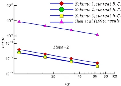
Figure 2 illustrates the error defined in Equation (28) versus the channel width. Apparently, the error decreases with the increase of channel width regardless of the numerical scheme used. The calculations determine that the slope of error variations with channel width for various results shown in Figure 2 is about -2, i.e., the second order. However, the results of this study provide smaller values of error compared to data of Chen et al. [22] by orders of magnitudes. Such improvement in the results is not due to modifications made to the scheme by which the body force is modeled. It can be seen that all three schemes used in this study lead to more or less the same results. In fact, the scheme used to model the body force by Chen et al. [22] is identical to what is called Scheme 1 in this study.

The smaller error obtained in the current study is, therefore, the result of more accurate modeling of the boundary condition. Chen et al. [22] have applied an extrapolation scheme to model the boundary condition.

3. 2. Rayleigh-Benard Convection Case Study

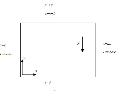
A two-dimensional simulation of steady Rayleigh-Benard natural convection as a benchmark has been used to evaluate the results of the present study. The schematic diagram of the flow between two parallel plates and the macroscopic boundary conditions are shown in Figure 3. As illustrated, the walls at y = 0 and

y = Ly are heated and cooled, respectively. Other walls are in periodic conditions. The fluid is initially at rest. Thermodynamic equilibrium at constant temperature T0

is maintained. T0 is the average of the heated and cooled

wall temperatures.

The variation of the thermal conductivity has been accounted for by a linear equation as expressed below:

 

0

 





0 0 1 bottom

p

k k T

D T T T

c

  

 

 

   _   _ (29)

where k T

 

,  and c_p are the thermal conductivity, density, and specific heat capacity, respectively. The D2Q9 is used to calculate the temperature distribution and velocity profiles.

To investigate the independence of the numerical solution from the number of grids, different lattice sizes from 31×61 to 151×301 are examined. It was found that there is no significant change in the results with a number of grids larger than 111×221. Simulations at various Rayleigh numbers are performed on an 111×221 lattice with a Prandtl number of 0.71. The simulation is started from the static conductive state, beginning with Ra=2,000. The Nusselt numbers calculated under the steady state conditions and constant diffusion coefficient are shown in Table 1.

Figure 3. Distribution function for D2Q9 configuration on the upper wall

TABLE 1. Nusselt number calculated by numerical schemes and semi-empirical correlation for a Rayleigh-Benard convection problem

Scheme used to model body force

Boundary condition modeling

Nusselt number

Ra=20,000 Ra=30,000

Scheme 3 First order

bounce-back 3.247 3.564

Scheme 3 Second order

bounce-back 3.210 3.565

Scheme 1 Current model 3.225 3.590

Scheme 2 Current model 3.980 4.394

Scheme 3 Current model 3.238 3.635

Semi empirical correlation:

1.56×(Ra/Rac)0.296 3.232 3.644

Two flows with different Rayleigh numbers are examined. The table contains the results obtained by different schemes for modeling body forces together with various models for boundary condition including the one used in this study. The results of a semi-empirical correlation, Nu=1.56×(Ra/Rac)0.296 with critical Rayleigh number (Rac) equal to 1707, are also presented for the sake of comparison. The results show that applying scheme 3 for the current boundary condition yields the least amount of error compared to the semi-empirical correlation.

The steady-state isotherms for a wide range of Rayleigh numbers are shown in Figure 4. As shown, when the Rayleigh number is increased, the thermal boundary layer thickness gets smaller. The rising and falling fluid layers become narrower. The Rayleigh number is increased to magnitudes as high as 1,000,000. Unlike the thermal LBE model [34], the present model remains numerically stable.

Shan [35] simulated the same problem with the bounce-back boundary condition. He found however that if the simulation is started from the static conductive state with Ra=50,000, the system will evolve into an oscillatory state. He reported that this oscillation occurs in simulations with Ra>30,000 with Pr=6.0. By the modified boundary condition method used, the oscillation is removed until at least Ra= 45,000 with Pr=6.0. It shows that the current method has more stability than the bounce-back method.

In the next step, the variation of thermal conductivity has been taken into account. The calculations have been carried out for various values of the thermal conductivity coefficient,  = 0.0, 0.1, 0.3 and 0.7. The Ra and Pr numbers are assumed to be 1,000,000 and 0.71, respectively.

The isotherms for various values of  are illustrated in Figure 5. The corresponding Nusselt number for

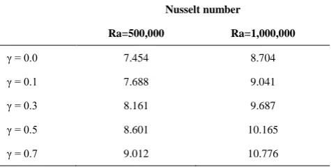
Ra=500,000 and Ra=1,000,000 is calculated in Table 2. As shown in Figure 5, an increase in the thermal conductivity coefficient makes the thermal boundary layer narrower. The high nonlinearity in the heat transfer equation causes the high-temperature region near the cold wall larger. Results show that the current thermal LBM can model highly nonlinear energy equations satisfactorily.

Acording to the results of this study, by increasing , the circulation of the vortex increases and this leads a rise in the velocity of the cold and hot fluids. In other words, the cold flow travels faster towards the bottom wall. Meanwhile, a part of the cold flow is separated by the twin vortices and is driven upward so that a circulatory pattern resumes. As the vortex intensity enhances by the rise of thermal conductivity coefficient, the greater part of hot and cold fluids are mixed. It yields an increase in the Nusselt number.

Figure 5. Two-dimensional simulation Isotherms at steady states for Ra=1,000,000 with variation of thermal conductivity

TABLE 2. Nusselt number values calculated by numerical scheme with variation of thermal conductivity

Nusselt number

Ra=500,000 Ra=1,000,000

γ = 0.0 7.454 8.704

γ = 0.1 7.688 9.041

γ = 0.3 8.161 9.687

γ = 0.5 8.601 10.165

γ = 0.7 9.012 10.776

4. CONCLUSIONS

To decrease the error associated with the boundary condition method, a modified no-slip wall condition model has been implemented. The body force term near the wall has been taken into account. The results show that the current boundary condition model is more accurate than the available methods in the literature. By using the method of current study, the steady-state Rayleigh-Benard convection for a wide range of Rayleigh numbers has been simulated. Results show that the present method can eliminate the oscillations and provides more stable solutions for natural convection flows with Rayleigh numbers up to 45,000. Additionally, it has been illustrated that the current method is capable of simulating the effect of high nonlinearity in the heat transfer equation. To show this, the Rayleigh-Benard convection problem has been revisited in the presence of a variable thermal conductivity. The simulation results remain stable for flows with a large variation of thermal conductivity ( = 0.7) and Rayleigh numbers up to 1,000,000.

5. REFERENCES

1. Sheikholeslami, M. and Ganji, D.D., "Numerical investigation of nanofluid transportation in a curved cavity in existence of magnetic source", Chemical Physics Letters, Vol. 667, (2017), 307-316.

2. Sheikholeslami, M., Nimafar, M. and Ganji, D., "Nanofluid heat transfer between two pipes considering brownian motion using AGM", Alexandria Engineering Journal, (2017), 227-283. 3. Sheikholeslami, M. and Ganji, D., "Numerical approach for

magnetic nanofluid flow in a porous cavity using cuo nanoparticles", Materials & Design, Vol. 120, (2017), 382-393. 4. Sheikholeslami, M. and Ganji, D., "Transportation of mhd

nanofluid free convection in a porous semi annulus using numerical approach", Chemical Physics Letters, Vol. 669, (2017), 202-210.

5. Sheikholeslami, M. and Ganji, D.D., "Impact of electric field on nanofluid forced convection heat transfer with considering variable properties", Journal of Molecular Liquids, Vol. 229 (2017), 566-573.

6. Sheikholeslami, M., Ziabakhsh, Z. and Ganji, D., "Transport of magnetohydrodynamic nanofluid in a porous media", Colloids and Surfaces A: Physicochemical and Engineering Aspects, Vol. 520, (2017), 201-212.

7. Chen, S. and Doolen, G.D., "Lattice boltzmann method for fluid flows", Annual Review of Fluid Mechanics, Vol. 30, No. 1, (1998), 329-364.

8. He, X. and Luo, L.-S., "A priori derivation of the lattice boltzmann equation", Physical Review E, Vol. 55, No. 6, (1997), R6333.

9. Succi, S., "The lattice boltzmann equation: For fluid dynamics and beyond, Oxford university press, (2001).

10. Yu, D., Mei, R., Luo, L.-S. and Shyy, W., "Viscous flow computations with the method of lattice boltzmann equation",

Progress in Aerospace Sciences, Vol. 39, No. 5, (2003), 329-367.

11. Jafari, M., Farhadi, M., Sedighi, K. and Fattahi, E., "Effect of wavy wall on convection heat transfer of water-Al2O3 nanofluid

in a lid-driven cavity using lattice boltzmann method",

International Journal of Engineering-Transactions A: Basics, Vol. 25, No. 2, (2012), 165-173.

12. Moghadam, A.J., "Two-fluid electrokinetic flow in a circular microchannel (research note)", International Journal of Engineering-Transactions A: Basics, Vol. 29, No. 10, (2016), 1469-1478.

13. Pashaie, P., Jafari, M., Baseri, H. and Farhadi, M., "Nusselt number estimation along a wavy wall in an inclined lid-driven cavity using adaptive neuro-fuzzy inference system (anfis)",

International Journal of Engineering-Transactions A: Basics, Vol. 26, No. 4, (2012), 383-391.

14. Tilehboni, S., Sedighi, K., Farhadi, M. and Fattahi, E., "Lattice boltzmann simulation of deformation and breakup of a droplet under gravity force using interparticle potential model",

International Journal of Engineering-Transactions A: Basics, Vol. 26, No. 7, (2013), 781-790.

15. Varmazyar, M. and Bazargan, M., "Modeling of free convection heat transfer to a supercritical fluid in a square enclosure by the lattice boltzmann method", Journal of Heat Transfer, Vol. 133, No. 2, (2011), 22501-22505.

16. Luo, L.-S., "Lattice-gas automata and lattice boltzmann equations for two-dimensional hydrodynamics", (1993). 17. Shan, X. and Chen, H., "Simulation of nonideal gases and

liquid-gas phase transitions by the lattice boltzmann equation",

Physical Review E, Vol. 49, No. 4, (1994), 2941-2949. 18. Guo, Z., Zheng, C. and Shi, B., "Discrete lattice effects on the

forcing term in the lattice boltzmann method", Physical review E, Vol. 65, No. 4, (2002), 46308-46316.

19. Mohamad, A. and Kuzmin, A., "A critical evaluation of force term in lattice boltzmann method, natural convection problem",

International Journal of Heat and Mass Transfer, Vol. 53, No. 5, (2010), 990-996.

20. Hazi, G. and Markus, A., "Modeling heat transfer in supercritical fluid using the lattice boltzmann method", Physical review E, Vol. 77, No. 2, (2008), 26305-26313.

21. Varmazyar, M. and Bazargan, M., "Development of a thermal lattice boltzmann method to simulate heat transfer problems with variable thermal conductivity", International Journal of Heat and Mass Transfer, Vol. 59, (2013), 363-371.

22. Chen, S., Martinez, D. and Mei, R., "On boundary conditions in lattice boltzmann methods", Physics of Fluids (1994-present), Vol. 8, No. 9, (1996), 2527-2536.

23. Latt, J., "Hydrodynamic limit of lattice boltzmann equations", University of Geneva, (2007),

24. Latt, J., Chopard, B., Malaspinas, O., Deville, M. and Michler, A., "Straight velocity boundaries in the lattice boltzmann method", Physical review E, Vol. 77, No. 5, (2008), 56703-56711.

25. Martys, N.S. and Chen, H., "Simulation of multicomponent fluids in complex three-dimensional geometries by the lattice boltzmann method", Physical review E, Vol. 53, No. 1, (1996), 743-750.

26. Noble, D.R., Chen, S., Georgiadis, J.G. and Buckius, R.O., "A consistent hydrodynamic boundary condition for the lattice boltzmann method", Physics of Fluids (1994-present), Vol. 7, No. 1, (1995), 203-209.

27. Skordos, P., "Initial and boundary conditions for the lattice boltzmann method", Physical Review E, Vol. 48, No. 6, (1993), 4823-4831.

29. Bhatnagar, P.L., Gross, E.P. and Krook, M., "A model for collision processes in gases. I. Small amplitude processes in charged and neutral one-component systems", Physical Review, Vol. 94, No. 3, (1954), 511-519.

30. Mohamad, A.A., "Lattice boltzmann method: Fundamentals and engineering applications with computer codes, Springer Science & Business Media, (2011).

31. Ginzburg, I., "Equilibrium-type and link-type lattice boltzmann models for generic advection and anisotropic-dispersion equation", Advances in Water Resources, Vol. 28, No. 11, (2005), 1171-1195.

32. Xu, Y., Liu, Y., Xia, Y. and Wu, F., "Lattice-boltzmann simulation of two-dimensional flow over two vibrating

side-by-side circular cylinders", Physical review E, Vol. 78, No. 4, (2008), 46314-46321.

33. Zou, Q. and He, X., "On pressure and velocity flow boundary conditions for the lattice boltzmann bgk model", arXiv preprint comp-gas/9508001, (1995).

34. McNamara, G.R. and Zanetti, G., "Use of the boltzmann equation to simulate lattice-gas automata", Physical Review Letters, Vol. 61, No. 20, (1988), 2332.

35. Shan, X., "Simulation of rayleigh-benard convection using a lattice boltzmann method", Physical review E, Vol. 55, No. 3, (1997), 2780-2788.

Buoyancy Term Evolution in the Multi Relaxation Time Model of Lattice Boltzmann

Method with Variable Thermal Conductivity Using a Modified Set of Boundary

Conditions

M. Varmazyara_{, A. Mohammadi}a_{, M. Bazargan}b

a _{Department of Mechanical Engineering, Shahid Rajaee Teacher Training University, Tehran Iran} b _{Department of Mechanical Engineering, K. N. Toosi University of Technology, Tehran, Iran}

P A P E R I N F O

Paper history: Received 12 March 2017

Received in revised form 07May 2017 Accepted 07 July 2017

Keywords:

Lattice Boltzmann Method Boundary Condition Multi Relaxation Time Variable Thermal Conductivity Rayleigh-Benard Convection

ديكچ ه

هدش یفرعم هراوید یور رب شزغل مدع میظنت تهج نمزتلوب هکبش شور رد یفلتخم یزرم طیارش ،ریخا یاه لاس لوط رد

یاطخ دهد یم ناشن جیاتن .تسا هتخادرپ هراوید کیدزن یورین تارثا فذح تهج دیدج شور کی یفرعم هب هلاقم نیا .تسا

د دوجوم یداهنشیپ یاه لدم زا رت نییاپ یداهنشیپ لدم زین یمجح یورین لامعا فلتخم یاه شور .دشاب یم طبترم عبانم ر

یاه نایدارگ تحت و یسدنهم لیاسم رد .تسا هدیدرگ یفرعم اطخ نیرتمک یاراد لدم نآ ساسا رب و هتفرگ رارق یبایزرا دروم

هک دش هداد ناشن ساسا نیا رب و درک رظن فرص یترارح شخپ بیرض تارییغت زا ناوت یمن ،امد دیدش لامعا ِیباختنا لدم

یرادیاپ شیازفا تهج .تساراد زین ار یترارح شخپ بیرض تارییغت رثا تحت دیدش یطخریغ طیارش یزاسلدم تیلباق ،ورین

یاه لدم یبایزرا و یجنسرابتعا تهج ،اهتنا رد .تسا هدش هدافتسا زین هناگدنچ شمارآ نامز شور زا رتلااب تقد لوصح و

اج فورعم هلاسم ،یداهنشیپ دروم لااب یاه یلیار رد ریغتم و تباث شخپ بیرض طیارش تحت یدعبود درانب یلیار دازآ ییاجب

یارب هک دهد یم ناشن هتشذگ تاعلاطم .تسا هتفرگ رارق هعلاطم Pr=6.0

رد تلسون ددع ، Ra≈30,000

.دوش یم یناسون

دودح ات تاناسون ،هعلاطم نیا رد هدش داهنشیپ یزرم طرش کمک اب Ra≈ 45,000

یارب Pr=6.0 ناشن جیاتن .دیدرگ فذح

رد دوجوم یاه شور نایم رد ار اطخ نیرتمک دناوت یم موس عون یورین لامعا میکسا رانک رد رضاح یزرم طرش هک دهد یم

ارق هعلاطم دروم ریغتم یترارح تیاده بیرض اب درانب یلیار نایرج .دشاب هتشاد هتشذگ تاعلاطم یبرجت همین لدم اب سایق ر

یارب یداهنشیپ لدم هک دهد یم ناشن جیاتن .تفرگ Pr=0.7

ات Ra=1000000 یارب