Development of Asphalt Dynamic Modulus Master Curve Using Falling Weight Deflectometer Measurements, TR-659

InTrans Project Reports Institute for Transportation

6-2014

Development of Asphalt Dynamic Modulus

Master Curve Using Falling Weight Deflectometer

Measurements, TR-659

Kasthurirangan Gopalakrishnan Iowa State University, [email protected] Sunghwan Kim

Iowa State University, [email protected] Halil Ceylan

Iowa State University, [email protected] Orhan Kaya

Iowa State University, [email protected]

Follow this and additional works at:http://lib.dr.iastate.edu/intrans_reports Part of theCivil Engineering Commons

This Report is brought to you for free and open access by the Institute for Transportation at Iowa State University Digital Repository. It has been

Recommended Citation

Gopalakrishnan, Kasthurirangan; Kim, Sunghwan; Ceylan, Halil; and Kaya, Orhan, "Development of Asphalt Dynamic Modulus

Master Curve Using Falling Weight Deflectometer Measurements, TR-659" (2014).InTrans Project Reports. 69.

Development of Asphalt Dynamic Modulus Master Curve Using Falling

Weight Deflectometer Measurements, TR-659

Abstract

The asphalt concrete (AC) dynamic modulus (|E*|) is a key design parameter in mechanistic-based pavement design methodologies such as the American Association of State Highway and Transportation Officials (AASHTO) MEPDG/Pavement-ME Design. The objective of this feasibility study was to develop

frameworks for predicting the AC |E*| master curve from falling weight deflectometer (FWD) deflection-time history data collected by the Iowa Department of Transportation (Iowa DOT). A neural networks (NN) methodology was developed based on a synthetically generated viscoelastic forward solutions database to predict AC relaxation modulus (E(t)) master curve coefficients from FWD deflection-time history data. According to the theory of viscoelasticity, if AC relaxation modulus, E(t), is known, |E*| can be calculated (and vice versa) through numerical inter-conversion procedures. Several case studies focusing on full-depth AC pavements were conducted to isolate potential backcalculation issues that are only related to the modulus master curve of the AC layer. For the proof-of-concept demonstration, a comprehensive full-depth AC analysis was carried out through 10,000 batch simulations using a viscoelastic forward analysis program. Anomalies were detected in the comprehensive raw synthetic database and were eliminated through imposition of certain constraints involving the sigmoid master curve coefficients. The surrogate forward modeling results showed that NNs are able to predict deflection-time histories from E(t) master curve coefficients and other layer properties very well. The NN inverse modeling results demonstrated the potential of NNs to backcalculate the E(t) master curve coefficients from single-drop FWD deflection-time history data, although the current prediction accuracies are not sufficient to recommend these models for practical implementation. Considering the complex nature of the problem investigated with many uncertainties involved, including the possible presence of dynamics during FWD testing (related to the presence and depth of stiff layer, inertial and wave propagation effects, etc.), the limitations of current FWD technology

(integration errors, truncation issues, etc.), and the need for a rapid and simplified approach for routine implementation, future research recommendations have been provided making a strong case for an expanded research study.

Keywords

Asphalt concrete, Dynamic modulus of elasticity, Falling weight deflectometers, Hot mix asphalt, neural networks, Viscoelasticity, FWD, HMA, mater curve, relaxation modulus

Disciplines Civil Engineering

Development of Asphalt

Dynamic Modulus Master

Curve Using Falling

Weight Deflectometer

Measurements

Final Report

June 2014

About the Institute for Transportation

The mission of the Institute for Transportation (InTrans) at Iowa State University is to develop and implement innovative methods, materials, and technologies for improving transportation efficiency, safety, reliability, and sustainability while improving the learning environment of students, faculty, and staff in transportation-related fields.

Disclaimer Notice

The contents of this report reflect the views of the authors, who are responsible for the facts and the accuracy of the information presented herein. The opinions, findings and conclusions expressed in this publication are those of the authors and not necessarily those of the sponsors.

The sponsors assume no liability for the contents or use of the information contained in this document. This report does not constitute a standard, specification, or regulation.

The sponsors do not endorse products or manufacturers. Trademarks or manufacturers’ names appear in this report only because they are considered essential to the objective of the document.

Non-Discrimination Statement

Iowa State University does not discriminate on the basis of race, color, age, ethnicity, religion, national origin, pregnancy, sexual orientation, gender identity, genetic information, sex, marital status, disability, or status as a U.S. veteran. Inquiries regarding non-discrimination policies may be directed to Office of Equal Opportunity, Title IX/ADA Coordinator, and Affirmative Action Officer, 3350 Beardshear Hall, Ames, Iowa 50011, 515-294-7612, email [email protected].

Iowa Department of Transportation Statements

Technical Report Documentation Page

1. Report No. 2. Government Accession No. 3. Recipient’s Catalog No.

IHRB Project TR-659

4. Title and Subtitle 5. Report Date

Development of Asphalt Dynamic Modulus Master Curve Using Falling Weight Deflectometer Measurements

June 2014

6. Performing Organization Code

7. Author(s) 8. Performing Organization Report No.

Kasthurirangan Gopalakrishnan, Sunghwan Kim, Halil Ceylan, and Orhan Kaya

InTrans Project 13-471

9. Performing Organization Name and Address 10. Work Unit No. (TRAIS)

Institute for Transportation Iowa State University

2711 South Loop Drive, Suite 4700 Ames, IA 50010-8664

11. Contract or Grant No.

12. Sponsoring Organization Name and Address 13. Type of Report and Period Covered

Iowa Highway Research Board Iowa Department of Transportation 800 Lincoln Way

Ames, IA 50010

Final Report

14. Sponsoring Agency Code

TR-659

15. Supplementary Notes

Visit www.intrans.iastate.edu for color pdfs of this and other research reports.

16. Abstract

The asphalt concrete (AC) dynamic modulus (|E*|) is a key design parameter in mechanistic-based pavement design

methodologies such as the American Association of State Highway and Transportation Officials (AASHTO) MEPDG/Pavement-ME Design. The objective of this feasibility study was to develop frameworks for predicting the AC |E*| master curve from falling weight deflectometer (FWD) deflection-time history data collected by the Iowa Department of Transportation (Iowa DOT). A neural networks (NN) methodology was developed based on a synthetically generated viscoelastic forward solutions

database to predict AC relaxation modulus (E(t)) master curve coefficients fromFWD deflection-time history data. According to

the theory of viscoelasticity, if AC relaxation modulus, E(t), is known, |E*| can be calculated (and vice versa) through numerical inter-conversion procedures. Several case studies focusing on full-depth AC pavements were conducted to isolate potential backcalculation issues that are only related to the modulus master curve of the AC layer. For the proof-of-concept demonstration, a comprehensive full-depth AC analysis was carried out through 10,000 batch simulations using a viscoelastic forward analysis program. Anomalies were detected in the comprehensive raw synthetic database and were eliminated through imposition of certain constraints involving the sigmoid master curve coefficients.

The surrogate forward modeling results showed that NNs are able to predict deflection-time histories from E(t) master curve coefficients and other layer properties very well. The NN inverse modeling results demonstrated the potential of NNs to backcalculate the E(t) master curve coefficients from single-drop FWD deflection-time history data, although the current prediction accuracies are not sufficient to recommend these models for practical implementation. Considering the complex nature of the problem investigated with many uncertainties involved, including the possible presence of dynamics during FWD testing (related to the presence and depth of stiff layer, inertial and wave propagation effects, etc.), the limitations of current FWD technology (integration errors, truncation issues, etc.), and the need for a rapid and simplified approach for routine

implementation, future research recommendations have been provided making a strong case for an expanded research study.

17. Key Words 18. Distribution Statement

dynamic modulus—FWD—HMA— master curve—neural networks— relaxation modulus—viscoelastic

No restrictions.

19. Security Classification (of this report)

20. Security Classification (of this page)

DEVELOPMENT OF ASPHALT DYNAMIC MODULUS

MASTER CURVE USING FALLING WEIGHT

DEFLECTOMETER MEASUREMENTS

Final Report June 2014

Principal Investigator

Halil Ceylan

Associate Professor, Civil, Construction, and Environmental Engineering (CCEE) Director, Program for Sustainable Pavement Engineering and Research (PROSPER)

Institute for Transportation, Iowa State University

Co-Principal Investigators

Kasthurirangan Gopalakrishnan

Senior Research Scientist, CCEE, Iowa State University

Sunghwan Kim

Research Assistant Professor, CCEE, Iowa State University

Research Assistant

Orhan Kaya

Authors

Kasthurirangan Gopalakrishnan, Sunghwan Kim, Halil Ceylan, and Orhan Kaya

Sponsored by the Iowa Highway Research Board (IHRB Project TR-659) and

the Iowa Department of Transportation (InTrans Project 13-471)

Preparation of this report was financed in part

through funds provided by the Iowa Department of Transportation through its Research Management Agreement with the

Institute for Transportation

A report from

Institute for Transportation Iowa State University

TABLE OF CONTENTS

ACKNOWLEDGMENTS ... ix

EXECUTIVE SUMMARY ... xi

INTRODUCTION ...1

Background ...1

Objectives and Scope ...2

OVERVIEW OF ASPHALT MASTER CURVE AND FWD BACKCALCULATION ...3

Dynamic Modulus (E*) Master Curve of Asphalt Mixtures ...3

FWD Backcalculation ...6

DEVELOPMENET OF FRAMEWORK FOR DERIVING AC MASTER CURVE FROM FWD DATA ...12

Case Studies ...15

PROOF-OF-CONCEPT DEMONSTRATION:COMPREHENSIVE FULL-DEPTH AC PAVEMENT ANALYSIS ...25

Development of Comprehensive Synthetic Database ...25

Synthetic Database: Data Pre-processing ...27

Neural Networks Forward Modeling ...31

Neural Networks Inverse Modeling Considering only D0, D8, and D12 ...33

Neural Networks Inverse Modeling Considering Data from all FWD Sensors: Partial Pulse (Pre-Peak) Time Histories ...37

Neural Networks Inverse Modeling Considering Data from all FWD Sensors: Full Pulse Time Histories ...39

SUMMARY AND CONCLUSIONS ...41

FUTURE RESEARCH RECOMMENDATIONS ...43

LIST OF FIGURES

Figure 1. AC layer damage master curve computation in MEPDG/Pavement ME Design Level 1 (NCHRP 2004)...2 Figure 2. Laboratory AC dynamic modulus (E*) test protocol ...4 Figure 3. Illustration of typical FWD deflection measurements (Goktepe et al. 2006) ...7 Figure 4. Schematic representation of the frequency domain fitting for dynamic load

backcalculation (Goktepe et al. 2006) ...9 Figure 5. Schematic representation of dynamic time domain fitting for dynamic load

backcalculation (Goktepe et al. 2006) ...9 Figure 6. Schematic of synthetic database development approach using the viscoelastic forward

analysis tool ...13 Figure 7. Schematic of neural networks approach to predict AC E(t) master curve from FWD

deflection-time history data ...14 Figure 8. Compound graphs summarizing descriptive statistics, histograms, box plots, and

normal probability plots for variable inputs in the synthetic datasets ...17 Figure 9. Typical deflection-time history generated by the VE forward analysis program at one

location. Only the left half of the deflection-time history data was considered in NN inverse modeling in this study. ...18 Figure 10. Box and whisker plots of D0, D8, and D12 deflection-time histories generated by VE

forward analysis simulations for the case studies ...18 Figure 11. NN prediction of E(t) master curve coefficients from D0 time history data using 100

datasets (case study #1): (a) c1, (b) c2, (c) c3, (d) c4 ...21 Figure 12. NN prediction of E(t) master curve coefficients from D0, D8, and D12 time history

data using 100 datasets (case study #2): (a) c1, (b) c2, (c) c3, (d) c4 ...22 Figure 13. NN prediction of E(t) master curve coefficients from differences in magnitudes

between D0 and D12 time history data (SCI) using 100 datasets (case study #3): (a) c1, (b) c2, (c) c3, (d) c4 ...23 Figure 14. Graphical statistical summaries of Tac, Hac, and Esub in the comprehensive raw

synthetic database ...26 Figure 15. Graphical statistical summaries of c1, c2, c3, and c4 in the comprehensive raw

synthetic database ...26 Figure 16. D0 deflection-time history (from time interval 1 to 20) outputs from 10,000 VE

forward analysis simulations...27 Figure 17. D8 deflection-time history (from time interval 1 to 20) outputs from 10,000 VE

forward analysis simulations...28 Figure 18. D12 deflection-time history (from time interval 1 to 20) outputs from 10,000 VE

forward analysis simulations...28 Figure 19. Graphical statistical summaries of Tac, Hac, and Esub in the processed synthetic

database ...29 Figure 20. Graphical statistical summaries of c1, c2, c3, and c4 in the processed synthetic

database ...29 Figure 21. D0 deflection-time history (from time interval 1 to 20) outputs in the processed

Figure 23. D12 deflection-time history (from time interval 1 to 20) outputs in the processed synthetic database ...31 Figure 24. NN forward modeling regression results for predicting D0 deflection-time history data

from E(t) master curve coefficients ...32 Figure 25. NN forward modeling regression results for predicting D8 deflection-time history data

from E(t) master curve coefficients ...32 Figure 26. NN forward modeling regression results for predicting D12 deflection-time history

data from E(t) master curve coefficients ...33 Figure 27. Inputs, outputs, and generic network architecture details for the NN inverse mapping

models considering only D0, D8, and D12 ...33 Figure 28. NN prediction of E(t) master curve coefficient, c1, from D0, D8, and D12 time history

data using the processed synthetic database ...34 Figure 29. NN prediction of E(t) master curve coefficient, c2, from D0, D8, and D12 time history

data using the processed synthetic database ...35 Figure 30. NN prediction of E(t) master curve coefficient, c3, from D0, D8, and D12 time history

data using the processed synthetic database ...36 Figure 31. NN prediction of E(t) master curve coefficient, c4, from D0, D8, and D12 time history

data using the processed synthetic database ...37 Figure 32. Inputs, outputs, and generic network architecture details for the NN inverse mapping

models considering data from all FWD sensors and pre-peak time history data ...38 Figure 33. An example of time delay (dynamic behavior) in FWD deflection-time histories (top)

and the shifting of deflection pulses to the left (bottom) (Kutay et al. 2011) ...43 Figure 34. Overall proposed approach for backcalculating the AC E(t) master curve from FWD

deflection-time history data using an evolutionary global optimization search scheme ...45

LIST OF TABLES

Table 1. Summary of input ranges used in the generation of 100 VE forward analysis scenarios for case studies ...16 Table 2. Summary of input ranges used in the generation of 10,000 VE forward analysis

scenarios for comprehensive full-depth AC analysis...25 Table 3. NN prediction of E(t) master curve coefficients, c1, c2, c3, and c4, from D0, D8, D12,

D18, D24, D36, D48, D60, and D72 pre-peak deflection-time history data ...39 Table 4. NN prediction of E(t) master curve coefficients, c1, c2, c3, and c4, from D0, D8, D12,

ACKNOWLEDGMENTS

The authors would like to thank the Iowa Highway Research Board (IHRB) and the Iowa Department of Transportation (Iowa DOT) for sponsoring this research. The project technical advisory committee (TAC) members from the Iowa DOT, including Scott Schram, Chris Brakke, Ben Behnami, and Jason Omundson, are gratefully acknowledged for their guidance, support, and direction throughout the research.

EXECUTIVE SUMMARY

The asphalt concrete (AC) dynamic modulus (|E*|) is a key design parameter in the American Association of State Highway and Transportation Officials (AASHTO) Mechanistic-Empirical Pavement Design Guide (MEPDG)/AASHTOWare Pavement-ME Design. The standard laboratory procedures for AC dynamic modulus testing and development of a master curve require time and considerable resources. The objective of this feasibility study was to develop frameworks for predicting the AC relaxation modulus (E(t)) or dynamic modulus master curve from routinely collected falling weight deflectometer (FWD) time history data. According to the theory of viscoelasticity, if the AC relaxation modulus, E(t), is known, |E*| can be calculated (and vice versa) through numerical inter-conversion procedures.

The overall research approach involved the following steps:

 Conduct numerous viscoelastic (VE) forward analysis simulations by varying E(t) master curve coefficients, shift factors, pavement temperatures, and other layer properties

 Extract simulation inputs and outputs and assemble a synthetic database

 Train, validate, and test neural network (NN) inverse mapping models to predict E(t) master curve coefficients from single-drop FWD deflection-time histories

A computationally efficient VE forward analysis program developed by Michigan State

University (MSU) researchers was adopted in this study to generate the synthetic database. The VE forward analysis program accepts pavement temperature and layer properties (AC E(t) master curve, Eb/sub, h, μ,) and outputs surface deflection-time histories. Several case studies were conducted to establish detailed frameworks for predicting the AC E(t) master curve from single-drop FWD time history data. Case studies focused on full-depth AC pavements as a first step to isolate potential backcalculation issues that are only related to the modulus master curve of the AC layer. For the proof-of-concept demonstration, a comprehensive full-depth AC analysis was carried out through 10,000 batch simulations of a VE forward analysis program. Anomalies were detected in the comprehensive raw synthetic database and were eliminated through imposition of certain constraints on the sum of E(t) sigmoid coefficients, c1 + c2.

Except for the first two or three time intervals, deflection-time histories at all other time intervals considered in the analysis were predicted by NNs with very high accuracy (R-values greater than 0.97). The NN inverse modeling results demonstrated the potential of NNs to predict the E(t) master curve coefficients from single-drop FWD deflection-time history data. However, the current prediction accuracies are not sufficient to recommend these models for practical implementation.

INTRODUCTION

Background

The new American Association of State Highway and Transportation Officials (AASHTO) pavement design guide (Mechanistic-Empirical Pavement Design Guide [MEPDG]) and the associated software (AASHTOWare Pavement ME Design, formerly known as DARWin ME) represents a major advancement in pavement design and analysis. The MEPDG employs the principle of a master curve based on time-temperature superposition principles to characterize the viscoelastic-plastic property of asphalt materials. The MEPDG recommends the use of asphalt dynamic modulus, |E*|, as the design parameter. The dynamic modulus master curve is constructed from multiple values of measured dynamic modulus at different temperature and frequency conditions. The standard laboratory procedure for dynamic modulus testing requires time and considerable resources.

State agencies, faced with the challenge of implementing the MEPDG/Pavement ME Design, are looking to field testing as a possibility for obtaining values for use in new design. The laboratory testing requirements are extensive, and the idea of obtaining default regional properties for specific materials and structures in the field is attractive. Falling weight deflectometer (FWD) testing has become the predominant method for characterizing in situ material properties for rehabilitation design. The state of the practice in FWD analysis involves static backcalculation of pavement layer moduli, although FWD measurements capture the entire time history of

deflections under dynamic loading conditions.

In the MEPDG/Pavement ME Design flexible pavement rehabilitation analysis (NCHRP 2004, ASHTO 2008, AASHTO 2012), the pre-overlay damaged master curve of the existing asphalt concrete (AC) layer is determined by first calculating an “undamaged” modulus and then adjusting this modulus for damage using the pre-overlay condition. The undamaged AC master curve is derived from its aggregate gradation and laboratory-tested asphalt binder

properties/asphalt binder grade using Witczak’s dynamic modulus predictive equation. Both aggregate gradation and asphalt binder properties/asphalt binder grade may be obtained from construction records or testing of field-cored samples. To characterize the damage in the existing pavement at the time of overlay, MEPDG/Pavement ME Design allows the input of

backcalculated moduli from nondestructive testing (NDT) with frequency and temperature under the Level 1 rehabilitation input option. The process is shown schematically in Figure 1.

Figure 1. AC layer damage master curve computation in MEPDG/Pavement ME Design Level 1 (NCHRP 2004)

Objectives and Scope

OVERVIEW OF ASPHALT MASTER CURVE AND FWD BACKCALCULATION

Dynamic Modulus (E*) Master Curve of Asphalt Mixtures

The E* value is one of the asphalt mixture stiffness measures that determines the strains and displacements in a flexible pavement structure as it is loaded or unloaded. The asphalt mixture stiffness can alternatively be characterized via the flexural stiffness, creep compliance,

relaxation modulus, and resilient modulus. The E* value is one of the primary material

property inputs required in the MEPDG/Pavement ME Design procedure (NCHRP 2004, ASHTO 2008, AASHTO 2012).

Definition of AC Dynamic Modulus (E*)

The definition of E* comes from the complex modulus (E*), consisting of both a real and imaginary component, as shown in the following equation:

2 1

* E iE

E   (1)

Here,i 1, E1 is the storage modulus part of the complex modulus, and E2 is the loss modulus part of the complex modulus. The E* value can be mathematically defined as the magnitude of the complex modulus, as shown in the following equation:

2 2 2 1

* E E

E  

(2)

E* is also determined experimentally as the ratio of the applied stress amplitude to the strain response amplitude under a sinusoidal loading, as shown in the following equation:

o o

E

 



*

(3)

Here, 0 is the average stress amplitude and 0 is the average recoverable strain. The E* value of the asphalt mixture is strongly dependent upon temperature (T) and loading rate, defined either in terms of frequency (f) or load time (t).

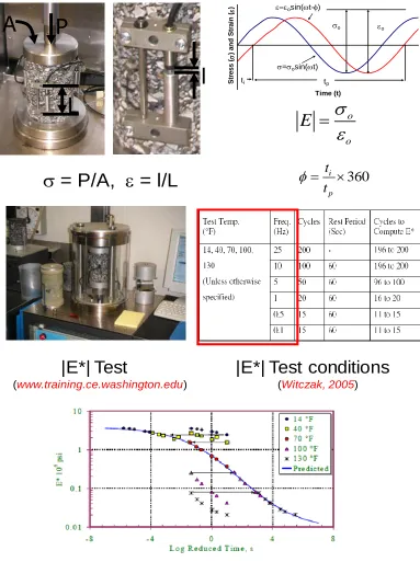
Figure 2. Laboratory AC dynamic modulus (E*) test protocol

P

A

L

l



= P/A,



= l/L

Time (t)

Str

e

s

s

(

)

a

n

d

Str

a

in

(

)

ti

o

=osin(wt)

osin(wt-f)

o

tp

o

o

E







360

i

p t t

f

|E*| Test

(www.training.ce.washington.edu)

|E*| Test conditions

The E* master curves are constructed using frequency-temperature (or time-temperature) superposition concepts represented by shift factors. The combined effects of temperature and loading rate can be represented in the form of a master curve relating E* to a reduced frequency (fr) or a reduced time (tr) by a sigmoidal function. Each of the parameters (i.e., a reduced

frequency [fr] or a reduced time [tr]) utilizes a sigmoidal function equation of the E* master curve. However, the various equations of a sigmoidal function for the E* master curve have been reported in the literature (Pellinen et al. 2004, Schwartz 2005, Witczak 2005, Kutay et al. 2011). For clarification, in this study, the sigmoidal function equation using a reduced frequency (fr) is defined as the dynamic modulus E* master curve equation, while the sigmoidal function equation using a reduced time (tr) is defined as the relaxation modulus E(t) master curve

equation. From the theory of viscoelasticity, E* and E(t) can be converted from each into the other through numerical procedures (Park and Schapery 1999). The dynamic modulus E* master curve equation using a reduced frequency (fr) in this study is described as follows:

3 4

2

1 ( log( ))

*

1 C C fr

C

Log E C

e  

 

 ₍₄₎

Where,

fr= reduced frequency of loading at reference temperature

C1 = minimum value of E*

C1 + C2= maximum value of E*

C3 and C4= parameters describing the shape of the sigmoidal function

The function parameters C1 and C2in general depend on the aggregate gradation and mixture

volumetrics, while the parameters C3and C4 depend primarily on the characteristics of the

asphalt binder (Schwartz 2005). The reduced frequency (fr) can beshown in the following form:

( ) a ( )

r T

f  f T

(5)

Where,

f = frequency of loading at desired temperature T = temperature of interest

aT(T) = shift factor as a function of temperature

The equations widely used to express the temperature-shift factor of aT(T) include

Williams-Landel-Ferry equations, the Arrhenius equations, and the second-order polynomial equations (Pellinen et al. 2004, Witczak 2005, Kutay et al. 2011, Varma et al. 2013b). The shift factor

utilized in this study is the logarithm of the shift factor computed by using a second-order polynomial (Kutay et al. 2011, Varma et al. 2013b), described as follows:

2 2

Where,

Tref= reference temperature, 19C (or 66.2°F)

a1and a2 = the shift factor polynomial coefficients

The values for C1, C2, C3, C4, and aT(T) in a sigmoidal function of master curve are all

simultaneously determined from test data using nonlinear optimization techniques, e.g., the Solver function in Excel software. The relaxation modulus E(t) using a reduced time (tr) can be converted from the dynamic modulus E* using a reduced frequency (fr) through numerical procedures (Park and Schapery 1999) and described as follows:

3 4

2

1 ( log(t ))

( (t))

1 c c r

c

Log E c

e 

 

 ₍₇₎

Where,

tr= reduced time at reference temperature

c1, c2, c3, and c4 = the relaxation modulus E(t) coefficients

FWD Backcalculation

Static FWD Backcalculation Approaches

The FWD backcalculation procedure involves two calculation directions, namely forward and inverse. In the forward direction of analysis, theoretical deflections are computed under the applied load and the given pavement structure using assumed pavement layer moduli. In the inverse direction of analysis, these theoretical deflections are compared with measured deflections, and the assumed moduli are then adjusted in an iterative procedure until the theoretical and measured deflection basins match acceptably well. The moduli derived in this way are considered representative of the pavement response to load and can be used to calculate stresses or strains in the pavement structure for analysis purposes. This is an iterative method of solving the inverse problem and will not have a unique solution in most cases.

Figure 3. Illustration of typical FWD deflection measurements (Goktepe et al. 2006)

Some of the major factors that can lead to erroneous results in backcalculation, and some cautions for avoiding them, are as follows (Irwin 2002, Von Quintus and Killingsworth 1998, Ullidtz and Coetzee 1998):

 There must be a good match between the assumptions that underlie backcalculation and the realities of the pavement.

 The loading is assumed to be static in backcalculation programs while, in reality, FWD loading is dynamic.

 Major cracks in the pavement, or testing near a pavement edge or joint, can cause the deflection data to depart drastically from the assumed conditions.

 Pavements with cracks or various discontinuities and other such features, which are the main focus of maintenance and rehabilitation efforts, are ill-suited for any backcalculation analysis or moduli determination that is based on elastic layered theory.

 FWD deflection data have seating, random, and systematic errors.

 It is seldom clear just how to set up the pavement model. Layer thicknesses are often not known, and subsurface layers can be overlooked. A trial-and-error approach is often used.

 Layer thicknesses are not uniform in the field, nor are materials in the layers completely homogeneous.

 There are vertical changes in the pavement materials and subgrade soils at each site. This change in the vertical profile is minor at some sites, whereas at other sites the change is substantial.

 Some pavement layers are too thin to be backcalculated in the pavement model. Thin layers contribute only a small portion to the overall deflection, and, as a result, the accuracy of their backcalculated values is reduced.

 Moisture contents and depth to hard bottom can vary widely along the road.

 The presence of a shallow water table and related hard layer effects can influence the backcalculation results.

 Most unbound pavement materials are stress-dependent, and most backcalculation programs do not have the capability to handle that.

 Spatial and seasonal variations of pavement layer properties exist in the field.

 Input data effects are a factor. These include seed moduli, modulus limits, and layer thicknesses, as well as program controls such as number of iterations and convergence criteria.

The viscoelastic (VE) pavement properties and dynamic effects such as inertia and damping under FWD testing with dynamic loads can affect the pavement response. However, static backcalculation neglects these effects and therefore less reflects the actual situation. In addition, while the MEPDG uses elastic, plastic, viscous, and creep properties of materials to predict pavement performance over the design life, current static backcalculation methods cannot capture all of these properties. Further, FWD deflection-time history curves contain richer information that have the potential to reduce erroneous results.

Dynamic Backcalculation Approaches

Dynamic pavement response and backcalculation models have been studied by a number of researchers (Al-Khoury et al. 2001a, Al-Khoury et al. 2001b, Al-Khoury et al. 2002a, Al-Khoury et al. 2002b, Callop and Cebon 1996, Chang et al. 1992, Dong et al. 2002, Foinquinos et al. 1995, Goktepe et al. 2006, Grenier and Konrad 2009, Grenier et al. 2009, Hardy and Cebon 1993, Kausel and Roesset 1981, Liang and Zhu 1998, Liang and Zeng 2002, Lytton 1989, Lytton et al. 1993, Magnuson 1998, Magnuson et al. 1991, Maina et al. 2000, Mamlouk and Davies 1984, Mamlouk 1985, Nilsson et al. 1996, Roesset 1980, Roesset and Shao 1985, Shoukry and William 2000, Sousa and Monismith 1987, Stubbs et al. 1994, Ullidtz 2000, Uzan 1994a, Uzan 1994b, Zaghloul and White 1993).

Most of the developed methods employ dynamic pavement response models in the forward calculations of backcalculation procedures. Most of the forward methods adapted analytical or semi-analytical approaches in the solution methodologies, whereas some utilized finite element (FE) or numerical methods.

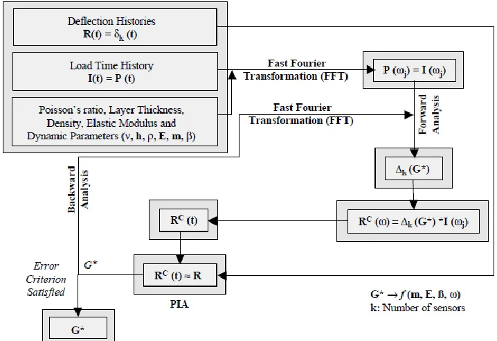
The material properties affecting the dynamic response of a pavement are Young’s modulus (E), complex modulus (G* or E*), Poisson’s ratio (), mass densities (), and damping ratio (). The

present schematic representation of both fitting approaches for dynamic load backcalculation. Fourier analyses and inverse Fourier analyses can be conducted for the transformation of the domain of data.

In frequency domain fitting, the applied load and deflection response time histories are transformed into the frequency domain by using a Fourier transformation. The compliance function of the complex deflection function divided by the complex load function is the measured complex unit response of the pavement at each frequency. Similarly to static

backcalculation methods, an iterative procedure is carried out to find the set of complex moduli that will generate the calculated complex unit response close to the measured one. In time domain fitting, the impulse load time histories should be transformed into the frequency domain data in order to input the available forward model into the frequency domain. Inverse Fourier transformations should be carried out to compare calculated and measured deflections in the time domain.

Some advantages of developed dynamic backcalculation procedures include considering asphalt viscoelastic properties and obtaining more precise results than static procedures. However, some of the limitations of current dynamic backcalculation procedures include the following (Goktepe et al. 2006, Grenier and Konrad 2009):

 The current dynamic backcalculation procedures have more complexity and greater computational expense.

 The error minimization scheme can fall into a local minimum (which may not be the absolute minimum), depending on the complexity of the error function.

 The uniqueness of the solution is not always guaranteed and depends on the number of unknown parameters and the correlation between these parameters.

 Because many observations are used in the dynamic approach, correlations between unknown parameters are usually low, which is not the case in the static approach that uses only the deflection basin.

Viscoelastic Backcalculation Approach

Although many static and dynamic backcalculation approaches have been proposed in the past, only fewer recent studies have attempted to develop dynamic backcalculation approaches to derive the AC E* master curve from FWD defection-time history data.

Kutay et al. (2011) developed a methodology that backcalculates the damaged dynamic modulus

deflection-from a typical FWD test. The study noted that the proposed backcalculation algorithm is

independent of layer geometry because the layer structure and the thickness of the asphalt layer, for the cases analyzed, did not have an influence on the backcalculated E(t) or |E*| master curves. The authors also proposed modifications to the current FWD technology to enable longer FWD pulses and to ensure more reliable readings in the tail regions of the FWD deflection-time histories.

As a follow-up to the work by Kutay et al. (2011), Varma et al. (2013a) estimated and proposed a set of temperatures at which FWD tests should be conducted to be able to maximize the portion of the E(t) curve that can be accurately backcalculated. A genetic algorithm–based (GA-based) viscoelastic backcalculation algorithm was proposed that is capable of predicting E(t) and |E*| master curves as well as time-temperature superposition shift factors from a set of FWD

deflection-time histories at different temperatures. The study concluded that deflection-time

histories from FWD tests conducted between 68–104 °F (20–40 °C) are useful in accurately estimating the entire E(t) or |E*| master curve.

Varma et al. (2013b) considered FWD deflection-time history data from a single FWD drop combined with the temperature gradient across the AC layer at the time of FWD testing in their GA-based viscoelastic backcalculation approach, referred to as BACKLAVA. The study concluded that, unless a stiff layer (bedrock) exists close to the pavement surface that can

DEVELOPMENET OF FRAMEWORK FOR DERIVING AC MASTER CURVE FROM FWD DATA

Based on the research team’s discussions with the Iowa DOT’s Office of Special Investigations and Bituminous Materials Office regarding the specific objectives of this project, the Iowa DOT is eventually interested in documenting the Iowa AC mix damaged master curve coefficients relative to the mix IDs/Station Nos., if possible, in the Pavement Management Information System (PMIS). This would be of significant use to the city, county, and state engineers because the outcome of this research would enable them to look up the damaged master curve shape parameters from the PMIS while running a flexible pavement rehabilitation analysis and design using MEPDG/Pavement ME Design. As a first and foundational step, this feasibility research study focused on establishing frameworks for predicting the AC E(t) master curve coefficients from FWD time history data.

Based on a comprehensive literature review, the existing direct, indirect, and derivative approaches to damaged master curve determination using FWD time history data were synthesized in the previous section. This section describes the development of a detailed framework as a first step in a proof-of-concept demonstration for deriving the AC |E*| master curve coefficients from single-drop FWD time history data.

In the proposed approach, a layered viscoelastic forward analysis tool is first used to generate a database of AC master curve (input)–pavement surface deflection time history (output) scenarios for a variety of pavement layer thicknesses and pavement temperatures (see Figure 6). In the second step, the neural network (NN) methodology is employed to map the AC surface

Figure 6. Schematic of synthetic database development approach using the viscoelastic forward analysis tool

INPUTS

FORWARD ALGORITHM

(Layered Visco-elastic

Program)

• FWD stress-time history

• HMA relaxation modulus curve parameters

• Pavement temperature

• Layer thicknesses

• Poisson's ratios

• Modulus values of base and subgrade

Outputs

Time

(Sec) Deflection (in) at FWD sensors

1 2 3 ……… n

Case#

FORWARD ANALYSIS DATABASE

Case #

1 2 . . . n

Figure 7. Schematic of neural networks approach to predict AC E(t) master curve from FWD deflection-time history data

This simplified approach necessitates the use of a computationally efficient layered VE forward analysis algorithm to generate a database of master curve–dynamic deflection case scenarios for a variety of pavement layer thicknesses and pavement temperatures. The VE forward analysis tool developed by Kutay et al. (2011) was employed for generating the forward synthetic database. This VE forward analysis program attempts to simulate more realistic FWD test conditions with respect to the existence of a nonuniform temperature profile across the depth of the AC layer (Varma et al. 2013a). This enables usage of a single FWD drop to characterize the VE properties, such as time function and time-temperature shifting, to get the AC relaxation modulus master curve, which can subsequently be converted to provide the |E*| master curve.

As mentioned previously, according to the theory of viscoelasticity, if the AC relaxation modulus (E(t)) master curve is known, the AC dynamic modulus (|E*|) master curve can be calculated from it (and vice versa) using well-established numerical inter-conversion procedures (Park and Shapery 1999, Kutay et al. 2011). Since the VE forward analysis program used in this study outputs E(t) master curve parameters, the rest of the analysis and discussion focuses on

Neural Networks Training, Testing and Validation INVERSE MAPPING Inputs • Deflection-time histories [Di[(tj)] • Pavement temperature (tac)

• Pavement layer thicknesses (hac, hb) • Pavement layer

moduli (Eb, Esub) Outputs • HMA relaxation modulus [E(t)] master curve coefficients (c1, c2, c3, and c4) 2 3 n 1 1 1 m 2 p X1 X2 X3 Xn O1 Op T1 Tp Error

Activation process to transport input vector into the network

i

k j

Wij

Q_jk

The backcalculation of shift factors for the master curve requires knowledge of the temperature profile at the time of the FWD testing, which translates into additional dimensions of complexity in the forward analysis and database generation using the current approach. Therefore,

considering the limited project duration and lack of development time, the current approach is restricted to the backcaclulation of AC E(t) master curve coefficients. However, it is

recommended that future research efforts include backcalculation of shift factors for the master curve from FWD deflection-time history data.

Case Studies

First, a preliminary (screening) analysis was carried out for full-depth AC through various case studies to verify the feasibility of the NN approach, identify the promising input features and NN parameters for inverse modeling, and identify associated modeling challenges. The primary goal of these case studies was to answer the question: Are NNs capable of learning/mapping the complex, nonlinear relationship between AC E(t) master curve coefficients and FWD time history data? These case studies (as well as the rest of the report) focus on full-depth AC pavements as a first step to isolate potential backcalculation issues that are only related to the modulus master curve of the AC layer.

Among the several case studies conducted by the research team, three case studies are reported here that systematically varied the inputs for the NN inverse modeling: (1) consider only FWD D0 time history data; (2) consider FWD D0, D8, and D12 time history data; (3) consider only FWD Surface Curvature Index (D0–D12). Here D0, D8, and D12 refer to deflection-time history data recorded at an offset of 0, 8, and 12 inches, respectively, from the center of the FWD

loading plate. It is expected that the effect of viscoelasticity will be more pronounced in the sensors closest to the load plate. Further, some studies have reported that the addition of further sensors in the backcalculation process tends to increase the error in E(t) predictions (Varma et al. 2013a). However, future research should consider all sensors in the standard FWD configuration to elaborately investigate their influence on the accuracy of the backcalculated E(t) master curve and unbound layers.

Development of Synthetic Database

As mentioned previously, the VE forward analysis program outputs pavement surface deflection-time histories based on the following inputs: FWD stress-deflection-time history, AC E(t) master curve coefficients and shift factors, pavement temperature, pavement layer thicknesses and Poisson’s ratios, and unbound layer moduli. The FWD stress-time history for a standard 9 kip loading was used for these case studies and for other analyses discussed in the rest of the report. For full-depth AC analysis, the inputs were reduced to AC E(t) master curve coefficients (c1, c2, c3, and c4) and shift factors (a1 and a2), pavement temperature (Tac), AC layer thickness (Hac), subgrade layer modulus (Esub), AC Poisson’s ratio (μac), and subgrade Poisson’s ratio (μsub).

between the E(t) master curve and deflection-time histories. A synthetic database consisting of 100 scenarios was generated through batch simulations of the VE forward analysis program using the input ranges summarized in Table 1. The min-max ranges of E(t) master curve

coefficients and shift factors are based on the Michigan State University (MSU) E(t) database of 100+ hot-mix asphalt (HMA) mixtures (Varma et al. 2013a).

Table 1. Summary of input ranges used in the generation of 100 VE forward analysis scenarios for case studies

Input Parameter Min Value Max Value

Pavement temperature (Tac) 32 deg-F (0 deg-C) 113 deg-F (45 deg-C)

AC layer thickness (Hac): 20 in. (constant)

Subgrade modulus (Esub): 10,000 psi (constant)

AC Poisson’s ratio (μac): 0.3 (constant)

Subgrade Poisson’s ratio (μsub): 0.4 (constant)

c1 0.045 2.155

c2 1.8 4.4

c3 -0.523 1.025

c4 -0.845 -0.38

a1 -5.380E-4 1.136E-3

a2 -1.598E-1 -0.770E-1

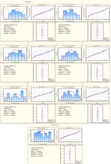
Figure 8. Compound graphs summarizing descriptive statistics, histograms, box plots, and normal probability plots for variable inputs in the synthetic datasets

Tac (deg-C)

K-S d=.10643, p> .20; Lilliefors p<.01 Expected Normal

-10 0 10 20 30 40 50 X <= Category Boundary 0 5 10 15 20 25 30 35 N o . o f o b s.

Mean = 23.146 Mean±SD = (9.9879, 36.3041) Mean±1.96*SD = (-2.6439, 48.9359) -10 0 10 20 30 40 50 60 T a c

Normal P-Plot: T ac

-5 0 5 10 15 20 25 30 35 40 45 50 Value -3 -2 -1 0 1 2 3 E xp e ct e d N o rm a l V a lu e Summary Statistics:Tac Valid N=100 Mean= 23.145975 Minimum= 0.546636 Maximum= 44.774360 Std.Dev.= 13.158101

c1

K-S d=.09698, p> .20; Lilliefors p<.05 Expected Normal

-0.5 0.0 0.5 1.0 1.5 2.0 2.5 X <= Category Boundary 0 5 10 15 20 25 30 35 N o . o f o b s.

Mean = 1.1026 Mean±SD = (0.461, 1.7441) Mean±1.96*SD = (-0.1549, 2.36) -0.4 -0.2 0.0 0.2 0.4 0.6 0.8 1.0 1.2 1.4 1.6 1.8 2.0 2.2 2.4 2.6 c1

Normal P-Plot: c1

-0.2 0.0 0.2 0.4 0.6 0.8 1.0 1.2 1.4 1.6 1.8 2.0 2.2 2.4 Value -3 -2 -1 0 1 2 3 E xp e ct e d N o rm a l V a lu e Summary Statistics:c1 Valid N=100 Mean= 1.102562 Minimum= 0.050683 Maximum= 2.135515 Std.Dev.= 0.641574

c2

K-S d=.11699, p<.15 ; Lilliefors p<.01 Expected Normal

1.5 2.0 2.5 3.0 3.5 4.0 4.5 X <= Category Boundary 0 5 10 15 20 25 30 N o . o f o b s.

Mean = 3.1434 Mean±SD = (2.3696, 3.9172) Mean±1.96*SD = (1.6268, 4.66) 1.5 2.0 2.5 3.0 3.5 4.0 4.5 5.0 c2

Normal P-Plot: c2

1.6 1.8 2.0 2.2 2.4 2.6 2.8 3.0 3.2 3.4 3.6 3.8 4.0 4.2 4.4 4.6 Value -3 -2 -1 0 1 2 3 E xp e ct e d N o rm a l V a lu e Summary Statistics:c2 Valid N=100 Mean= 3.143426 Minimum= 1.821228 Maximum= 4.372656 Std.Dev.= 0.773780

c3

K-S d=.07703, p> .20; Lilliefors p<.15 Expected Normal

-0.8 -0.6 -0.4 -0.20.00.20.40.60.81.01.2 X <= Category Boundary 0 2 4 6 8 10 12 14 16 18 20 22 N o . o f o b s.

Mean = 0.292 Mean±SD = (-0.1391, 0.7231) Mean±1.96*SD = (-0.5529, 1.137) -0.8 -0.6 -0.4 -0.2 0.0 0.2 0.4 0.6 0.8 1.0 1.2 1.4 c3

Normal P-Plot: c3

-0.6 -0.4 -0.2 0.0 0.2 0.4 0.6 0.8 1.0 1.2 Value -3 -2 -1 0 1 2 3 E xp e ct e d N o rm a l V a lu e Summary Statistics:c3 Valid N=100 Mean= 0.292020 Minimum= -0.518842 Maximum= 1.015026 Std.Dev.= 0.431103

c4

K-S d=.12893, p<.10 ; Lilliefors p<.01 Expected Normal

-0.9-0.8 -0.7-0.6-0.5-0.4-0.3-0.2 -0.10.0 X <= Category Boundary 0 5 10 15 20 25 N o . o f o b s.

Mean = -0.4368 Mean±SD = (-0.6906, -0.1829) Mean±1.96*SD = (-0.9343, 0.0607) -1.0 -0.8 -0.6 -0.4 -0.2 0.0 0.2 c4

Normal P-Plot: c4

-0.9 -0.8 -0.7 -0.6 -0.5 -0.4 -0.3 -0.2 -0.1 0.0 Value -3 -2 -1 0 1 2 3 E xp e ct e d N o rm a l V a lu e Summary Statistics:c4 Valid N=100 Mean= -0.436766 Minimum= -0.820522 Maximum= -0.050877 Std.Dev.= 0.253829

a1

K-S d=.11197, p<.20 ; Lilliefors p<.01 Expected Normal

-0.0008

-0.0006-0.0004-0.00020.00000.00020.00040.00060.00080.00100.0012 X <= Category Boundary 0 2 4 6 8 10 12 14 16 18 20 N o . o f o b s.

Mean = 0.0003 Mean±SD = (-0.0002, 0.0008) Mean±1.96*SD = (-0.0007, 0.0013) -0.0008 -0.0006 -0.0004 -0.0002 0.0000 0.0002 0.0004 0.0006 0.0008 0.0010 0.0012 0.0014 0.0016 a1

Normal P-Plot: a1

-0.0006

-0.0004-0.00020.00000.00020.00040.00060.00080.00100.0012 Value -3 -2 -1 0 1 2 3 E xp e ct e d N o rm a l V a lu e Summary Statistics:a1 Valid N=100 Mean= 0.000294 Minimum= -0.000532 Maximum= 0.001093 Std.Dev.= 0.000504

Summary: a2

K-S d=.09302, p> .20; Lilliefors p<.05 Expected Normal

-0.17

-0.16-0.15-0.14-0.13-0.12-0.11-0.10-0.09-0.08-0.07 X <= Category Boundary 0 2 4 6 8 10 12 14 16 18 N o . o f o b s.

Mean = -0.1206 Mean±SD = (-0.1452, -0.096) Mean±1.96*SD = (-0.1688, -0.0724) -0.18 -0.16 -0.14 -0.12 -0.10 -0.08 -0.06 a2

Normal P-Plot: a2

-0.17

The latter portion of the FWD deflection-time history curve typically includes noise and integration errors, and some recent studies have concluded that the current FWD technology needs modification to ensure reliable measurements in the tail regions of the FWD deflection-time histories (Kutay et al. 2011). Consequently, it was decided to use the left half of the deflection-time history data (i.e., up to peak deflections) in the NN inverse modeling. This corresponds to deflection-time histories at the first 20 discrete time intervals, as shown in Figure 9. Box and whisker plots for D0, D8, and D12 deflection-time histories (outputs) are displayed in Figure 10. In these plots, the central square indicates the mean, the box indicates the mean

plus/minus the standard deviation, and whiskers around the box indicate the mean plus/minus 1.96×standard deviation.

Figure 9. Typical deflection-time history generated by the VE forward analysis program at one location. Only the left half of the deflection-time history data was considered in NN

inverse modeling in this study.

Figure 10. Box and whisker plots of D0, D8, and D12 deflection-time histories generated by VE forward analysis simulations for the case studies

t1………..t20

D0 (t1 to t20): Box & Whisker Plot

Mean Mean±SD Mean±1.96*SD D0-1 D0-3 D0-5 D0-7 D0-9 D0-11 D0-13 D0-15 D0-17 D0-19 -0.08 -0.06 -0.04 -0.02 0.00 0.02 0.04 0.06 0.08 0.10 0.12 0.14 0.16

D8 (t1 to t20): Box & Whisker Plot

Mean Mean±SD Mean±1.96*SD D8-1 D8-3 D8-5 D8-7 D8-9 D8-11 D8-13 D8-15 D8-17 D8-19 -0.03 -0.02 -0.01 0.00 0.01 0.02 0.03 0.04 0.05

D12 (t1 to t20): Box & Whisker Plot

traditional methods in civil and transportation engineering applications (Flintsch 2003). They have become standard data fitting tools, especially for problems that are too complex, poorly understood, or resource intensive to tackle using more traditional numerical and/or statistical techniques. They can, in one sense, be viewed as similar to nonlinear regression, except that the functional form of the fitting equation does not need to be specified a priori. The adoption and use of NN modeling techniques in the MEPDG/Pavement-ME Design (NCHRP 2004) has especially placed emphasis on the successful use of neural nets in geomechanical and pavement systems.

Given the successful utilization of NN modeling techniques in the previous IHRB projects focusing on nondestructive evaluation of Iowa pavements and static backcalculation of pavement layer moduli from routine FWD test data (Ceylan et al. 2007, Ceylan et al. 2009, Ceylan et al. 2013), the research team’s first choice was to employ NN for this study. The ability to “learn” the mapping between inputs and outputs is one of the main advantages that make the NNs so attractive. Efficient learning algorithms have been developed and proposed to determine the weights of the network, according to the data of the computational task to be performed. The learning ability of the NNs makes them suitable for unknown and nonlinear problem structures such as pattern recognition, medical diagnosis, time series prediction, and other applications (Haykin 1999).

The NNs in this study were designed, trained, validated, and tested using the MATLAB Neural Network toolbox (Beale et al. 2011). All of the NNs were conventional two-layer (one hidden layer and one output layer) feed-forward networks. Sigmoid transfer functions were used for all hidden layer neurons, while linear transfer functions were employed for the output neurons. Training was accomplished using the Levenberg-Marquardt (LM) backpropagation algorithm. Considerable research has been carried out to accelerate the convergence of learning/training algorithms, which can be broadly classified into two categories: (1) development of ad hoc heuristic techniques that include such ideas as varying the learning rate, using momentum, and rescaling variables; and (2) development of standard numerical optimization techniques.

The three types of numerical optimization techniques commonly used for NN training include the conjugate gradient algorithms, quasi-Newton algorithms, and the LM algorithm. The LM algorithm used in this study is a second-order numerical optimization technique that combines the advantages of Gauss–Newton and steepest descent algorithms. While this method has better convergence properties than the conventional backpropagation method, it requires O(N2) storage and calculations of order O(N2), where N is the total number of weights in a multi-layer

perceptron (MLP) backpropagation. The LM training algorithm is considered to be very efficient when training networks have up to a few hundred weights. Although the computational

requirements are much higher for each iteration of the LM training algorithm, this is more than made up for by the increased efficiency. This is especially true when high precision is required (Beale et al. 2011).

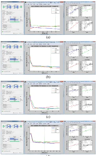
independent testing of the trained model. As mentioned previously, the highlighted case studies considered three input scenarios in the prediction of E(t) master curve coefficients: (1) use only D0 time history data as inputs; (2) use D0, D8, and D12 time history data as inputs; and (3) use only the differences in magnitudes between D0 and D12 time history data (i.e., Surface

(a)

(b)

(c)

(d)

(a)

(b)

(c)

(d)

(a)

(b)

(c)

(d)

Figure 13. NN prediction of E(t) master curve coefficients from differences in magnitudes between D0 and D12 time history data (SCI) using 100 datasets (case study #3): (a) c1, (b)

c2, (c) c3, (d) c4

PROOF-OF-CONCEPT DEMONSTRATION:COMPREHENSIVE FULL-DEPTH AC PAVEMENT ANALYSIS

Development of Comprehensive Synthetic Database

The focused case studies carried out and discussed in the previous section established the framework for deriving the AC E(t) or |E*| master curve based on a single FWD test performed at a single temperature, thereby fulfilling the main objective of this study. In this section, the proposed methodology is further explored through a comprehensive forward and inverse analysis of full-depth AC. A comprehensive synthetic database consisting of 10,000 datasets was

generated through batch simulations of the VE forward analysis program by randomly varying the inputs within the min-max ranges, summarized in Table 2.

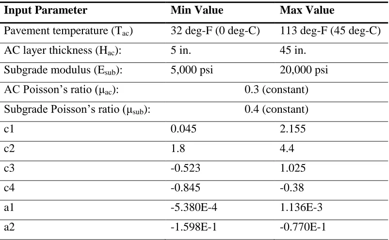
Table 2. Summary of input ranges used in the generation of 10,000 VE forward analysis scenarios for comprehensive full-depth AC analysis

Input Parameter Min Value Max Value

Pavement temperature (Tac) 32 deg-F (0 deg-C) 113 deg-F (45 deg-C)

AC layer thickness (Hac): 5 in. 45 in.

Subgrade modulus (Esub): 5,000 psi 20,000 psi

AC Poisson’s ratio (μac): 0.3 (constant)

Subgrade Poisson’s ratio (μsub): 0.4 (constant)

c1 0.045 2.155

c2 1.8 4.4

c3 -0.523 1.025

c4 -0.845 -0.38

a1 -5.380E-4 1.136E-3

a2 -1.598E-1 -0.770E-1

Graphical comparative summaries (a histogram, box plot, and descriptive statistics) for each of the input variables in the synthetic database are displayed in Figure 14 and Figure 15. The case studies discussed in the previous section tend to indicate that the deflection-time history data at D0, D8, and D12 sensors are necessary inputs for backcalculating the E(t) master curve

Figure 14. Graphical statistical summaries of Tac, Hac, and Esub in the comprehensive raw synthetic database

Graphical Summary(Tac Hac Esub)

Tac -5 0 5 10 15 20 25 30 35 40 45 50 -5 0 5 10 15 20 25 30 35 40 45 50

N: 10000 Mean: 22.46 Median: 22.44 Min: 0.00225 Max: 45.00 L-Qrt: 11.26 U-Qrt: 33.68 Variance: 169 SD: 12.98 Std.Err: 0.130 Skw: 0.00026 Kurt: -1.197

95% Conf SD Lower: 12.80 Upper: 13.16 95% Conf Mean Lower: 22.21 Upper: 22.72

Hac 0 5 10 15 20 25 30 35 40 45 50 0 5 10 15 20 25 30 35 40 45 50

N: 10000 Mean: 25.04 Median: 25.10 Min: 5.003 Max: 45.00 L-Qrt: 15.04 U-Qrt: 35.07 Variance: 134 SD: 11.55 Std.Err: 0.116 Skw: -0.00598 Kurt: -1.199

95% Conf SD Lower: 11.40 Upper: 11.72 95% Conf Mean Lower: 24.82 Upper: 25.27

Esub 2000 4000 6000 8000 10000 12000 14000 16000 18000 20000 22000 2000 4000 6000 8000 10000 12000 14000 16000 18000 20000 22000

N: 10000 Mean: 12523 Median: 12529 Min: 5001 Max: 19999 L-Qrt: 8792 U-Qrt: 16270 Variance: 1.87e+007 SD: 4326 Std.Err: 43.26 Skw: -0.00361 Kurt: -1.197

95% Conf SD Lower: 4266 Upper: 4386 95% Conf Mean Lower: 12438 Upper: 12608

Graphical Summary(c1 c2 c3 c4)

c1 -0.2 0.0 0.2 0.4 0.6 0.8 1.0 1.2 1.4 1.6 1.8 2.0 2.2 2.4 -0.2 0.0 0.2 0.4 0.6 0.8 1.0 1.2 1.4 1.6 1.8 2.0 2.2 2.4

N: 10000 Mean: 1.096 Median: 1.097 Min: 0.0451 Max: 2.155 L-Qrt: 0.566

c2 1.5 2.0 2.5 3.0 3.5 4.0 4.5 5.0 1.5 2.0 2.5 3.0 3.5 4.0 4.5 5.0

N: 10000 Mean: 3.102 Median: 3.106 Min: 1.800 Max: 4.400 L-Qrt: 2.452

c3 -0.8 -0.6 -0.4 -0.2 0.0 0.2 0.4 0.6 0.8 1.0 1.2 -0.8 -0.6 -0.4 -0.2 0.0 0.2 0.4 0.6 0.8 1.0 1.2

N: 10000 Mean: 0.251 Median: 0.251 Min: -0.523 Max: 1.025 L-Qrt: -0.134

c4 -0.9 -0.8 -0.7 -0.6 -0.5 -0.4 -0.3 -0.9 -0.8 -0.7 -0.6 -0.5 -0.4 -0.3

Synthetic Database: Data Pre-processing

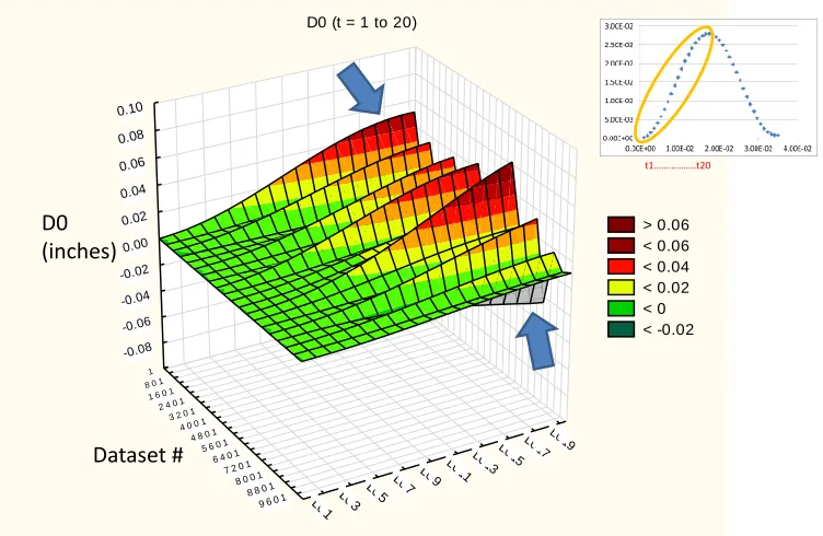
Some anomalies were discovered in the outputs extracted from the results of 10,000 VE forward analysis simulations. It was discovered that the E(t) curves generated by considering the upper and lower limits of c1, c2, c3, and c4 based on the MSU E(t) database of 100+ AC mixtures can result in master curves well outside the database. This can lead to unexpectedly high deflection magnitudes, unreasonable deflection time-histories, and sometimes negative deflections. Some of these anomalies are captured in the D0, D8, and D12 deflection-time histories (outputs) resulting from the 10,000 VE forward runs, depicted in the form of 3-D plots in Figure 16, Figure 17, and Figure 18. To overcome these issues, it was decided to include only those scenarios in the database where the sum of E(t) sigmoid coefficients c1 and c2 was within certain limits. Varma et al. (2013a) used a lower limit of 3.239 and an upper limit of 4.535 based on the MSU database of 100+ AC mixtures. These limits are 4.000 and 5.880, respectively, based on the E(t) curves generated by the ISU research team using the FHWA mobile lab asphalt mixture database.

Figure 16. D0 deflection-time history (from time interval 1 to 20) outputs from 10,000 VE forward analysis simulations

D0 (t = 1 to 20)

1 8 0 1

1 6 01

240 1 3 2 01

4 0 01 4 8 01

5 6 01 6 4 01

7 2 01 8 0 01

8 8 01 9 6 01

D0-1 D0-3

D0-5 D0-7 D0-9

D

0-1₁D0-13D0-15 D0-17D0-19

-0.08 -0.06 -0.04 -0.02 0.00 0.02 0.04

0.06 0.08 0.10

> 0.06 < 0.06 < 0.04 < 0.02 < 0 < -0.02

D0 (inches)

Dataset #

Figure 17. D8 deflection-time history (from time interval 1 to 20) outputs from 10,000 VE forward analysis simulations

D8 (t = 1 to 20)

1 8 0 1 1 6 01

2 4 01 3 2 01

4 0 01 4 8 01

5 6 01

6 4 01 7 2 01

8 0 01 8 8 01

9 6 01 D8

-1 D8-3 D8_-5 D8-7

D8_-9 D8-11D8-13 D8

-15D8-17 D8_-19

-0.08 -0.06 -0.04 -0.02 0.00 0.02 0.04 0.06 0.08 0.10 > 0.04 < 0.04 < 0.03 < 0.02 < 0.01 < 0 D8 (inches) Dataset # t1………..t20

D12 ( t = 1 to 20)

1 8 0 1

1 6 01 2 4 01

3 2 01 4 0 01

4 8 01

5 6 01 6 4 01

7 2 01 8 0 01

8 8 01 9 6 01 D12

-1 D12-3

D12_-5 D12-7 D12-9

D12_-11D12-13D12-15 D12_-17D12-1₉

-0.08 -0.06 -0.04 -0.02 0.00

0.02

3,338. Graphical comparative summaries for each of the input variables in the processed synthetic database are displayed in Figure 19 and Figure 20. The D0, D8, and D12 deflection-time histories (outputs) from the processed synthetic database captured in Figure 21, Figure 22, and Figure 23 appear reasonable.

Figure 19. Graphical statistical summaries of Tac, Hac, and Esub in the processed synthetic database

Figure 20. Graphical statistical summaries of c1, c2, c3, and c4 in the processed synthetic

Graphical Summary(Tac Hac Esub)

Tac -5 0 5 10 15 20 25 30 35 40 45 50 -5 0 5 10 15 20 25 30 35 40 45 50

N: 3338 Mean: 18.90 Median: 17.54 Min: 0.00715 Max: 45.00 L-Qrt: 8.806 U-Qrt: 28.20 Variance: 145 SD: 12.03 Std.Err: 0.208 Skw: 0.320 Kurt: -0.934 95% Conf SD Lower: 11.75 Upper: 12.33 95% Conf Mean Lower: 18.49 Upper: 19.30

Hac 0 5 10 15 20 25 30 35 40 45 50 0 5 10 15 20 25 30 35 40 45 50

N: 3338 Mean: 26.95 Median: 27.43 Min: 5.010 Max: 44.99 L-Qrt: 18.04 U-Qrt: 36.28 Variance: 116 SD: 10.76 Std.Err: 0.186 Skw: -0.126 Kurt: -1.100 95% Conf SD Lower: 10.51 Upper: 11.03 95% Conf Mean Lower: 26.59 Upper: 27.32

Esub 2000 4000 6000 8000 10000 12000 14000 16000 18000 20000 22000 2000 4000 6000 8000 10000 12000 14000 16000 18000 20000 22000

N: 3338 Mean: 12839 Median: 12992 Min: 5002 Max: 19999 L-Qrt: 9212 U-Qrt: 16532 Variance: 1.84e+007 SD: 4291 Std.Err: 74.27 Skw: -0.0890 Kurt: -1.175 95% Conf SD Lower: 4191 Upper: 4397 95% Conf Mean Lower: 12693 Upper: 12984

Graphical Summary(c1 c2 c3 c4)

c1 -0.2 0.0 0.2 0.4 0.6 0.8 1.0 1.2 1.4 1.6 1.8 2.0 2.2 2.4 -0.2 0.0 0.2 0.4 0.6 0.8 1.0 1.2 1.4 1.6 1.8 2.0 2.2 2.4

N: 3338 Mean: 1.072 Median: 1.083 Min: 0.0461 Max: 2.152 L-Qrt: 0.579 U-Qrt: 1.542 Variance: 0.335 SD: 0.578 Std.Err: 0.0100 Skw: 0.00167 Kurt: -1.112 95% Conf SD Lower: 0.565

c2 1.5 2.0 2.5 3.0 3.5 4.0 4.5 5.0 1.5 2.0 2.5 3.0 3.5 4.0 4.5 5.0

N: 3338 Mean: 2.881 Median: 2.840 Min: 1.800 Max: 4.389 L-Qrt: 2.370 U-Qrt: 3.332 Variance: 0.384 SD: 0.620 Std.Err: 0.0107 Skw: 0.256 Kurt: -0.837 95% Conf SD Lower: 0.605

c3 -0.8 -0.6 -0.4 -0.2 0.0 0.2 0.4 0.6 0.8 1.0 1.2 -0.8 -0.6 -0.4 -0.2 0.0 0.2 0.4 0.6 0.8 1.0 1.2

N: 3338 Mean: 0.320 Median: 0.349 Min: -0.523 Max: 1.025 L-Qrt: -0.0485 U-Qrt: 0.701 Variance: 0.191 SD: 0.437 Std.Err: 0.00757 Skw: -0.170 Kurt: -1.143 95% Conf SD Lower: 0.427

c4 -0.9 -0.8 -0.7 -0.6 -0.5 -0.4 -0.3 -0.9 -0.8 -0.7 -0.6 -0.5 -0.4 -0.3

Figure 21. D0 deflection-time history (from time interval 1 to 20) outputs in the processed synthetic database

Figure 22. D8 deflection-time history (from time interval 1 to 20) outputs in the processed synthetic database

D0 ( t = 1 to 20)

1 269₅₃7

805 1073₁₃41

1609₁₈77

2145₂₄13 2681₂₉49

3217 D 0 -1 D 0 -3D 0 -5

D 0 -7D 0 -9 D 0 -11D 0 -13

D 0 -15 D 0 -17

D 0 -19

0.000 0.002 0.004 0.006 0.008 0.010 0.012 0.014 0.016 0.018 0.020

0.022

0.024 0.026 D0 (inches) Dataset # t1………..t20

D8 ( t= 1 to 20)

1 269 537 805 1073 1341 1609 1877 2145 2413 2681 2949

3217 D8-1 D8-3D8-5

D8-7D8-9 D8-11

Figure 23. D12 deflection-time history (from time interval 1 to 20) outputs in the processed synthetic database

Neural Networks Forward Modeling

Before carrying out NN inverse modeling to map E(t) master curve coefficients from FWD deflection-time histories, NN forward modeling was carried out to see how accurately NNs can predict the individual deflection-time histories (D0, D8, and D12) based on NN E(t) master curve coefficients and other inputs in the processed synthetic database. If successful, the NN forward model could also serve as a surrogate model (within the specified input ranges) that could replace the VE forward analysis runs.

Based on a parametric sensitivity analysis, a conventional two-layer (1 hidden layer with 25 neurons and 1 output layer) feed-forward network was deemed sufficient for forward modeling. Sigmoid transfer functions were used for all hidden layer neurons, while linear transfer functions were employed for the output neurons. Training was accomplished using the LM

backpropagation algorithm implemented in the MATLAB NN Toolbox. Separate NN models were developed for each of the deflections (3 sensor locations and 20 time intervals). Thus, the model inputs were E(t) master curve coefficients (c1, c2, c3, and c4), Tac, Hac, and Esub. Seventy percent of the 3,338 datasets were used for training, 15% were used for validation (to halt training when generalization stops improving), and 15% were used for independent testing of the trained model.

The NN forward modeling regression results for predicting D0, D8, and D12 deflection-time histories are summarized in Figure 24, Figure 25, and Figure 26, respectively. As seen in these plots, except for the first two or three time intervals, deflection-time histories at all other time intervals are predicted by NN analysis with very high accuracy (R-values greater than 0.97).

D12 ( t = 1 to 20)

1 2 6 9

5 3 7 8 0 5

1 0 73 1 3 41

1 6 09 1 8 77

2 1 45

241 3

2 6 81 2 9 49

3 2 17 D12_-1D12-3

D12_-5D12-7D12-9 D12_-11D12-13D12-15

D12_-17D12-19 0.000

0.002 0.004 0.006 0.008 0.010

0.012 0.014 0.016 0.018 0.020 0.022 0.024

D12 (inches)

Dataset #

Figure 24. NN forward modeling regression results for predicting D0 deflection-time history data from E(t) master curve coefficients

Figure 25. NN forward modeling regression results for predicting D8 deflection-time history data from E(t) master curve coefficients

D0-1 D0-2 D0-3 D0-4 D0-5 D0-6 D0-7

D0-8 D0-9 D0-10 D0-11 D0-12 D0-13 D0-14

D0-15 D0-16 D0-17 D0-18 D0-19 D0-20

D8-1 D8-2 D8-3 D8-4 D8-5 D8-6 D8-7

D8-8 D8-9 D8-10 D8-11 D8-12 D8-13 D8-14

Figure 26. NN forward modeling regression results for predicting D12 deflection-time history data from E(t) master curve coefficients

Neural Networks Inverse Modeling Considering only D0, D8, and D12

The processed synthetic database consisting of 3,338 input-output scenarios was utilized in developing NN inverse models for predicting E(t) master curve coefficients from FWD

deflection-time histories by considering only D0, D8, and D12 sensors. The inputs, outputs, and the generic network architecture details for the NN inverse mapping models are summarized in Figure 27.

D12-1 D12-2 D12-3 D12-4 D12-5 D12-6 D12-7

D12-8 D12-9 D12-10 D12-11 D12-12 D12-13 D12-14

D12-15 D12-16 D12-17 D12-18 D12-19 D12-20

Inputs

• D0, D8, D12

Deflection-time histories [D0(tj)] (j = 4 to 20)

• Tac

• Hac

• Esub

Outputs

• HMA relaxation

modulus [E(t)] master curve coefficients (c1, c2, c3, and c4)

3 4

2 1 ( log(t ))

( (t))

1 c c r

c

Log E c

e 

  

Generic network architecture: 54-h-1

54inputs: Tac, Hac, Esub, D0(tj); D8(tj);D12(tj)[j= 4 to 20]

hhidden neurons