Development of a Computational Framework for Big Data-Driven Prediction of Long-Term Bridge Performance and Traffic Flow

InTrans Project Reports Institute for Transportation

4-2018

Development of a Computational Framework for

Big Data-Driven Prediction of Long-Term Bridge

Performance and Traffic Flow

In Ho Cho

Iowa State University, [email protected]

An Chen

Iowa State University, [email protected]

Alice Alipour

Iowa State University, [email protected]

Behrouz Shafei

Iowa State University, [email protected]

Simon Laflamme

Iowa State University, [email protected]

See next page for additional authors

Follow this and additional works at:https://lib.dr.iastate.edu/intrans_reports

Part of theCivil Engineering Commons,Construction Engineering and Management Commons, and theTransportation Engineering Commons

Recommended Citation

Cho, In Ho; Chen, An; Alipour, Alice; Shafei, Behrouz; Laflamme, Simon; Song, Ikkyun; and Yan, Jin, "Development of a Computational Framework for Big Data-Driven Prediction of Long-Term Bridge Performance and Traffic Flow" (2018).InTrans Project Reports. 223.

Development of a Computational Framework for Big Data-Driven

Prediction of Long-Term Bridge Performance and Traffic Flow

Abstract

Consistent efforts with dense sensor deployment and data gathering processes for bridge big data have accumulated profound information regarding bridge performance, associated environments, and traffic flows. However, direct applications of bridge big data to long-term decision-making processes are hampered by big data-related challenges, including the immense size and volume of datasets, too many variables, heterogeneous data types, and, most importantly, missing data. The objective of this project was to develop a foundational computational framework that can facilitate data collection, data squashing, data merging, data curing, and, ultimately, data prediction. By using the framework, practitioners and researchers can learn from past data, predict various information regarding long-term bridge performance, and conduct data-driven efficient planning for bridge management and improvement. This research project developed and validated several computational tools for the aforementioned objectives. The programs include (1) a data-squashing tool that can shrink years-long bridge strain sensor data to manageable datasets, (2) a data-merging tool that can synchronize bridge strain sensor data and traffic flow sensor data, (3) a data-curing framework that can fill in arbitrarily missing data with statistically reliable values, and (4) a data-prediction tool that can accurately predict bridge and traffic data. In tandem, this project performed a foundational investigation into dense surface sensors, which will serve as a new data source in the near future. The resultant hybrid datasets, detailed manuals, and examples of all programs have been developed and are shared via web folders. The conclusion from this research was that the developed framework will serve practitioners and researchers as a powerful tool for making big data-driven predictions regarding the long-term behavior of bridges and relevant traffic information.

Keywords

bridge big data, bridge data prediction, data merging, data squashing, missing data curing, traffic data prediction

Disciplines

Civil Engineering | Construction Engineering and Management | Transportation Engineering

Comments

Visit www.intrans.iastate.edu for color pdfs of this and other research reports.

Authors

In Ho Cho, An Chen, Alice Alipour, Behrouz Shafei, Simon Laflamme, Ikkyun Song, and Jin Yan

Development of a Computational

Framework for Big Data-Driven

Prediction of Long-Term Bridge

Performance and Traffic Flow

Final Report

April 2018

Sponsored by

About MTC

The Midwest Transportation Center (MTC) is a regional University Transportation Center (UTC) sponsored by the U.S. Department of Transportation Office of the Assistant Secretary for Research and Technology (USDOT/OST-R). The mission of the UTC program is to advance U.S. technology and expertise in the many disciplines comprising transportation through the mechanisms of education, research, and technology transfer at university-based centers of excellence. Iowa State University, through its Institute for Transportation (InTrans), is the MTC lead institution.

About InTrans

The mission of the Institute for Transportation (InTrans) at Iowa State University is to develop and implement innovative methods, materials, and technologies for improving transportation efficiency, safety, reliability, and sustainability while improving the learning environment of students, faculty, and staff in transportation-related fields.

ISU Non-Discrimination Statement

Iowa State University does not discriminate on the basis of race, color, age, ethnicity, religion, national origin, pregnancy, sexual orientation, gender identity, genetic information, sex, marital status, disability, or status as a U.S. veteran. Inquiries regarding non-discrimination policies may be directed to Office of Equal Opportunity, 3410 Beardshear Hall, 515 Morrill Road, Ames, Iowa 50011, Tel. 515-294-7612, Hotline: 515-294-1222, email [email protected].

Notice

The contents of this report reflect the views of the authors, who are responsible for the facts and the accuracy of the information presented herein. The opinions, findings and conclusions expressed in this publication are those of the authors and not necessarily those of the sponsors. This document is disseminated under the sponsorship of the U.S. DOT UTC program in the interest of information exchange. The U.S. Government assumes no liability for the use of the information contained in this document. This report does not constitute a standard, specification, or regulation.

The U.S. Government does not endorse products or manufacturers. If trademarks or

manufacturers’ names appear in this report, it is only because they are considered essential to the objective of the document.

Quality Assurance Statement

Technical Report Documentation Page

1. Report No. 2. Government Accession No. 3. Recipient’s Catalog No.

4. Title and Subtitle 5. Report Date

Development of a Computational Framework for Big Data-Driven Prediction of Long-Term Bridge Performance and Traffic Flow

April 2018

6. Performing Organization Code

7. Author(s) 8. Performing Organization Report No.

In Ho Cho, An Chen, Alice Alipour, Behrouz Shafei, Simon Laflamme, Ikkyun Song, and Jin Yan

9. Performing Organization Name and Address 10. Work Unit No. (TRAIS)

Institute for Transportation Iowa State University

2711 South Loop Drive, Suite 4700 Ames, IA 50010-8664

11. Contract or Grant No.

Part of DTRT13-G-UTC37

12. Sponsoring Organization Name and Address 13. Type of Report and Period Covered Midwest Transportation Center

2711 S. Loop Drive, Suite 4700 Ames, IA 50010-8664

U.S. Department of Transportation Office of the Assistant Secretary for Research and Technology

1200 New Jersey Avenue, SE Washington, DC 20590

Final Report

14. Sponsoring Agency Code

15. Supplementary Notes

Visit www.intrans.iastate.edu for color pdfs of this and other research reports. 16. Abstract

Consistent efforts with dense sensor deployment and data gathering processes for bridge big data have accumulated profound information regarding bridge performance, associated environments, and traffic flows. However, direct applications of bridge big data to long-term decision-making processes are hampered by big data-related challenges, including the immense size and volume of datasets, too many variables, heterogeneous data types, and, most importantly, missing data. The objective of this project was to develop a foundational computational framework that can facilitate data collection, data squashing, data merging, data curing, and, ultimately, data prediction. By using the framework, practitioners and researchers can learn from past data, predict various information regarding long-term bridge performance, and conduct data-driven efficient planning for bridge management and improvement.

This research project developed and validated several computational tools for the aforementioned objectives. The programs include (1) a data-squashing tool that can shrink years-long bridge strain sensor data to manageable datasets, (2) a data-merging tool that can synchronize bridge strain sensor data and traffic flow sensor data, (3) a data-curing framework that can fill in arbitrarily missing data with statistically reliable values, and (4) a data-prediction tool that can accurately predict bridge and traffic data. In tandem, this project performed a foundational investigation into dense surface sensors, which will serve as a new data source in the near future. The resultant hybrid datasets, detailed manuals, and examples of all programs have been developed and are shared via web folders.

The conclusion from this research was that the developed framework will serve practitioners and researchers as a powerful tool for making big data-driven predictions regarding the long-term behavior of bridges and relevant traffic information.

17. Key Words 18. Distribution Statement

bridge big data—bridge data prediction—data merging—data squashing— missing data curing—traffic data prediction

No restrictions.

19. Security Classification (of this report)

20. Security Classification (of this page)

21. No. of Pages 22. Price

Unclassified. Unclassified. 48 NA

D

EVELOPMENT OF A

C

OMPUTATIONAL

F

RAMEWORK FOR

B

IG

D

ATA

-D

RIVEN

P

REDICTION

OF

L

ONG

-T

ERM

B

RIDGE

P

ERFORMANCE AND

T

RAFFIC

F

LOW

Final Report April 2018

Principal Investigator

In Ho Cho, Assistant Professor

Civil, Construction, and Environmental Engineering, Iowa State University

Co-Principal Investigators

An Chen, Assistant Professor

Civil, Construction, and Environmental Engineering, Iowa State University Alice Alipour, Structure and Infrastructure Engineer

Institute for Transportation, Iowa State University Behrouz Shafei, Structural Engineer Bridge Engineering Center, Iowa State University

Investigators

Simon Laflamme, Associate Professor

Civil, Construction, and Environmental Engineering, Iowa State University Brent Phares, Director

Bridge Engineering Center, Iowa State University

Authors

In Ho Cho, An Chen, Alice Alipour, Behrouz Shafei, Simon Laflamme, Ikkyun Song, and Jin Yan

Sponsored by

Midwest Transportation Center and U.S. Department of Transportation

Office of the Assistant Secretary for Research and Technology

A report from

Institute for Transportation Iowa State University

TABLE OF CONTENTS

ACKNOWLEDGMENTS ... IX

EXECUTIVE SUMMARY ... XI

1 INTRODUCTION ...1

1.1 Problem Statement ...1

1.2 Research Approach and Methods ...1

2 LITERATURE REVIEW ...4

3 DATA COLLECTION FROM A TARGET BRIDGE ...5

4 DATA SQUASHING ...6

5 DATA MERGING WITH TRAFFIC FLOW DATA ...9

6 DATA CURING ...10

7 DATA PREDICTION ...11

7.1 Theoretical Summary of GAM ...11

7.2 Direct Search Method for the Best Predictive Power ...12

7.3 Prediction of Traffic Flow Data ...20

8 VARIOUS IMPACTS ON DATA PREDICTION ...22

8.1 Impact of Data Curing on Data Prediction ...22

8.2 Impact of Inclusion of Traffic Data on the Prediction of Bridge Data ...22

9 INVESTIGATION INTO NEW DATA SOURCE – SURFACE SENSORS ...24

9.1 Background on Surface Sensors ...24

9.2 Surface Sensor Fabrication ...25

9.3 Experiment Setup and Instrumentation of Surface Sensor ...26

9.4 Results and Discussion of Surface Sensor Tests...27

10 DOWNLOADABLE PROGRAMS AND DATA ...32

10.1 Data Processing Programs ...32

10.2 Final Datasets ...32

11 CONCLUSIONS...33

vi

LIST OF FIGURES

Figure 1. Computational job distribution in the high-performance computing facility ...3 Figure 2. Instrumentation plan of sensors on the target bridge on eastbound I-80 over Sugar

Creek ...5 Figure 3. Flow chart showing data squashing, data transferring, and data merging of bridge

sensor data and traffic flow data ...6 Figure 4. Strain history over 10 minutes (left) and in a 1-minute time frame (right), with

top and bottom peaks outside the range of +5µ and -5 µ from the median strain

value selected ...7 Figure 5. Example of the total counts of relative peak strains in different bins ...8 Figure 6. Example of a resultant dataset after merging bridge sensor data and traffic sensor

data ...9 Figure 7. Comparison of prediction performance between GAM and other methods (i.e.,

multiple linear regression, SVM, and ERT)...12 Figure 8. Comparison of prediction errors generated by direct search method and

correlation-based selection ...17 Figure 9. Variation of prediction errors with different combination of predictors during

traffic flow data prediction ...20 Figure 10. Quantile-quantile (Q-Q) plots of the original traffic data and the predicted traffic

data: (a) small vehicles (R2 _{= 0.77), (b) medium vehicles (R}2 _{= 0.44), (c) large}

vehicles (R2 = 0.70) ...21 Figure 11. Comparison of prediction performance of GAM when using bridge big data

after data curing by imputation (blue-colored bars) and before data curing, i.e.,

with missing data (orange-colored bars) ...22 Figure 12. Comparison of prediction performance of GAM when using bridge big data

after merging with traffic data (blue-colored bars) and without traffic data

(orange-colored bars) ...23 Figure 13. Sensor fabrication process ...26 Figure 14. Experimental setup of surface sensor, from left to right, front view, side view,

and MTS setup ...26 Figure 15. Surface sensor test results for force and stress versus strain curves ...28 Figure 16. Surface sensor test results showing the failure modes of the specimens, from left

LIST OF TABLES

Table 1. Summary of datasets generated from the raw bridge and traffic big data ...8

Table 2. Summary of predictor (explanatory) and response (target) variables used for the statistical prediction model ...14

Table 3. Correlations among all variables of bridge and traffic big data ...16

Table 4. Best combinations of predictors selected by the direct search method ...19

Table 5. Mechanical properties of CFRP components provided from the supplier ...25

Table 6. Specimen configuration ...27

ACKNOWLEDGMENTS

The investigators would like to express sincere gratitude to the Institute for Transportation’s Midwest Transportation Center at Iowa State University and the U.S. Department of

EXECUTIVE SUMMARY

Damage on state bridges results from various structural and environmental factors, traffic flows, and the complex interactions among these factors. Predicting long-term performance and

determining strategies for the cost-effective management of bridges have been formidable

challenges. By virtue of advanced sensing technologies, various real-time high-precision data for bridges are becoming available. Immense information available from the new data on bridges (dubbed “bridge big data” herein) is believed to improve the predictive accuracy of long-term bridge performance. Consistent efforts with dense sensor deployment and data gathering processes for bridge big data have accumulated profound information regarding bridge

performance, associated environments, and traffic flows. However, direct applications of bridge big data to long-term decision-making processes are hampered by big data-related challenges, including the immense size and volume of datasets, too many variables, heterogeneous data types, and, most importantly, missing data.

The objective of this project was to develop a foundational computational framework that can facilitate data collection, data squashing, data merging, data curing, and data prediction. By using the framework, practitioners and researchers can learn from past data, predict various

information regarding long-term bridge performance, and conduct data-driven efficient planning for bridge management and improvement.

This research project developed and validated several computational tools for the

aforementioned objectives. The programs include (1) a data-squashing tool that can shrink years-long bridge strain sensor data to manageable datasets, (2) a data-merging tool that can

synchronize bridge strain sensor data and traffic sensor data, (3) a data-curing framework that can fill in arbitrarily missing data with statistically reliable values, and (4) a data-prediction tool that can accurately predict bridge behavior as well as traffic flow data. Detailed manuals and examples for all programs have been developed and are shared, and resultant hybrid bridge data are provided. In tandem, this project also performed investigations into a new data source of surface sensors. Understanding the new refined data source of surface sensors is important for a general extension of the developed framework.

1 INTRODUCTION

1.1 Problem Statement

To effectively manage over 600,000 bridges nationwide, the bridge structural health monitoring (SHM) field has made remarkable advancements. To date, advances in bridge SHM have provided an immense amount of bridge data, such as years-long strain and temperature data. Still, engineers and stakeholders lack substantially reliable data analysis and processing tools that have statistical rigor. This project sought to transform the management and analysis of big data as used to understand bridge performance and thereby proposes new data-driven remedies to long-term infrastructure management and rehabilitation. The data-driven paradigm shift will eventually lead to substantial cost savings in bridge management in Iowa and beyond.

However, direct applications of bridge big data and traffic big data to long-term decision-making processes are critically hampered by big data-related challenges. The key aspects of the

challenges include the immense size and volume of datasets for bridge and traffic big data, too many explanatory variables (also called “predictors”) that are complicatedly interwoven, heterogeneous types of bridges, time-varying environmental data and traffic datasets, and, most importantly, the critical issue of missing data in bridge big data.

The objective of this project was to develop a foundational computational framework that can facilitate data collection, data squashing, data merging, data curing, and, ultimately, data prediction. By using the framework, practitioners and researchers can learn from past data, predict information that is pertinent to long-term bridge performance, and conduct data-driven efficient planning for bridge management and improvement.

This research project developed and validated several computational tools for the

aforementioned objectives. The programs include (1) a data-squashing tool that can shrink years-long bridge strain sensor data to manageable datasets, (2) a data-merging tool that can

synchronize bridge strain sensor data and traffic sensor data, (3) a data-curing framework that can fill in arbitrarily missing data with statistically reliable values, and (4) a data-prediction tool that can accurately predict bridge and traffic data. In tandem, this project performed an

investigation into the new data source of dense surface sensors. Detailed manuals and examples for all programs have been developed and are shared, and resultant hybrid bridge data are provided.

1.2 Research Approach and Methods

2

1.2.1 Task 1: Efficient Data Squashing

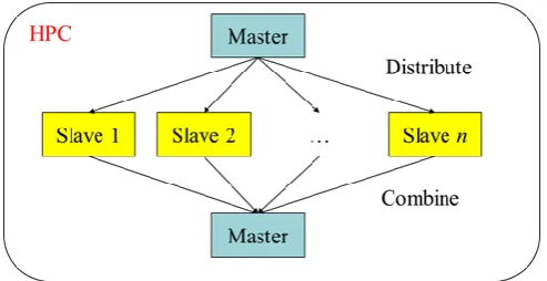
This project developed a computational tool that runs on the high-performance computing (HPC) facility (named the Condo cluster) of the College of Engineering at Iowa State University. For data merging between bridge sensor data and traffic sensor data, this project developed a computational tool that automatically synchronizes the two disparate databases.

1.2.2 Task 2: Missing Data Curing

One of the advanced statistical imputation methods, fractional hot deck imputation (FHDI), was adopted to cure the missing values in the bridge sensor data. The data curing was conducted prior to building a statistical prediction model.

1.2.3 Task 3: Data Prediction

An advanced statistical method, the generalized additive model (GAM) developed by Hastie and Tibshirani (1990), has been adopted and modified for this project. Compared to other machine learning (ML) algorithms, GAM proved to be a general and powerful predictive model for strain values of the target bridge, as well as associated traffic flows. As will be addressed later in this report, GAM is a nonparametric statistical model that is flexible and has little restriction to a large number of predictors (i.e., GAM allows many variables to serve as predictor variables). Importantly, not all variables are necessary in the prediction model to achieve the highest

prediction accuracy. Rather than simply use a correlation-based selection of important variables, this project developed a direct search method to find the best combination of predictors that can lead to the highest prediction accuracy.

1.2.4 Task 4: Understanding New Surface Sensors

A systematic experimental approach was used to better understand the new data source of dense surface sensors.

1.2.5 Task 5: High-Performance Computing (HPC)

Figure 1. Computational job distribution in the high-performance computing facility

4

2 LITERATURE REVIEW

Data-driven research recently has been essential in the engineering field and has enabled researchers to gain valuable knowledge from data analysis. Recently, researchers have focused on a novel combination of advanced machine learning methods and existing engineering databases. For instance, Lv et al. (2015) developed a traffic flow model using the deep learning method. Perera and Mo (2016) utilized a deep learning algorithm to generate a condensed database regarding ship performance and navigation information for general use in the relevant research. Le and Jeong (2017) developed a methodology to integrate heterogeneous

terminologies, which are equivalent, into representative terms by using a neural network. These studies have shown the promising capabilities of automated data accumulation processes.

Meanwhile, due to advances in strain measurement technologies, bridge health monitoring (BHM) systems using various types of sensors have become available. Good examples can be found in the works of Jang et al. (2010), Ko and Ni (2005), Li et al. (2004), and Ntotsios et al. (2009). Such BHM technologies have contributed to the size, volume, and velocity (i.e., the degree of data size increase) of data. Despite such advances in bridge strain databases, the cumulated data have rarely been used to build a prediction model that can help forecast long-term bridge performance and thus improve the management planning of bridges. Earlier works utilized typical statistical methods. For instance, Li et al. (2003) developed a statistical model to represent a specific daily cycle of bridge data using multiple linear regression (MLR). Yet, the simplicity of their statistical model posed challenges to a general application. The daily strain history pattern and the size of a pulse do not remain constant over time and may be affected by many other intractable factors, such as temperature and traffic.

3 DATA COLLECTION FROM A TARGET BRIDGE

The target bridge is located on eastbound I-80 over Sugar Creek in Iowa. Seventy-one sensors were installed in multiple locations of the bridge to measure strains in the top and bottom flanges and to measure the temperatures of the steel, concrete, and air. Fifty-three sensors were installed at the bottom flanges and others were installed at the top flanges. The detailed instrumental plan is shown in Figure 2.

Figure 2. Instrumentation plan of sensors on the target bridge on eastbound I-80 over Sugar Creek

Each sensor measures temperature and strain data at its location at a frequency of 250 Hz. The data have been collected since June 2016. A raw data file spans a 1-minute time frame and contains various information, including date, time, temperature, and the strains measured by a total of 71 sensors. The raw data need to be converted to an interpretable form within a dataset for subsequent data analysis and prediction. The procedure for the extraction and transformation of data is described in the following chapters.

6

4 DATA SQUASHING

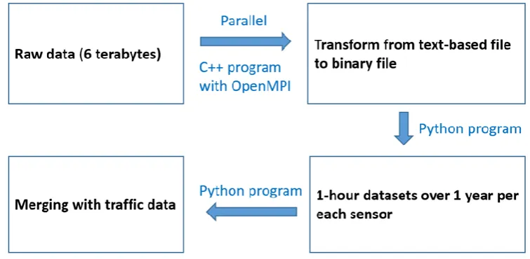
For efficient data learning, analysis, and prediction, some salient information needed to be extracted from the raw data files and transformed into a compact and manageable size. Due to the huge size of the dataset (i.e., about six terabytes), it was infeasible to manipulate the raw data using a single workstation because it would take too much time for a few central processing units (CPUs) to extract and transform the data. Therefore, the entire set of raw data was transferred to the HPC cluster, and the raw data were transformed to an interpretable and manageable form (e.g., several megabytes). The data-squashing workflow of these procedures is shown in Figure 3.

Figure 3. Flow chart showing data squashing, data transferring, and data merging of bridge sensor data and traffic flow data

Figure 4. Strain history over 10 minutes (left) and in a 1-minute time frame (right), with top and bottom peaks outside the range of +5µ and -5 µ from the median strain value

selected

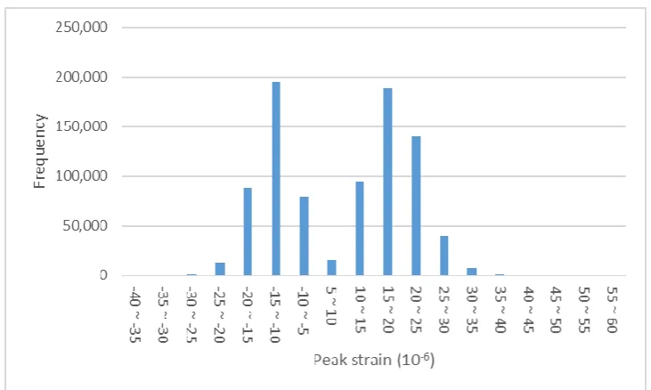
The top and bottom peak strains are determined in such a way that their absolute values are greater than 5µ (here, µ = 10-6) from the median strain value. The median strain is calculated from the strains within the 1-minute time frame. Small peak strains near the median value of strains (i.e., strains for which the distance from the median is less than 5µ strain) are considered to be noise.

It should be noted that all the peaks are of “relative” strains measured from the median strain within the 1-minute time frame. Since the relative strain is linked with external force-induced bridge deformations, this project focused on relative strains throughout the project.

Next, the binary files are transformed to a 1-hour dataset in which one instance, (i.e., one row) consists of a number of information columns. Starting from the leftmost column, each column includes the following information:

 8 digits (e.g., 20161115) representing the year, month, and day

 Hour (i.e., 0 through 24 hours)

 Day of week (i.e., 1 through 7, where 2 means Tuesday, 3 means Wednesday, and so on)

 Steel temperature

 Concrete temperature

 Air temperature

 Median strain in 1-minute time frame

 Number of measurements

 Frequencies of peak strain

 Sensor location in (x,y,z) coordinates

 Sensor index

8

Figure 5. Example of the total counts of relative peak strains in different bins

The summary of datasets created by the transformation step is presented in Table 1. After data squashing/merging, the size of the data set becomes smaller than that of the original.

Table 1. Summary of datasets generated from the raw bridge and traffic big data

Dataset name

(data format) Size Attribute Description

Raw data

(text-based format) < 10 TB Date, time, temperature, strain

Raw data measured with 250 Hz by sensor installed in the bridge

Binary data (binary

format) 100 MB

Date, time, average temperature, peak strain, number of measurements

A single instance contains information for 1 minute

1-hour dataset (csv

format) 10 MB

Date, time, day of week, average temperature, number of measurements and median of strain over 1 hour, strain frequencies

A single instance contains information for 1 hour

1-hour dataset with

traffic (csv format) 10 MB

Date, time, day of week, average temperature, number of measurements and median of strain over 1 hour, strain frequencies, traffic

5 DATA MERGING WITH TRAFFIC FLOW DATA

Traffic is believed to directly affect the behavior of bridges. Heavy traffic generates considerably broad strain fluctuations, and thus the passing of heavy vehicles (e.g., heavy trucks) may

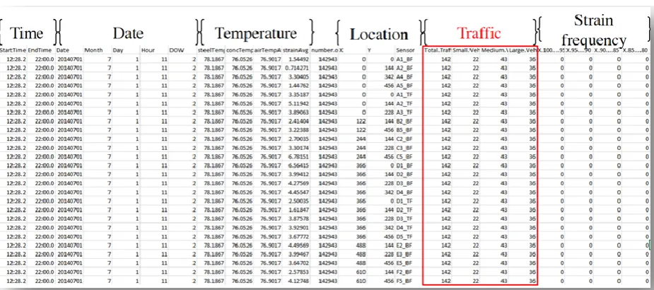
naturally produce a large number of strain peaks. The inclusion of traffic information can significantly improve the prediction of bridge strain responses. In this project, traffic flow data measured on Jordan Creek Parkway (by courtesy of Dr. Anuj Sharma) were merged into the bridge strain dataset. The traffic sensor data are measured every five minutes and have three categories: total counts of small, medium, and large vehicles within the time frame.

After merging bridge sensor and traffic sensor data, the resultant dataset would have the structure shown in Figure 6.

10

6 DATA CURING

In statistics, the theory of filling in missing values with statistically reliable values is called “imputation.” Data sets for bridge big data have many variables, a large size, and irregular patterns of missing data, and, importantly, there is little information about probabilistic

distributions of the variables. To overcome this challenge, this project adopted one of the most flexible and general imputation theories, i.e., fractional hot deck imputation (Kim and Fuller 2004). In particular, this project adopted the first author’s computational statistics package, which is open-source and downloadable from the global statistical platform R (see R package FHDI from http://CRAN.R-project.org/package=FHDI [Im et al. 2017]).

FHDI is an advanced statistical method to cure missing values. It has little need for statistical assumptions and prior knowledge about the data. FHDI creates donors (i.e., candidates for the missing value) by using imputation estimators (see Equations (1) and (2)). For one missing value, multiple donors are generated in view of joint probabilistic distributions of the raw data. In terms of donor selection methods, there are two imputation estimators: (1) the fully efficient fractional imputation (FEFI) estimator and (2) the FHDI estimator. FEFI uses all donors to cure missing values, while FHDI uses some selected donors. The kernel of FEFI is given by the following:

𝑌̂_{𝑖,𝐹𝐸𝐹𝐼} = ∑ ∑ 𝜔_𝑖{𝛿_𝑖𝑦_𝑖+ (1 − 𝛿_𝑝𝑖) ∑ 𝜔∗ 𝑖𝑗,𝐹𝐸𝐹𝐼 𝑗∈𝐴 𝑦𝑗} 𝑖∈𝐴𝑐

𝐶

𝑐=1 (1)

where 𝐴 is the index set of all samples; 𝐴𝑐 is the index set of a category; 𝜔𝑖 is the sampling

weight of the 𝑖-th recipient; 𝑦𝑖 is the 𝑖-th recipient; 𝛿𝑖 = 1 when 𝑦𝑖 is observed, otherwise 𝛿𝑖 =

0; and 𝜔∗_{𝑖𝑗,𝐹𝐸𝐹𝐼} is the fractional weight (see Im et al. 2015 for the theoretical details).

The kernel of FHDI is given by the following:

𝑌̂𝑖,𝐹𝐻𝐷𝐼 = ∑ ∑ 𝜔𝑖{𝛿𝑖𝑦𝑖+ (1 − 𝛿𝑝𝑖) ∑𝑀𝑗=1𝜔∗𝑖𝑗𝑦𝑖 ∗(𝑗)

}

𝑖∈𝐴𝑐

𝐶

𝑐=1 (2)

where 𝜔∗

𝑖𝑗 is the fractional weight for the FHDI estimator and 𝑦𝑖 ∗(𝑗)

is the 𝑖-th imputed value of

7 DATA PREDICTION

Because datasets for bridge big data have many variables, a large data size, and complex relationships among variables, the accurate prediction of bridge data is a formidable challenge. To overcome this challenge, this project adopted one of the most flexible and general statistical prediction methods, i.e., generalized additive model (Hastie and Tibshirani 1990).

7.1 Theoretical Summary of GAM

GAM is widely used as an advanced statistical model in statistical fields. Hitherto, it has rarely been used in the civil engineering field compared to traditional regression methods because it is relatively new and rarely understood. Therefore, it is instructive to expound upon the theoretical background of GAM prior to describing the in-depth applications.

GAM is a generalized linear model with strong flexibility and general applicability. It uses an unspecific smoothing function rather than predefined distributions or parametric relationships. Due to the unspecified smoothing function, the covariates (i.e., descriptive variables) do not need to have a set of parameters. GAM is formulated by predicting the target of the i-th sample

(denoted by 𝑌𝑖 ∈ ℝ) with n predictors (denoted by 𝒙𝑖𝑗 ∈ ℝ𝑛 where 1 ≤ 𝑗 ≤ 𝑛). The general

form of GAM can be represented as follows:

𝑌𝑖 = 𝑔(𝜇𝑖) = ∑ 𝑓𝑗 𝑗(𝑥𝑖𝑗) (3)

where 𝑔 is a smooth link function, the expectation of 𝑌𝑖 given 𝒙𝑖 is denoted by 𝜇𝑖 ≡ 𝔼(𝑌𝑖|𝒙𝑖),

𝑌_𝑖is a target response from an exponential family of distribution (e.g., normal, binomial, or gamma distribution), and 𝑓_𝑗 are smooth functions of covariates 𝑥_𝑗𝑖 (Wood 2006). Essentially, GAM has a nonparametric smooth function for each covariate. For simplicity, the following description includes a normal distribution single variable, but the generalization for multiple variables is straightforward (see Wood 2006). Let GAM be 𝔼(Y|𝑥) = 𝑓(𝑥), and the smoothing function 𝑓 can be represented as follows:

𝑓(𝑥) = ∑𝑘_𝑗=1𝑏_𝑗(𝑥)𝛽_𝑗

where 𝑏_𝑗 is the j-th basis function and 𝛽_𝑗 is an unknown parameter. The model can be fit by maximizing the corresponding likelihood. A penalty term is given as 𝜆 ∫[𝑓′′(𝑥)]2_{𝑑𝑥, where 𝜆 is}

the smoothing parameter. If λ is too large, it is an over-smoothed estimate, while it is an under-smoothed estimate if λ is too small. This error becomes greater at both extremes. The 𝜆 value is optimized by minimizing the generalized cross validation (GCV) score (Golub et al. 1979) and is automatically selected by the GAM library. Therefore, there is little need to manually adjust 𝜆.

12

Importantly, GAM’s internal setting always seeks to balance the fitting accuracy and smoothness, in which the generality and flexibility of GAM are rooted.

7.1.1 Excellent Performance of GAM Compared to ML

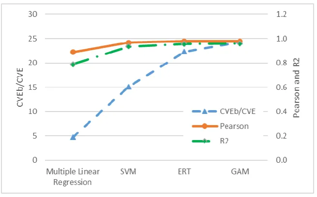
In addition to the flexibility of GAM, owing to the unspecified smoothing function, GAM also performs well in terms of prediction accuracy. In some of the authors’ previous work (Song et al. 2018), the prediction performance of GAM was compared to MLR and two popular machine learning algorithms (i.e., support vector machine [SVM] and extremely randomized trees [ERT]). Figure 7 shows the comparison result.

Adapted from Song et al. 2018

Figure 7. Comparison of prediction performance between GAM and other methods (i.e., multiple linear regression, SVM, and ERT)

On the vertical axes, a higher value indicates a higher prediction accuracy in terms of cross validation score ratio (CVEb/CVE), Pearson coefficient, and coefficient of determination (R2). GAM outperforms MLR and is slightly better than SVM and ERT.

Another advantage of GAM compared to ML is that the prediction result from GAM can be clearly explained based on statistical theories and methodologies while many ML methods are often unclear about the pathway between input and output. This issue is also known as “black-box” prediction of machine learning and “glass-“black-box” prediction of statistical learning. The advantage makes the adopted statistical prediction process more interpretable and enables researchers to build a better predictive model according to their knowledge about the data and pertinent engineering principles.

7.2 Direct Search Method for the Best Predictive Power

 Which variables are necessary for the best predictive power?

 Are all variables important for prediction?

14

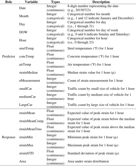
Table 2. Summary of predictor (explanatory) and response (target) variables used for the statistical prediction model

Role Variable Types Description

Predictor

Date Integer

(continuous)

8-digit number representing the date (e.g., 20150723)

Month Integer

(categorical)

Categorical number for month

(e.g., 1 and 12 indicate January and December)

Day Integer

(categorical)

Categorical number for day (i.e., 1 through 31)

DOW Integer

(categorical)

Categorical number for day of week

(e.g., 0 and 6 indicate Sunday and Saturday)

Hour Integer

(categorical)

Categorical number for hour (i.e., 0 through 23)

steelTemp Float

(continuous) Steel temperature (℉) for 1 hour

concTemp Float

(continuous) Concrete temperature (℉) for 1 hour

airTemp Float

(continuous) Air temperature (℉) for 1 hour

strainMedian Float

(continuous) Median strain value for 1 hour (µ)

nMeasurement Integer

(continuous) Count of strain measurement for 1 hour

smallCar Integer

(continuous) Traffic count by small size of vehicle for 1 hour

mediumCar Integer

(continuous)

Traffic count by medium size of vehicle for 1 hour

LargeCar Integer

(continuous) Traffic count by large size of vehicle for 1 hour

Response

strainMean Float

(continuous) Expected value of peak strain for 1 hour

strainMeanComp Float

(continuous)

Expected value of peak strain below the median strain for 1 hour

strainMeanTens Float

(continuous)

Expected value of peak strain above the median strain for 1 hour

strainMin Integer

(continuous) Minimum peak strain for 1 hour (µ)

strainMax Integer

(continuous) Maximum peak strain for 1 hour (µ)

strainSTD Float

(continuous) Standard deviation of peak strain (µ)

Area Integer

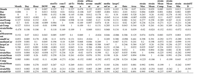
For the correlation-based selection method, the best predictors were chosen based on the correlation values. For instance, a correlation matrix that shows all variable-to-variable

16

Table 3. Correlations among all variables of bridge and traffic big data

Month Day Hour DOW

steelTe mp concT emp airTe mp strain Media n nMeas ureme nt smallC ar mediu mCar largeC

ar Date Area strain Max strain Mean strain Mean Comp strain Mean Tens strain Min strainST D Month 1 0.008 0 0.007 0.327 0.3 0.327 0.478 0.152 -0.053 0.039 0.103 0.396 0.07 0.034 0.029 0.085 0.031 0.013 0.035

Day 0.008 1 0 0.013 0.016 0.01 0.014 -0.106 0.07 0.005 -0.001 0.011 -0.03 0.012 0.004 0.005 0.001 0.004 0.002 0.005

Hour 0 0 1 0.001 0.152 0.186 0.145 0.106 0.012 0.178 0.1 0.34 -0.001 0.328 0.263 0.26 -0.102 0.278 -0.182 0.274

DOW 0.007 0.013 -0.001 1 -0.01 0.009 -0.01 0 0.043 -0.06 -0.045 0.114 0.008 -0.087 -0.058 -0.052 0.11 -0.027 0.092 -0.031

steelTemp 0.327 0.016 0.152 -0.01 1 0.984 0.998 0.118 0.085 0.13 0.196 0.131 0.001 0.341 0.277 0.258 -0.289 0.267 -0.24 0.285

concTemp 0.3 0.01 0.186 -0.009 0.984 1 0.98 0.169 0.097 0.074 0.18 0.111 0.02 0.287 0.236 0.216 -0.271 0.23 -0.211 0.246

airTemp 0.327 0.014 0.145 -0.01 0.998 0.98 1 0.109 0.1 0.131 0.205 0.119 0.043 0.344 0.28 0.261 -0.261 0.269 -0.224 0.286

strainMedia

n -0.478 0.106 0.106 0 0.118 0.169 0.109 1 0.069 0.011 0.068 0.134 0.16 0.039 -0.02 -0.024 -0.152 -0.011 -0.072 -0.011 nMeasurem

ent 0.152 0.07 0.012 0.043 0.085 0.097 0.1 0.069 1 -0.024 0.046 -0.086 0.306 0.125 0.074 0.076 0.083 0.075 0.003 0.072 smallCar 0.053 0.005 0.178 -0.06 0.13 0.074 0.131 0.011 -0.024 1 0.269 0.388 -0.096 0.461 0.398 0.391 -0.292 0.373 -0.289 0.393

mediumCar -0.039 0.001 0.1 0.045 0.196 0.18 0.205 0.068 0.046 0.269 1 0.467 0.151 0.241 0.2 0.198 -0.072 0.183 -0.099 0.191

largeCar 0.103 0.011 0.34 0.114 0.131 0.111 0.119 0.134 -0.086 0.388 0.467 1 0.246 0.384 0.267 0.26 -0.258 0.256 -0.257 0.262

Date 0.396 -0.03 0.001 0.008 -0.001 0.02 0.043 0.16 0.306 -0.096 0.151 -0.246 1 0.032 0.035 0.047 0.324 0.033 0.211 0.022

Area 0.07 0.012 0.328 0.087 0.341 0.287 0.344 -0.039 0.125 0.461 0.241 0.384 0.032 1 0.901 0.894 -0.266 0.881 -0.38 0.891

strainMax 0.034 0.004 0.263 -0.058 0.277 0.236 0.28 -0.02 0.074 0.398 0.2 0.267 0.035 0.901 1 0.994 -0.225 0.992 -0.282 0.995

strainMean 0.029 0.005 0.26 0.052 0.258 0.216 0.261 -0.024 0.076 0.391 0.198 0.26 0.047 0.894 0.994 1 -0.186 0.991 -0.254 0.992

strainMean

Comp 0.085 0.001 0.102 0.11 -0.289 -0.271 -0.261 -0.152 0.083 -0.292 -0.072 -0.258 0.324 0.266 -0.225 -0.186 1 -0.199 0.643 -0.237 strainMean

Tens 0.031 0.004 0.278 -0.027 0.267 0.23 0.269 -0.011 0.075 0.373 0.183 0.256 0.033 0.881 0.992 0.991 -0.199 1 -0.262 0.997 strainMin 0.013 0.002 -0.182 0.092 -0.24 -0.211 -0.224 -0.072 0.003 -0.289 -0.099 -0.257 0.211 -0.38 -0.282 -0.254 0.643 -0.262 1 -0.293

For the authors’ direct search method, all possible combinations were examined without any prejudice regarding predictors and responses. For example, when a seven-variable prediction model was constructed, the authors considered 1,716 combinations in total (i.e., [13!/7!(13-7)!]), and all cases were separately constructed and compared. The computation cost, therefore, is highly expensive. Therefore, a HPC algorithm was developed using Rmpi (an HPC library for R code) to distribute computations over multiple CPUs.

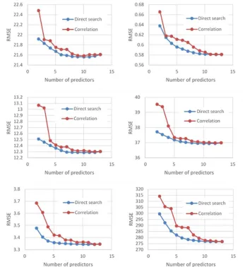
The comparison of the prediction performances between the correlation-based selection and the direct search method is shown in Figure 8.

Figure 8. Comparison of prediction errors generated by direct search method and correlation-based selection

18

Table 4. Best combinations of predictors selected by the direct search method

Prediction target

# of predic

tors Best Combination of Predictors (p-value)

strainMeanTop 10

Month(4.91e-9) airTemp(4.80e-7) smallCar(9.15e-11) Date(2.26e-11) Hour(< 2e-16) strainMedian(4.22e-5) mediumCar(0.106) concTemp(1.09e-6) nMeasurement(< 2e-16) largeCar(3.24e-15) strainMeanBott

om 12

Month(< 2e-16) DOW(< 2e-16) airTemp(< 2e-16) smallCar(2.63e-9) Day(0.02626) steelTemp(< 2e-16) strainMedian(< 2e-16) mediumCar(0.00224) Hour(< 2e-16) concTemp(3.06e-12) nMeasurement(< 2e-16) Date(< 2e-16)

strainSTD 10

Month(4.32e-9) airTemp(2.89e-7) smallCar(3.41e-13) Date(2.39e-10) Hour(< 2e-16) strainMedian(2.92e-5) mediumCar(0.191) concTemp(3.05e-7) nMeasurement(< 2e-16) largeCar(9.10e-12)

strainMax 11

Month(5.52e-11) concTemp(1.39e-6) nMeasurement(< 2e-16) largeCar(2.34e-10) Hour(< 2e-16) airTemp(2.49e-6) smallCar(8.14e-10) Date(3.78e-10) DOW(9.81e-15) strainMedian(2.46e-5) mediumCar(0.27)

strainMin 12

Month(5.42e-6) DOW(< 2e-16) airTemp(8.12e-7) mediumCar(0.025373) Day(0.364342) steelTemp(1.22e-12) nMeasurement(< 2e-16) largeCar(0.007920) Hour(< 2e-16) concTemp(0.000649) smallCar(0.072332) Date(< 2e-16)

Area 12

Month(< 2e-16) DOW(< 2e-16) strainMedian(3.73e-10) mediumCar(0.00458) Day(5.05e-4) concTemp(< 2e-16) nMeasurement(< 2e-16) largeCar(< 2e-16) Hour(< 2e-16) airTemp(2.41e-15) smallCar(1.06e-8) Date(6.98e-13)

Small car traffic 15

Month(< 2e-16) DOW(< 2e-16) airTemp(8.95e-7) Area(5.41e-13) strainMeanTop(2.50e-15) Day(4.46e-13) steelTemp(9.69e-7) strainMedian(4.19e-4) strainMax(1.27e-4) strainMin(1.96e-7 ) Hour(< 2e-16) concTemp(3.75e-5) Date(< 2e-16) strainMeanBottom.(1.04e -4) strainSTD(4.71e-16) Medium car

traffic 13

Month(< 2e-16) DOW(< 2e-16) airTemp(< 2e-16) Date(< 2e-16) strainSTD(7.70e-8) Day(< 2e-16) steelTemp(3.17e-12) strainMedian(< 2e-16) Area(9.07e-7) Hour(< 2e-16) concTemp(2.39e-12) nMeasurement(0.2495) strainMax(0.0122)

Large car traffic 14

20

 Bridge big data can be predicted by a statistical prediction model with a number of variables.

 The direct search algorithm can identify the best combination of predictors that can lead to the best predictive power.

 Not all variables are necessarily needed for predicting future bridge sensor data.

7.3 Prediction of Traffic Flow Data

In the preceding section, the direct search method was investigated to find the best predictor combination for six target responses. The same approach is applied to investigate the application of bridge sensor data to the prediction of traffic data. Here, the previous six target responses related to strain are considered as predictors, and three traffic variables (i.e., traffic of small, medium, and large car sizes) are treated as target responses. Best predictors for three targets (i.e., (a) small vehicles, (b) medium vehicles, and (c) large vehicles) are shown in Figure 9.

Figure 9. Variation of prediction errors with different combination of predictors during traffic flow data prediction

The traditional assumption is that the more predictors that are used, the higher the prediction accuracy that can be expected. But the highest accuracy is not necessarily guaranteed when all predictors are used. In particular, the authors found that the numbers of the best predictor

combinations for GAM turned out to be 15, 13, and 14 out of a total of 16 variables for the small, medium, and large car sizes, respectively. Those selected predictors are listed in Table 4.

Figure 10. Quantile-quantile (Q-Q) plots of the original traffic data and the predicted traffic data: (a) small vehicles (R2 _{= 0.77), (b) medium vehicles (R}2 _{= 0.44), (c) large vehicles}

(R2 _{= 0.70)}

Straight overlapped lines in the Q-Q plots in Figure 10 indicate better prediction. Using the bridge big data, the developed program appears to have reasonable prediction performance for small and large vehicles, with R2, the coefficient of determination, greater than 0.7. Relatively, prediction of the traffic flow of medium vehicles appears to need improvement, with R2 around 0.44. The prediction error may be attributed to the short time period of the bridge big data, i.e., less than three years.

Although the prediction accuracy calls for further improvement, this project provides meaningful development and foundational conclusions, including the following:

 Bridge big data can be used to predict traffic flow in long-term time periods.

 Direct search algorithms can identify the best combination of predictors that lead to the best predictive power.

22

8 VARIOUS IMPACTS ON DATA PREDICTION

8.1 Impact of Data Curing on Data Prediction

Data measured from sensors typically have missing values for various reasons (e.g.,

measurement error or malfunction of sensors), which can lead to a significant lack of data for data analysis. The FHDI method was adopted in this study to address this issue. The six

prediction targets used in the previous chapter were used to compare the prediction performance of GAM between the datasets with and without data curing using FHDI. Figure 11 shows the results of the comparison of prediction performance. The RMSE values from the prediction results using the dataset without imputation are normalized by the RMSE values from the prediction results using the imputed dataset. The prediction errors are slightly lower when using the imputed dataset.

Figure 11. Comparison of prediction performance of GAM when using bridge big data after data curing by imputation (blue-colored bars) and before data curing, i.e., with

missing data (orange-colored bars)

8.2 Impact of Inclusion of Traffic Data on the Prediction of Bridge Data

Figure 12. Comparison of prediction performance of GAM when using bridge big data after merging with traffic data (blue-colored bars) and without traffic data (orange-colored

24

9 INVESTIGATION INTO NEW DATA SOURCE – SURFACE SENSORS

The developed data processing tool can handle information from existing bridge strain sensors. The sensor data are defined at specific locations, and thus researchers are aware of point-wise strain information on the bridge. With the advent of surface strain sensors, such point-wise information can be extended to continuous strain information over the entire bridge plate.

To prepare for such new sources of dense and continuous information, this project conducted foundational investigations into advanced surface sensors. Understanding such surface sensors will facilitate the use of dense data to improve the predictive power of the models developed in this project for the long-term spatiotemporal behavior of bridges and for traffic flow.

This section summarizes the research team’s approach to investigating new surface sensors and presents meaningful findings obtained from initial experiments.

9.1 Background on Surface Sensors

Carbon fiber-reinforced polymer (CFRP) materials have been widely used for strengthening (Chen and Davalos 2010), rehabilitating, and retrofitting (Ray et al. 2010) structures. Over the last few decades, structural health monitoring using CFRPs has been a subject of increasing interest. For example, CFRPs can be used as a self-sensing material by leveraging the carbon fibers’ piezoresistive effect (Abry 1999, Irving 1998, Kaddour 1994, and Todoroki 2004). Recent research has used CFRP to produce structural capacitors, where strain can be measured as a change in capacitance. Chung and Wang (1999) proposed a capacitor fabricated from semi-conductive carbon fibers and an insulation paper for the dielectric. Luo and Chung (2001) proposed using CFRP layers as electrodes, also separated by insulation paper, which could provide a capacitance up to 1,200 nF/m2. Inspired by the promising use of CFRPs as structural capacitors, researchers have focused on the improvement of the capacitance by introducing different separators (O’Brien et al. 2011) and modifying the treatment of surface electrodes (Qian et al. 2013). The aforementioned studies mainly focused on enhancing the capacitance of the materials. Few studies have focused on electromechanical applications. Carlson and Asp (2014) studied the effect of damage on the electrical properties of a structural capacitor that used polyethylene terephthalate (PET) as the dielectric. They reported that the capacitance remained unchanged after significant interlaminar matrix cracking in the CFRP electrodes. Shen and Zhou (2017) noted that interlaminar damage can instead lead to a reduction in capacitance and

modeled the capacitance as a function of interfacial cracking. This behavior is unlike that of other types of structural capacitors for SHM found in the literature (Laflamme et al. 2013), where the capacitance increases following strain.

MBrace® CF 130 fabric and MBrace® Saturant (BASF Chemical Corporation) were used to fabricate electrode plates with a unidirectional carbon fiber pattern, with an ultimate tensile strength of 3,800 MPa. The dielectric was fabricated using Mbrace® Saturant filled with polydimethylsiloxane (PDMS)-coated titania (TPL, Inc.), a high-permittivity filler. The mechanical properties of the CFRP components are listed in Table 5.

Table 5. Mechanical properties of CFRP components provided from the supplier

Component

Ultimate Tensile Strength (Mpa)

Young’s Modulus (GPa)

Ultimate Rupture Strain

Fiber 4,950 - -

Saturant 55.2 3.034 3.5%

Cured CFRP 3,800 227 1.67%

9.2 Surface Sensor Fabrication

The capacitive CFRP sensor is composed of two conductive electrodes separated by a dielectric. It is fabricated using the following two steps:

1. Fabricate CFRP electrodes plates. The epoxy is first mixed using a mixing machine

homogenizer (Figure 13(a)). The uncured saturant is applied onto the fabric and cured using a vacuum bagging process (Figure 13(b)) to obtain good mechanical and electrical properties. To form a better connection to the data acquisition (DAQ) component for capacitance

measurement, two copper tapes with conductive adhesive are attached onto the fabric surface before applying the epoxy. The surface of the copper tape is polished with sandpaper after curing. After the electrode plate is cured for 24 hours, plates are cut from the middle section where the thickness is uniform.

2. Separate the CFRP plates with the dielectric. A separator is made with the same epoxy used in Step 1 but filled with 5% titania by weight (Figure 13(c)). The epoxy is applied onto the plates (Figure 13(d)) and cured using vacuum bagging for 24 hours.

26

Figure 13. Sensor fabrication process

9.3 Experiment Setup and Instrumentation of Surface Sensor

The experimental setup is shown in Figure 14.

The CFRP specimens were 177.8 mm (7 in) long by 25.4 mm (2 in) wide, with thicknesses varying between specimens (reported in Table 6). Fiberglass strips were adhered to the ends of the specimens to insulate the electrode from the hydraulic grip and prevent crushing. A load was applied using a servo-hydraulic material testing system (MTS) machine under displacement control at a loading rate of 2 mm/min. Loads and displacements were acquired from the MTS at a sampling frequency of 10 Hz. CFRP capacitance measurement was performed using an LCR meter (HP 4284A) under 1 kHz. The thicknesses and electrical properties of the three specimens were measured before initiating the tests.

The test results are listed in Table 6, in which the relative permittivity er was back-calculated

from the initial geometries.

Table 6. Specimen configuration

Specimen Thickness (mm) Initial capacitance (pF) Relative permittivity (er)

# 1 2.64 251.4 16.60

# 2 2.57 266.1 17.10

# 3 2.36 340.8 20.11

The difference in the relative permittivity values is attributed to the manual fabrication process. Specimen #3 was equipped with a resistive strain gauge (RSG) to obtain an experimental value for the gauge factor. The RSG consisted of a foil gage sampled at 10 Hz using a Vishay Model 5100 B Scanner DAQ.

9.4 Results and Discussion of Surface Sensor Tests

28

Figure 15. Surface sensor test results for force and stress versus strain curves

The experimental Young’s modulus values of the CFRP-based capacitors are summarized in Table 7. The Young’s modulus values of three specimens average 47.9 GPa.

Table 7. Specimen test results

Specimen Young’s Modulus (GPa) Fracture strain (%)

# 1 45.0 4.4

# 2 45.3 1.5

# 3 53.3

Figure 16. Surface sensor test results showing the failure modes of the specimens, from left to right, Specimen #1, Specimen #2, Specimen #3

30

Results show an increase in capacitance with increasing strain, with the similar slopes among each specimen in the linear range. Specimen #3 exhibits a nonlinear relationship between capacitance and strain beyond approximately 1% strain, which can be attributed to the

delamination of the CFRP. This behavior was confirmed by an audible cracking of the specimen during testing, indicating possible delamination of the CFRP.

The experimental gauge factor was calculated using the strain values measured directly from the RSG, because the strain back-calculated from the MTS displacement values may not reflect the behavior of the specimens accurately enough. Figure 18 plots the relative capacitance versus strain from the RSG for Specimen #3 (the only specimen equipped with an RSG) before crushing of the tabs occurred.

Figure 18. Relative capacitance versus RSG strain, Specimen #3

The linear fit shows a gauge factor of 1.066. Typical Poisson’s ratio values vxy and vxz for the

utilized CFRP and saturant are 0.27 and 0.4, respectively, yielding an analytical gauge factor of approximately 1.13. Note that this value has a certain variability due to the unreported value of vxy from the manufacturer and the addition of titania in the saturant. It follows that the

experimental gauge factor is in agreement with theory.

32

10 DOWNLOADABLE PROGRAMS AND DATA

10.1 Data Processing Programs

Download Location: https://iastate.box.com/s/4sr1eur3wfcirzk9t5q0b3yabtptb78u

 All programs and computational tools developed in this project are publicly available. Data transferring, data squashing, data merging, and relevant parallel computing code and programs are downloadable from the web folder listed above. A brief manual explaining the use of the programs is also available in the web folder.

10.2 Final Datasets

Download Location: https://iastate.box.com/s/wh12iz8d7skjho7obcefjg7hpjz8apbz

 Database/Traffic/traffic_transformed_data

This folder contains traffic data for each year starting from 2014 through 2016. The traffic data have been transformed for synchronization with bridge big data.

 Database/Traffic/traffic_original_data

This folder contains the raw traffic data in its original format. These raw traffic data are shared by Dr. Anuj Sharma’s research group by courtesy.

 Database/1-hour_dataset

This folder contains the final hybrid data from the bridge sensors and traffic data

synchronized for a one-year time frame. Each “.csv” file corresponds to one year of data for a sensor. Note that this dataset may have missing values due to incomplete raw data from the bridge sensor database.

 Database/1-hour_dataset_imputation

This folder contains the final hybrid data from the bridge sensors and traffic data

11 CONCLUSIONS

With the persistent advances in bridge sensors and traffic sensors, researchers have novel access to big data in various forms, including for structural behavior and transportation information. Big data-oriented problems pose formidable challenges for big data-driven decision-making and efficient long-term strategic planning. To overcome these obstacles, this project developed a foundational computational framework to leverage bridge big data and traffic data in predicting the long-term behavior of bridges and traffic flows. This project created a suite of computational methods and tools that can perform multiple functions for data-driven bridge data prediction.

The developed programs include the following:

 A data-squashing tool that can transform and reduce original bridge sensor data to manageable sizes

 A data-curing tool that can fill in many missing values in original datasets regardless of data type and size

 A data-merging tool that can synchronize bridge big data and traffic flow data

 A data-prediction tool that can predict both bridge-related data as well as traffic flow

In tandem, this project conducted an experimental investigation into the new data source of dense surface sensors. The surface sensor developed in this study can provide continuous and highly refined data for use in the developed computational foundation. In terms of the generality of the developed framework, the inclusion of more data and other types of data, such as data from surface sensors, will be straightforward in future extensions of the framework.

By utilizing all of the developed programs, this project yielded several practically meaningful findings:

 Not all variables are necessarily helpful for improving predictive power.

 For the best predictive power, a direct search of the optimal combination of variables is necessary.

 A simple correlation-based selection of significant variables may lead to relatively low predictive power.

 Curing missing data in the original datasets helps improve predictive power.

 Merging traffic data into bridge big data improves predictive power.

 Bridge big data can be predicted by using traffic data, and, in turn, traffic data can be predicted by using bridge big data.

All the developed programs are shared with practitioners and researchers via web folders.

34

REFERENCES

Abry, J. C., S. Bochard, A. Chateauminois, M. Salvia, and G. Giraud. 1999. In situ detection of damage in CFRP laminates by electrical resistance measurements. Composites Science and Technology, Vol. 59, No. 6, pp. 925–935.

Carlson, T. and L. Asp. 2014. An experimental study into the effect of damage on the

capacitance of structural composite capacitors. Journal of Multifunctional Composites, Vol. 2, No. 2, pp. 71-77.

Chen, A. and J. Davalos. 2010. Strength evaluations of sinusoidal core for FRP sandwich bridge deck panels. Composite Structures, Vol. 92, No. 7, pp. 1561–1573.

Chung, D. D. L. and S. Wang. 1999. Carbon fiber polymer-matrix structural composite as a semiconductor and concept of optoelectronic and electronic devices made from it. Smart Materials and Structures, Vol. 8, No. 1, pp. 161–166.

Golub, G. H., M. Heath, and G. Wahba. 1979. Generalized cross-validation as a method for choosing a good ridge parameter. Technometrics, Vol. 21, No. 2, pp. 215–223.

Hastie, T. J. and R. J. Tibshirani. 1990. Generalized additive models. Monographs on Statistics and Applied Probability 43. Chapman and Hall, CRC Press, Boca Raton, FL.

Im, J., J.-K. Kim, and W. A. Fuller. 2015. Two-phase sampling approach to fractional hot deck imputation. In Proceedings of the Survey Research Methods Section, American Statistical Association, pp. 1030–1043.

Im, J., Cho, I., and J. Kim. 2017. FHDI: Fractional Hot Deck and Fully Efficient Fractional Imputation. R package version 1.0. http://CRAN.R-project.org/package=FHDI. Irving, P. E. and C. Thiagarajan. 1998. Fatigue damage characterization in carbon fibre composite materials using an electrical potential technique. Smart Materials and Structures, Vol. 7, No. 4, pp. 456–466.

Jang, S., H. Jo, S. Cho, K. Mechitov, J. A. Rice, S.-H. Sim, H.-J. Jung, C.-B. Yun, B. F. Spencer, Jr., and G. Agha. 2010. Structural health monitoring of a cable-stayed bridge using smart sensor technology: deployment and evaluation. Smart Structures and Systems, Vol. 6, No. 5-6, pp. 439–459.

Kaddour, A., F. Al-Salehi, S. Al-Hassani, and M. Hinton. 1994. Electrical resistance measurement technique for detecting failure in CFRP materials at high strain rates. Composites Science and Technology, Vol. 51, No. 3, pp. 377–385.

Kim, J. K. and W. Fuller. 2004. Fractional hot deck imputation. Biometrika, Vol. 91, No. 3, pp. 559-578.

Ko, J. and Y. Ni. 2005. Technology developments in structural health monitoring of large-scale bridges. Engineering Structures, Vol. 27, No. 12, pp. 1715–1725.

Laflamme, S., H. Saleem, B. Vasan, R. Geiger, D. Chen, M. Kessler, and K. Rajan. 2013. Soft elastomeric capacitor network for strain sensing over large surfaces. IEEE/ASME Transactions on Mechatronics, Vol. 18, No. 6, pp. 1647–1654.

Le, T. and H. D. Jeong. 2017. NLP-Based Approach to Semantic Classification of

Heterogeneous Transportation Asset Data Terminology. Journal of Computing in Civil Engineering, Vol. 31, No. 6, pp. 04017057-1–04017057-13.

36

Li, Z., T. H. Chan, and R. Zheng. 2003. Statistical analysis of online strain response and its application in fatigue assessment of a long-span steel bridge. Engineering Structures, Vol. 25, No. 14, pp. 1731–1741.

Luo, X. and D. D. L. Chung. 2001. Carbon fiber/polymer matrix composites as capacitors. Composites Science Technology, Vol. 61, No. 6, pp. 885–888.

Lv, Y., Y. Duan, W. Kang, Z. Li, and F.-Y. Wang. 2015. Traffic flow prediction with big data: a deep learning approach. IEEE Transactions on Intelligent Transportation Systems, Vol. 16, No. 2, pp. 865–873.

Ntotsios, E., C. Papadimitriou, P. Panetsos, G. Karaiskos, K. Perros, and P. C. Perdikaris. 2009. Bridge health monitoring system based on vibration measurements. Bulletin of

Earthquake Engineering, Vol. 7, No. 2, pp. 469–483.

O’Brien, D. J., D. M. Baechle, and E. D. Wetzel. 2011. Design and performance of

multifunctional structural composite capacitors. Journal of Composite Materials, Vol. 45, No. 26, pp. 2797–2809.

Perera, L. P. and B. Mo. 2016. Data compression of ship performance and navigation

information under deep learning. Paper presented at the 35th International Conference on Ocean, Offshore and Arctic Engineering (OMAE 2016), June 19–23, Busan, Korea. Qian, H., A. Kucernak, E. Greenhalgh, A. Bismarck, and M. Shaffer. 2013. Multifunctional

Structural Supercapacitor Composites Based on Carbon Aerogel Modified High

Performance Carbon Fiber Fabric. ACS Applied Materials and Interfaces, Vol. 5, No. 13, pp. 6113–6122.

Ray, I., G. C. Parish, J. F. Davalos, and A. Chen. 2010. Effect of concrete substrate repair methods for beams aged by accelerated corrosion and strengthened with CFRP. Journal

of Aerospace Engineering, Vol. 24, No. 2, pp. 227–239.

Shen, Z. and H. Zhou. 2017. Mechanical and electrical behavior of carbon fiber structural capacitors: Effects of delamination and interlaminar damage. Composite Structures, Vol. 166, pp. 38–48.

Song, I., I.-H. Cho, and R. Wong. 2018. An Advanced Statistical Approach to Data-Driven Earthquake Engineering. Journal of Earthquake Engineering. (under review).

Todoroki, A. and J. Yoshida. 2004. Electrical resistance change of unidirectional CFRP due to applied load. JSME International Journal Series A, Vol. 47, No. 3, pp. 357–364. Wood, S. 2006. Generalized additive models: an introduction with R. First Edition. Chapman

Visit www.InTrans.iastate.edu for color pdfs of this and other research reports.

THE INSTITUTE FOR TRANSPORTATION IS THE FOCAL POINT FOR TRANSPORTATION AT IOWA STATE UNIVERSITY.

InTrans centers and programs perform transportation research and provide technology transfer services for government agencies and private companies;

InTrans manages its own education program for transportation students and provides K-12 resources; and