A Family of Variable Step-Size Normalized Subband Adaptive Filter Algorithms Using Statistics of System Impulse Response

A Family of Variable Step-Size Normalized Sub-Band

Adaptive Filter Algorithms using Statistics of System Impulse

Response

M. Shams Esfand Abadi and M. S. Shafiee

Abstract: This paper presents a new Variable Step-Size Normalized Subband Adaptive Filter (VSS-NSAF) algorithm. The proposed algorithm uses the prior knowledge of the system impulse response statistics and the optimal step-size vector is obtained by minimizing the Mean-Square Deviation (MSD). In comparison with NSAF, the VSS-NSAF algorithm has faster convergence speed and lower MSD. To reduce the computational complexity of VSS-NSAF, the VSS Selective Partial Update NSAF (VSS-SPU-NSAF) is proposed where the filter coefficients are partially updated in each subband at every iteration. We demonstrated the good performance of the proposed algorithms in convergence speed and steady-state MSD for a system identification set-up.

Keywords: Adaptive filter, Normalized Subband Adaptive Filter (NSAF), Selective Partial Update (SPU), Variable Step-Size (VSS).

1 Introduction0F1

Adaptive filtering has been, and still is, an area of active research that plays an active role in an ever increasing number of applications, such as noise cancellation, channel estimation, channel equalization and acoustic echo cancellation [1-5]. The Least Mean Square (LMS) and its normalized version (NLMS) are the workhorses of adaptive filtering. In the presence of colored input signals, the LMS and NLMS algorithms have extremely slow convergence rates. Adaptive filtering in subbands has been proposed to improve the convergence behavior of the LMS algorithm [6]. The normalized subband adaptive filter (NSAF) was proposed in [7]. In [8], the selective partial update NSAF (SPU-NSAF) was proposed to reduce the computational complexity. In this algorithm, the filter coefficients are partially updated in each subband at every iteration. This feature leads to the reduction in computational complexity. Other selective partial update adaptive filter algorithms can be found in [9, 10].

In above mentioned algorithms, the selected fixed step-size can change the convergence rate and the steady-state Mean Square Error (MSE). It is well known that the steady-state MSE decreases when the step-size

Iranian Journal of Electrical & Electronic Engineering, 2013. Paper first received 28 Jan. 2013 and in revised form 23 Feb. 2013. * The Authors are with the Faculty of Electrical and Computer Engineering, Shahid Rajaee Teacher Training University, P.O.Box: 16785-163, Tehran, Iran, Tel/Fax: +98-21-22970003.

Emails: [email protected], [email protected].

decreases, while the convergence speed increases when the size increases. By optimally selecting the step-size during the adaptation, we can obtain both fast convergence rate and low steady-state MSE. In [11], a new variable-step-size control was proposed for the Normalized Least-Mean-Square (NLMS) algorithm. A step-size vector with different values for each filter coefficients was used in [11]. In this approach, based on the prior knowledge of the system impulse response statistics, the optimal step-size vector is obtained by minimizing MSD. In [12], the approach of [11] was extended to NSAF. But the computational complexity of the presented algorithm was high.

In this paper, we extend the approach in [11] to SPU-NSAF algorithm and VSS version of this algorithm is proposed. In the proposed algorithm, the step-size changes during the adaptation and the coefficient are partially updated at every iteration. We demonstrate the good performance of the presented algorithms through several simulation results in a system identification scenario. Also, the computational complexity of all algorithms is compared and analyzed. Furthermore, the performance of the proposed VSS-NSAF is compared with other VSS-VSS-NSAF algorithms in [8, 13].

We have organized our paper as follows. In Section 2, we briefly review NSAF, and SPU-NSAF algorithms. In Section 3, the proposed VSS adaptive algorithms are established. Section 4 presents the computational complexity of the algorithms. Finally, before concluding

the paper, we demonstrate the usefulness of these algorithms by presenting several experimental results. Throughout the paper, the following notations are adopted:

.

Norm of a scalar. 2

.

Squared Euclidean norm of a vector. 2

∑

t

∑-Weighted Euclidean norm of a column

vector

t

defined as

t

T

∑

t

_.

{}

.

E

Expectation operator.

( )

T

.

Transpose of a vector or a matrix.

(.)

diag

Has the same meaning as the MATLAB operator with the same name: If its argument is a vector, a diagonal matrix with the diagonal elements given by the vector argument results. If the argument is a matrix, its diagonal is extracted into a resulting vector.

2 Background on Nsaf and Spu-Nsaf Algorithms Adaptive filtering in subbands has been proposed to improve the convergence behavior of the LMS algorithm [6, 14]. In subband adaptive filtering, the input signal and desired response are band-partitioned into almost mutually exclusive subband signals. This feature of the SAF permits the manipulation of each subband signal, in such a way that their properties can be exploited [2], allowing each subband to converge almost separately for various modes [6], and thus improving the overall convergence behavior. In this section we briefly review NSAF and SPU-NSAF algorithms.

2.1 NSAF Algorithm

Fig. 1 shows the structure of NSAF [7]. In this figure, f0, f1, …, fN-1, are analysis filter unit impulse responses of an N channel orthogonal perfect reconstruction critically sampled filter bank system.

) (n i

x and d_i(n)are nondecimated subband signals. It is important to note that n refers to the index of the original sequences and k denotes the index of the decimated sequences. Similar to the NLMS algorithm, NSAF can be established by the solution of the following optimization problem

2 ) ( ) 1 (

min w k+ − w k

(1)

subject to the set of N constraints imposed on the decimated filter output

1 ,..., 0 )

1 ( ) ( ) (

,D k = Ti k k+ for i= N−

i

d x w (2)

where:

[

( ), ( 1),..., ( 1)

]

)

(k = x_i kN x_i kN− x_i kN−M+

i

x ₍₃₎

By solving this optimization problem based on the method of Lagrange multipliers, the filter update equation for NSAF can be stated as [7].

∑− = + =

+ 1

0 ( )2 ) ( , ) ( )

( ) 1

( N

i _i k

k D i e k i k

k _x

x

w

w

μ ₍₄₎

where e_i,D(k)=d_i,D(k)− wT(k)x_i(k) is the decimated subband error signal, and µ is the step size which is chosen in the range 0<μ<2 [7]. We also assumed a linear data model for the desired signal as:

) ( , ) ( ) (

,D k Ti k o viD k i

d = x w + (5)

where w0 is the true unknown filter vector, and vi,D(k)

is partitioned and decimated additive noise with zero mean and variance, 2

,D i v

σ . We also assume that v(n) is identically and independently distributed (i.i.d.) and statistically independent of the input data x(n).

2.2 SPU-NSAF Algorithm

To reduce the computational complexity of NSAF, SPU-NSAF algorithm was proposed in [8]. Partition

) (k i

x

1

0≤i≤N−

for and w (k) into B blocks each of

length L which are defined as

[

]

T

k T

B i k T i k T i k

i( ) x _,1( ),x _,2( ),...,x _, ( )

x

= (6)

[

]

T

k T B k T k T

k) ₁( ), ₂( ),..., ( )

( w w w

w

= ₍₇₎

Suppose we want to update S blocks out of B blocks in each subband at every adaptation. Let

{

j j j_s

}

F= ₁, ₂,..., denote the indexes of the S blocks out of B blocks. In this case, the optimization problem is defined as

Fig. 1 Structure of NSAF algorithm

2 ) ( ) 1 ( ) 1 (

min _F k _F k k

F

w

w

w + −

+ (8)

Subject to Eq. (2). By using the Lagrange multipliers approach, the filter vector update equation is given by

∑− = + =

+ 1

0 _{( )}2

, ) ( , ) ( , ) ( ) 1 ( N i _k F i k D i e k F i k F k F x x w w μ ₍₉₎

where _iF k =

⎡

⎢⎣

T_{i j} (k), _iT_,j2(k),..., T_i,js(k)

⎤

⎥⎦

T 1 , ) ( , x x x x . To reduce the computational complexity associated with the selection of the blocks to update, two alternative simplified criteria were proposed: 1) In the first approach, we compute the following Values

∑− = ≤ ≤ 1 0 1 2 ) ( , N

i ib k for b B

x

(10)

The indexes of the set F correspond to the indexes of the S largest values of Eq. (10). 2) In the second approach, we identify a set of indexes, correspond to the S smallest values of Eq. (11) [8].

⎪⎭

⎪

⎬

⎫

⎪⎩

⎪

⎨

⎧

∑− = ≤ ≤ = 1

0 _, ( ) 2 2 ) ( , 1min arg N

i _ib k

k D i e B b

j _x (11)

3 Derivation of Vss-Nsaf and Vss-Spu-Nsaf Algorithms

In this section, we establish the family of VSS-NSAF algorithms based on [11]. This method minimizes MSD and obtains the step-size vector based on the system impulse response statistics.

3.1 VSS-NSAF Algorithm

The update equation for VSS-NSAF is introduced as: ∑− = + = + 1

0 ( )2 ) ( , ) ( ) ( ) ( ) 1 ( N

i _i k

k D i e k i k k k _x x U w w (12)

where U(k)=diag

[

μ₀(k),...,μ_M−1(k)

]

is the variable step-size matrix. During the adaptation, this matrix changes to obtain faster convergence speed and lower steady-state MSD. Therefore, the objective of this paper is to design the step-size matrix U(k) to improve the performance of the NSAF algorithm. By defining the weight error vector as:

) ( )

(

~w _{k =} w _o− w _{k (13)}

and using the definition of e_i,D(k), the decimated error signal can be rewritten as:

) ( , ) ( ) ( ~ ) (

,D k T k i k vi D k i

e = w x + (14)

Now by substituting Eqs. (13, 14) into Eq. (12), we obtain: ∑− = − = + 1

0 ( )2 ) ( , ) ( ) ( ) ( ~ ) ( ) 1 ( ~ N

i _i k

k D i v k i k k k k _x x U w A w (15) where: ∑− = − = 1

0 ( ) 2

) ( ) ( ) ( ) ( N

i _i k

k T i k i k M k _x x x U I A (16)

and IM is the M×M identity matrix. To quantitatively evaluate the mis-adjustment of the filter coefficients, the MSD is taken as a figure of merit, which is defined as:

[

~_{( )} 2

]

)

(k =E w k

Λ (17)

Note that at each iteration, the MSD depends on

) (k j

μ . Combining Eqs. (15) and (17), we obtain:

[

~ ( ) ( ) ( )~( )

]

) 1

( + = +γ

Λ k E w T k A T k A k w k (18)

where:

[ ]

_∑− = = 1 0 2 2 , 2 ) ( 2 _N i i x D i v M k Tr σ σ γ U (19)

Similar to [13], we assume again that x_i(kN)and

) ( ,D k i

v are zero-mean i.i.d. stationary with variance

2

i X

σ and 2 ,D i v

σ , respectively; ~w (k), x_i(kN), and

) ( ,D k i

v are mutually independent and

1 2

) ( )

( ≈ for M >>

i x M k i k T i σ x x

. Therefore, we Obtain:

[

]

[ ]

2 ( )

2 ) ( 2 1 ) ( ) ( k M N M I M k NTr k k T E U U A A − + =

⎭

⎬

⎫

⎩

⎨

⎧

(20)

Combining Eqs. (18) and (20), we get:

[ ]

[

]

[

]

+γ

− + = + Λ

⎭

⎬

⎫

⎩

⎨

⎧

) ( ~ ) ( ) ( ~ 2 2 ) ( ~ 2 ) ( 2 1 ) 1 ( k k k T E M N k E M k NTr k w U w w U (21)

The optimal step size is obtained by minimizing the MSD at each iteration. Taking the first-order partial derivative of Λ(k+1) with respect to

(

0, , 1

)

)

(k j= M−

j K

μ , we will have

[

]

[

]

∑− = + − = ∂ + Λ ∂ 1 0 2 , 2 ) ( 2 2 ) ( ~ 2 2 ) ( 2 2 ) ( ~ ) ( ) 1 ( N i i x D i v k j M k j w E M N M k j N k E k j k σ σ μ μ μ w (22)

Setting Eq. (22) to zero, we obtain:

[

]

[

]

∑− = + = 1 0 2 , 2 2 ) ( ~ ) ( ~ ) ( N i i x D i v k NE k j w NME k j σ σ μ w (23)

To update E

[ ]

w~2_j(k) , we use the following equation obtained by taking the mean square of the k-th entry in Eq. (15).

[

]

[

]

[ ]

[

]

∑− = + + − = + 1 0 2 2 , 2 ) ( 2 2 ) ( ~ 2 ) ( 2 ) ( 2 ~ ) ( 2 1 ) 1 ( 2 ~ N i i x D i v M k j k E M k j N k j w E k j M N k j w E σ σ μ μ μ w (24)

From Eq. (5), and using the definition of e_i,D(k), we obtain:

[

]

[

]

2

, 2 ) ( ~ 2 ) ( 2

,D k x_iE k v_{i D}

i e

E =σ w +σ ₍₂₅₎

Substitution Eq. (25) into Eq. (24) leads to:

[

]

[

]

[ ]

[

]

∑− = + − = + 1 0 2 ) ( 2 , 2 ) ( 2 ) ( 2 ~ ) ( 2 1 ) 1 ( 2 ~ N i i x k D i e E M k j k j w E k j M N k j w E σ μ μ (26)

It is straightforward to estimate E

[

e_i2_,D(k)

]

by a moving average of e_i2_,D(k):

) ( 2 , ) 1 ( ) 1 ( 2 , ˆ ) ( 2 ,

ˆ k e_{i D} k

D i e k D i

e λσ λ

σ = − + − ₍₂₇₎

Similar for x_i(kN):

) ( 2 ) 1 ( ) 1 ( 2 ˆ ) ( 2

ˆ k x_i kN

i x k i

x λσ λ

σ = − + − (28)

where 0<λ<1 is the forgetting factor. The initial

[ ]

w~2_j(0)

E is obtained by the second-order statistics of the channel response, i.e. E

⎢⎣

⎡

wo2j

⎥⎦

⎤

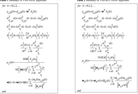
, from Eq. (13). Finally, the entire adaptive algorithm is described by Eqs. (12, 23, 26-28). Table 1 summarizes VSS-NSAF algorithm.

3.2 VSS-SPU-NSAF Algorithm

The filter coefficients update for VSS-SPU-NSAF is introduced: ∑− = + = + 1

0 _{, ( )}2 ) ( , ) ( , ) ( ) ( ) 1 ( N

i _{iF k}

k D i e k F i k F k F k F x x U w w (29)

where U _F(k)=diag

[

μ_j1(k),...,μ_js(k)

]

. Using the

approximation for e_i,D(k) as

) ( , ) ( ~ ) ( , ) (

,D k TiF k F k viD k i

e ≈ x w + and substituting it

into (29), we obtain:

(

)

∑− = + + = + 1

0 _{, ( )} 2

) ( , ) ( ~ ) ( , ) ( , ) ( ) ( ) 1 ( N

i _{i F k}

k D i v k F k T F i k T F i k F k F k F x w x x U w w (30)

Rewrite Eq. (30) as a weight error vector: ∑−

= −

=

+ 1

0 _{, ( )}2 ) ( , ) ( , ) ( ) ( ) 1 ( ~ ~ N

i _{iF k}

k D i v k F i k F F k k F x x U w Q w (31) where: ∑− = − = 1

0 _{( )} 2

, , ) ( , ) ( ) ( N i _K F i T F i k F i k F SL k _x x x U I Q (32) and SL I

is the SL×SL identity matrix. To obtain MSD we can write:

[

~_{( )} 2

] [

~ _{( )} 2

] [

~ _{( )}2

]

)

(k =E k =E _F k +E _F′ k

Λ w w w (33)

where E

⎢⎣

⎡

W~_F′(k) 2

⎥⎦

⎤

are weights that are not selected to update. Therefore:

[

~ _{( 1)} 2

] [

~ _(k)2

]

F k

F′ + = w ′

w

(34)

Combining Eq. (31) and Eq. (33) leads to:

[

]

[ ]

1

[

~ _{( )}2

]

0 2 2 , 2 ) ( ) ( 2 ) ( ~ ) ( ) ( ) ( ~ ) 1 ( k F E N i i x D i v SL k F Tr k F k k T k T F E k ′ + ∑− = + = + Λ w U w Q Q w σ σ (35)

Similar to [15], we assume again that x_i(kN) and

) ( ,D k i

v are zero-mean i.i.d. stationary with variance 2

i

x

σ and 2 ,D i v

σ , r)espectively; ~w (k),x_i(kN), and , )

( ,D k i

v are mutually independent and

1 2 ) ( , ) (

, k i F k ≈SL x_i for SL>> T F i σ x x

.

Therefore, we obtain:

[

]

[ ]

2 ( ) 2 ) ( ) ( 2 1 ) ( )

( _F k

SL N SL SL k F NTr k k T

E I U

U Q Q − + = ⎪⎭ ⎪ ⎬ ⎫ ⎪⎩ ⎪ ⎨ ⎧

(36)

By combining Eq. (35) and Eq. (36), we get:

[ ]

[

]

[

]

[ ]

1

[

~ _{( )}2

]

0 2 2 , 2 ) ( ) ( 2 ) ( ~ ) ( ) ( ~ ) ( 2 2 ) ( ~ 2 ) ( ) ( 2 1 ) 1 ( k F E N i i x D i v SL k F Tr k F k F k T F E SL N k F E SL k F NTr k ′ + ∑− = + + = + Λ

⎪⎭

⎪

⎬

⎫

⎪⎩

⎪

⎨

⎧

w U w U w w U

-σ σ (37)

Taking the first-order partial derivative of Λ(K+1)

with respect to μ_j(k)

(

j=0,_K,SL−1

)

, and setting it to zero for j∈F , we obtain:

[

]

[ ]

1 0

0 2 2 , ) ( 2 ) ( 2 ) ( 2 ~ 2 2 ) ( ) ( 2 2 ) ( ~ ) ( ) 1 ( = ∑− = + − = ∂ + Λ ∂ N i i x D i v k j SL k j w E SL N SL k j N k F E k j K σ σ μ μ μ w (38) Therefore:

[ ]

[

]

∑− = + = 1 0 2 2 , 2 ) ( ~ ) ( 2 ~ ) ( ) ( N i i x D i v k F NE k j w E SL N k j σ σ μ w ₍₃₉₎

To update E

[ ]

w~2_j(k) , the following equation is obtained by taking the mean square of the jth entry in Eq. (31).

[

]

[

]

[ ]

∑− = + + − = +

⎥⎦

⎤

⎢⎣

⎡

1 0 2 2 , 2 ) ( ) ( 2 2 ) ( ~ 2 ) ( ) ( 2 ) ( 2 ~ ) ( 2 1 ) 1 ( 2 ~ N i i x D i v SL k j k F W E SL k j N k j w E k j SL N k j w E σ σ μ μ μ (40)

Using the following assumption as:

[

]

[

]

2

, 2 ) ( ~ 2 ) ( 2

,D k x_iE F k v_{i D}

i e

E ≈σ w +σ ₍₄₁₎

and substituting it into Eq. (40), the following relation is obtained:

[

]

[

]

[ ]

[

]

∑− = + − = + 1 0 2 ) ( 2 , 2 ) ( ) ( 2 ) ( 2 ~ ) ( 2 1 ) 1 ( 2 ~ N i i x k D i e E SL k j k j w E k j SL N k j w E σ μ μ (42)

where E

[

e_i2_,D(k)

]

and 2 i x

σ are estimated according to Eqs. (27) and (28). Table 2 summarizes the VSS-SPU-NSAF algorithm.

4 Computational Complexity

Table 3 shows the number of multiplications, divisions, and comparisons of different adaptive algorithms. The computational complexity of NSAF for each input sampling period is exactly 3M +3NK +1 multiplications and 1 division, where K is the length of the channel filters of the analysis filter bank, M is the number of filter coefficients, and N is the number of subbands. SPU-NSAF needs 2M+SL+3NK+1 multiplications, 1 division, and O(B)+Blog2(S) comparisons when using the heapsort algorithm [16]. The proposed VSS-NSAF needs 5M+8 multiplications and 3 divisions more than conventional NSAF. Using SPU approach in VSS-NSAF leads to the reduction in number of multiplications. The number of multiplications is 7M + SL + 3NK + 8 in this algorithm. The VSS-SPU-NSAF algorithm needs also 4 divisions and O(B) + Blog2(S) comparisons. We have also presented the computational complexity of set membership NSAF (SM-NSAF) [8] and VSS-NSAF [13] in Table 3. The SM-NSAF needs 3M+3NK+1 multiplications, 2 divisions and N comparisons during each iteration which is lower than proposed VSS-NSAF. We will show in simulation results section that the steady-state error of this algorithm is higher than proposed algorithm. The VSS-NSAF in [13] needs 3M + 3NK + 1 multiplications, 3 divisions, 3M+5 additional multiplications and N comparisons. In this algorithm, each subband has the variable step-size. Therefore we have N variable step-size. In the proposed VSS-NSAF algorithm, the number of variable step-size is equal to M. Therefore, the computational complexity is slightly increased. But the proposed VSS-SPU-NSAF reduces the number of multiplications during the adaptation due to the partial update. Furthermore, the convergence speed of the presented VSS-NSAF algorithms is better than SM-NSAF [8] and VSS-NSAF [13].

5 Simulation Results

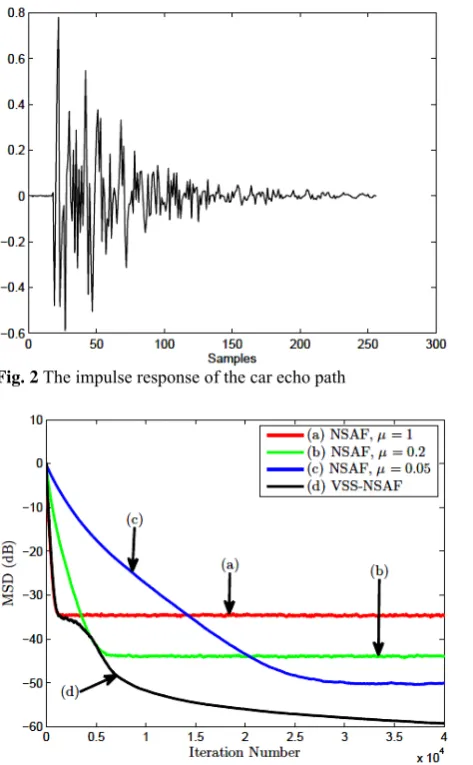
We demonstrate the performance of the proposed algorithms by several computer simulations in a system identification scenario. In the first simulation, we use the real acoustic impulse response with length M = 256 as shown in Fig. 2 [17]. The same length is used for the adaptive filter. The colored Gaussian signal is used for the input signal. The input signal is obtained by filtering a white, zero-mean and unit variance Gaussian random sequence through a second order auto regressive (AR(2)) system with transfer function

2 8 . 0 1 1 . 0 1 1 ) ( ₋ − − − = z z z

T . The filter bank used in NSAF

was the four subband extended lapped transform (ELT) (N = 4) [18]. The white zero-mean Gaussian noise was added to the filter output such that the SNR = 30dB.

In all simulations, we show the normalized MSD,

2 2 ) (

o E

k o E

w

w

w

−

which is evaluated by ensemble

averaging over 20 independent trials. Also, we assume that the noise variance, 2

v

σ , is known a priori [19]. For all simulations we consider λ=0.999. Fig. 3 compares the convergence rate of the NSAF algorithm with the

proposed VSS-NSAF when the real unknown impulse response should be identified. In NSAF, different step sizes (1; 0.2 and 0.05) were chosen. As we can see, the proposed VSS-NSAF has both fast convergence rate and low steady-state MSD features compared with ordinary NSAF. Fig. 4 shows the normalized MSD curves for the proposed VSS-NSAF for

1 ,..., 0 ),

( = −

−

=e j r j j M o

W τ where r(j) is a white

Gaussian random sequence with zero-mean and variance σ_r2 of 0.09. In this case, the impulse response length is M = 200, and the envelope decay rate τ is set

Table 1 Summary of VSS-NSAF algorithm

0,1,2,

( ) ( ) ( )

, ,

2 2 2

ˆ ( ) ˆ ( 1) (1 ) _, ( )

, ,

2 2 2

ˆ ( ) ˆ ( 1) (1 ) ( )

2

2_{( 1) 1 ( )} 2_{( )}

2 ˆ ( ) 2( ) 1 _,

2 ₀ 2

( ) ( )

for k

T e_{i D}k d_{i D} k X k_i

k k e_{i D}k

e_{i D} e_{i D}

k k x kN_i

x_i x_i N

E w k_{j j} k E w k_j

M

k

k N e

j i D

M i

xi NME w k_j k

j

σ λσ λ

σ λσ λ

μ

σ μ

σ

μ =

= −

= − + −

= − + −

⎡ ⎤

⎡ _{+ = −}⎤ ⎡ ⎤₊

⎢ ⎥

⎢ ⎥ ⎢ ⎥

⎣ ⎦ ⎣ ⎦ ⎣ ⎦

− ∑ =

⎡ ⎣ =

K

% %

%

w

2

1 _,

2

( ) ₂

0

( ) ( )

1 _,

( 1) ( ) ( )

2

0 ( )

v

N _{i D}

NE k

i xi k e k

N _{i i D}

k k k

i _i k

end

σ

σ ⎤

⎢ _⎥⎦

−

⎡ _{⎤+ ∑}

⎢ ⎥

⎣ _{⎦ =}

−

+ = + ∑

=

%w

x

w w U

x

Table 2Summary of VSS-SPU-NSAF algorithm

0,1,2,

( ) ( ) ( )

, ,

2 2 2

ˆ ( ) ˆ ( 1) (1 ) _, ( )

, ,

2 2 2

ˆ ( ) ˆ ( 1) (1 ) ( )

2

2_{( 1) 1 ( )} 2_{( )}

2 ˆ ( ) 2( ) 1 _,

2 2

( ) 0

( ) ( )

for k

T e_{i D}k d_{i D}k X k_i

k k e_{i D}k

e_{i D} e_{i D}

k k x kN_i

x_i x_i N

E w k_{j j} k E w k_j

SL k

k N e

j i D

SL i _xi

N SL E k

j

σ λσ λ

σ λσ λ

μ

σ μ

σ

μ =

= −

= − + −

= − + −

⎡ ⎤

⎡ _{+ = −}⎤ ⎡ ⎤₊

⎢ ⎥

⎢ ⎥ ⎢ ⎥

⎣ ⎦ ⎣ ⎦ ⎣ ⎦

− ∑ =

=

K

% %

%

w

( ) 2 1

2 ,

( )

2 0

( ) ( )

1 , ,

( 1) ( ) ( )

2

0 _{( )}

, w k_j

v

N _{i D}

NE _F k i

xi

k e k

N _{i F i D}

k k k

F F F

i _k

i F end

σ

σ

⎡ ⎤

⎢ ⎥

⎣ ⎦

−

⎡ _{⎤+ ∑}

⎢ ⎥

⎣ _{⎦ =}

−

+ = + ∑

=

%w

x

w w U

x

Table 3Computational complexity of the family of VSS-NSAF algorithms

Comparisons Additional

Multiplications Divisions

Multiplications Algorithm

- -

1

1 3 3M+ NK+

NSAF [7]

) ( 2 log )

(B B S

O +

-

1

1 3 2M+SL+ NK+

SPU-NSAF [8]

N

-

2

1 3 3M+ NK+

SM-NSAF[8]

N

5

3M+

3 1

3 3M+ NK+

VSS-NSAF[13]

- 8

5M+

4

NK

M 3

3 +

Proposed VSS-NSAF

) ( 2 log )

(B B S

O +

8 5M+

4

NK SL

M 3

2 + +

Proposed VSS-SPU-NSAF

to 0.04. The simulation results show that for low and large values for the step-size, the performance of NSAF is deviated.

But the VSS-NSAF has both fast convergence speed and low steady-state MSD due to the strategy of variable step-size. In Fig. 5, we presented the results for random unknown impulse response. The parameter M is set to 50. The simulation results show that in the case of random unknown system the performance of VSS-NSAF is deviated, but still, the overall performance is better than ordinary NSAF algorithm. Fig. 6 compares the MSD curves of VSS-NSAF, and VSS-SPU-NSAF algorithms when the real unknown impulse response should be identified. The number of blocks (B) was set to 4 and various values for S were selected. By increasing the parameter S, the performance of VSS-SPU-NSAF will be closed to the VSS-NSAF algorithm. Furthermore, the computational complexity of VSS-SPU-NSAF is lower than VSS-NSAF due to partial updates of filter coefficients.

Fig. 2 The impulse response of the car echo path

Fig. 3 The MSD curves of VSS-NSAF and conventional

NSAF forreal unknown impulse response

Fig. 4 The MSD curves of VSS-NSAF and conventional NSAF for exponential unknown impulse response

Fig. 5 The MSD curves of VSS-NSAF and conventional NSAF for random unknown impulse response

Fig. 6 The MSD curves of VSS-SPU-NSAF with B=4 and

S=2, 3, and 4 for real unknown impulse response

Fig. 7 The MSD curves of SM-NSAF [8], VSS-NSAF [13], and proposed VSS-NSAF for real unknown impulse response

Fig. 7 compares the performance of the proposed algorithm with other VSS-NSAF algorithms in [8], and [13]. In [8], the convergence speed is high during the initial iterations. But the steady-state error is large. In this algorithm, the variable step-size is the same for all the coefficients. The performance of VSS-NSAF in [13] is better than SM-NSAF due to the variable step-size for each subband. As we can see, the proposed VSS-NSAF has better performance than other algorithms in both of convergence speed and steady-state error.

6 Conclusion

In this paper we presented the new variable step-size NSAF algorithm. This algorithm had fast convergence speed and low steady-state MSD compared with ordinary NSAF algorithm. To reduce the computational complexity of VSS-NSAF, the VSS-SPU-NSAF was proposed. We demonstrated the good performance of the presented VSS adaptive algorithms in system identification scenario by several simulation results.

References

[1]. Widrow B. and Stearns S. D., Adaptive Signal Processing. Englewood Cliffs, NJ: Prentice-Hall, 1985.

[2]. Haykin S., Adaptive Filter Theory. NJ: Prentice-Hall, 4th edition, 2002.

[3]. Sayed A. H., Fundamentals of Adaptive Filtering. Wiley, 2003.

[4]. Farhang-Boroujeny B., Adaptive Filters: Theory and Applications. Wiley, 1998.

[5]. Sayed A. H., Adaptive Filters. Wiley, 2008. [6]. de Courville M. and Duhamel P., “Adaptive

filtering in subbands using a weighted criterion”, IEEE Trans. Signal Processing, Vol. 46, pp. 2359-2371, 1998.

[7]. Lee K. A. and Gan W. S., “Improving convergence of the NLMS algorithm using constrained subband updates”, IEEE Signal processing Letters, Vol. 11, pp. 736-739, 2004.

[8]. Abadi M. S. E. and Husoy J. H., “Selective partial update and setmembership subband adaptive filters”, Signal Processing, Vol. 88, pp. 2463-2471, 2008.

[9]. Esfand Abadi M. S., Mehrdad V. and Noroozi M., “A family of selective partial update affine projection adaptive filtering algorithms”, Iranian Journal of Electrical and Electronic Engineering, Vol. 5, No. 3, pp. 159-169, 2009.

[10]. Esfand Abadi M. S. and Nikbakht S., “Image denoising with two-dimensional adaptive filter algorithms”, Iranian Journal of Electrical and Electronic Engineering, Vol. 7, No. 2, pp. 84-105, 2011.

[11]. Shi K. and Ma X., “A variable-step-size nlms algorithm using statistics of channel response”, Signal Processing, Vol. 90, No. 6, pp. 2107-2111, 2010.

[12]. Esfand Abadi M. S., Shafiee M. S. and Abbaszadeh S. A., “A new variable step-size normalized subband adaptive filter algorithm using statistics of channel impulse response”, in Proc. Iranian Conference on Electrical Engineering, Tehran, Iran, May 2012.

[13]. Ni J. and Li F., “A variable step-size matrix normalized subband adaptive filter”, IEEE Trans. Audio, Speech, Language Processing, Vol. 18, pp. 1290-1299, 2010.

[14]. Shynk J. J., “Frequency domain and multirate adaptive filtering”, IEEE Signal Processing Magazine, Vol. 9, pp. 14-37, Jan. 1992.

[15]. Shi K. and Ma X., “A variable-step-size nlms algorithm using statistics of channel response”, Signal Processing, Vol. 90, pp. 2107-2111, 2010. [16]. Knuth D. E., Sorting and Searching vol. 3 of The

Art of Computer Programming. 2nd ed. Reading, MA: Addison-Wesley, 1973.

[17]. Dogancay K. and Tanrikulu O., “Adaptive filtering algorithms with selective partial updates”, Circuits and Systems II: Analog and Digital Signal Processing, IEEE Transactions on, Vol. 48, No. 8, pp. 762-769, 2001.

[18]. Malvar H., “Signal processing with lapped transforms, artech house”, Inc., Norwood, MA, 1992.

[19]. Benesty J., Rey H., Vega L. and Tressens S., “A nonparametric vss nlms algorithm”, Signal Processing Letters, IEEE, Vol. 13, No. 10, pp. 581-584, 2006.

Mohammad Shams Esfand Abadi

was born in Tehran, Iran, on September 18, 1978. He received the B.Sc. degree in Electrical Engineering from Mazandaran University, Mazandaran, Iran and the M.Sc. degree in Electrical Engineering from Tarbiat Modares University, Tehran, Iran in 2000 and 2002, respectively, and the Ph.D.

degree in Biomedical Engineering from Tarbiat Modares University, Tehran, Iran in 2007. Since 2004 he has been with the faculty of Electrical and Computer Engineering, Shahid Rajaee Teacher Training University, Tehran, Iran. His research interests include digital filter theory and adaptive signal processing algorithms.

Mohammad Saeed Shafiee was born

in Estahbanat, Iran on September 18, 1987. He received the B.S. degree in Electrical Engineering from Shahid Rajaee Teacher Training University, Tehran, Iran in 2009. Currently, he is the master student in Shahid Rajaee Teacher Training University, Faculty of Electrical and Computer Engineering, Tehran, Iran. His research interests include digital filter theory and adaptive signal processing algorithms.