Train and Test Tightness of LP Relaxations in
Structured Prediction
Ofer Meshi [email protected]
Ben London [email protected]
Amazon
Adrian Weller [email protected]
University of Cambridge and The Alan Turing Institute
David Sontag [email protected]
MIT CSAIL
Editor:Ivan Titov
Abstract
Structured prediction is used in areas including computer vision and natural language processing to predict structured outputs such as segmentations or parse trees. In these settings, prediction is performed by MAP inference or, equivalently, by solving an integer linear program. Because of the complex scoring functions required to obtain accurate predictions, both learning and inference typically require the use of approximate solvers. We propose a theoretical explanation for the striking observation that approximations based on linear programming (LP) relaxations are often tight (exact) on real-world instances. In particular, we show that learning with LP relaxed inference encourages integrality of training instances, and that this training tightness generalizes to test data.
1. Introduction
Many applications of machine learning can be formulated as prediction problems over structured output spaces (Bakir et al., 2007; Nowozin et al., 2014). In such problems output variables are predicted jointly in order to take into account mutual dependencies between them, such as high-order correlations or structural constraints (e.g., matchings or spanning trees). Unfortunately, the improved expressive power of these models comes at a computational cost, and indeed, exact prediction and learning become NP-hard in general. Despite this worst-case intractability, efficient approximations often achieve very good performance in practice. In particular, one type of approximation which has proved effective in many applications is based on linear programming (LP) relaxation. In this approach the prediction problem is first cast as an integer LP (ILP), and then the integrality constraints are relaxed to obtain a tractable program. In addition to achieving high prediction accuracy, it has been observed that LP relaxations are often tight in practice. That is, the solution to the relaxed program happens to be optimal for the original hard problem (i.e., an integral solution is found). This is particularly surprising since the LPs have complex scoring functions that are not constrained to be from any tractable family. It
c
has been an interesting open question to understand why these real-world instances behave so differently from the theoretical worst case.
This paper addresses this question and aims to provide a theoretical explanation for the frequent tightness of LP relaxations in the context of structured prediction. In particular, we show that an approximate training objective, although designed to produce accurate predictors, also induces tightness of the LP relaxation as a byproduct. Interestingly, our analysis also suggests that exact training may have the opposite effect. To explain tightness on future (i.e., test) instances, we prove several generalization bounds relating average tightness on the training data to expected tightness with respect to the generating distribution. Our bounds imply that if many predictions on training instances are tight, then predictions on test instances are also likely to be tight. Moreover, if predictions on training instances are close tointegral solutions (in terms of L1 distance), then predictions on test instances will likely be similarly close to integral solutions. Our results help to understand previous empirical findings, and to our knowledge provide the first theoretical justification for the widespread success of LP relaxations for structured prediction in settings where the training data is not (algorithmically) separable.
2. Background
In this section we review the formulation of the structured prediction problem, its LP relaxation, and the associated learning problem. Consider a prediction task where the goal is to map a real-valued input vectorxto a discrete output vectory= (y1, . . . , yn). In this work
we focus on a simple class of models based on linear classifiers.1 Particularly, in this setting prediction is performed via a linear discriminant rule: y(x;w) = arg maxy0w>φ(x, y0), where φ(x, y) ∈ Rd is a function mapping input-output pairs to feature vectors, and w ∈ Rd is
the corresponding weight vector. Since the output space is often huge (exponential in n), it will generally be intractable to maximize over all possible outputs.
In many applications the score function has a particular structure. Specifically, we will assume that the score decomposes as a sum of simpler score functions: w>φ(x, y) = P
cw>cφc(x, yc), where yc is an assignment to a (non-exclusive) subset of the variables.
For example, it is common to use such a decomposition that assigns scores to single and pairs of output variables corresponding to nodes and edges of a graph G: w>φ(x, y) = P
i∈V(G)wi>φi(x, yi) +Pij∈E(G)wij>φij(x, yi, yj). Viewing this as a function of y, we can
write the prediction problem as:
max
y
X
c
θc(yc;x, w) , (1)
whereθc(yc;x, w) =wc>φc(x, yc) (we will sometimes omit the dependence onxandwin the
sequel).
Due to its combinatorial nature, the prediction problem is generally NP-hard, but fortunately, efficient approximations have been proposed. Here we will be particularly interested in approximations based on LP relaxations. We begin by formulating prediction
as the following ILP:2 max
µ∈ML
µ∈{0,1}q
X
c X
yc
µc(yc)θc(yc) + X
i X
yi
µi(yi)θi(yi) =θ>µ , (2)
whereML= (
µ≥0 : P
yc\iµc(yc) =µi(yi) ∀c, i∈c, yi
P
yiµi(yi) = 1 ∀i
)
.
Here,µc(yc) is an indicator variable for a factorcand local assignmentyc, andqis the total
number of factor assignments (dimension ofµ). The setMLis known as the local marginal
polytope (Wainwright and Jordan, 2008), and P
yc\iµc(yc) is the marginalization of µc
w.r.t. variable i. First, notice that there is a one-to-one correspondence between feasible µ’s and assignmentsy’s, which is obtained by settingµto indicators over local assignments (yc and yi) consistent with y. Second, while solving ILPs is NP-hard in general, it is
easy to obtain a tractable program by relaxing the integrality constraints (µ ∈ {0,1}q), which may introduce fractional solutions to the LP. This relaxation, sometimes called the
basic linear programming relaxation (Thapper and ˇZivn´y, 2012), is the first level of the Sherali-Adams hierarchy (Sherali and Adams, 1990). This hierarchy provides successively tighter LP relaxations of an ILP. Notice that since the relaxed program is obtained by removing constraints from the original problem, its optimal value upper bounds the ILP optimum. Finally, we note that most of our results below also hold for cases where more complex constraints than those in Eq. (2) are used. For example, some assignments may be forbidden since they do not correspond to feasible global structures such as spanning trees (e.g., Martins et al., 2009b; Koo et al., 2010).
In order to achieve high prediction accuracy, the parametersware learned from training data. In this supervised learning setting, the model is fit to labeled examples{(x(m), y(m))}M
m=1,
where the goodness of fit is measured by a task-specific loss ∆(y(x(m);w), y(m)). We assume that ∆(y, y0)≥0 for ally, y0, and that ∆(y, y) = 0. For example, a commonly used task-loss is the Hamming distance: ∆Hamming(y, y0) = n1Pi1[yi6=y0i].
In the structured SVM (SSVM) framework (Taskar et al., 2003; Tsochantaridis et al., 2004), the empirical risk is upper bounded by a convex surrogate called the structured hinge loss, which yields the training objective:
min w
X
m max
y h
w>φ(x(m), y)−φ(x(m), y(m))+ ∆(y, y(m))i . (3)
For brevity, we have omitted the standard regularization term from Eq. (3), however, all of our results below in sections 4—6 still hold with regularization.3 The objective in Eq. (3)
is a convex function of w and hence can be optimized in various ways. But, notice that the objective includes a maximization over outputsy for each training example. This loss-augmented prediction task needs to be solved repeatedly during training (e.g., to evaluate subgradients), which makes training intractable in general (see also Sontag et al., 2010). Similar to prediction, LP relaxation can be applied to the structured loss (Taskar et al.,
2. For convenience we introduce singleton factorsθi, which could be set to 0 if needed.
2003; Kulesza and Pereira, 2007), which yields the relaxed training objective:
min
w
X
m
max
µ∈ML
h
θm>(µ−µm) +`m>µ
i
, (4)
where θm ∈ Rq is a score vector in which each entry representsw>cφc(x(m), yc) for some c
and yc, and µm is the integral vector corresponding to y(m). Assuming that the task-loss
decomposes as the model score, ∆(y, y0) =P
c∆c(yc, yc0), we define the vector`m∈Rqwith
entries`m,c,yc = ∆c(y
(m)
c , yc) for each valueyc. Notice that ` has the same dimension asµ,
and we can define ∆(y(m), y) =P
c
P
y0
c∆c(y
(m)
c , y0c)µc(yc0) =`m>µ, whereµis the vector of
indicators corresponding toy (i.e.,µc(yc0) =1{yc0 =yc}). With this definition, `generalizes
∆ to anyµ∈ ML.
After reviewing related work in Section 3, we propose a theoretical justification for the observed tightness of LP relaxations for structured prediction. To this end, we make two complementary arguments: in Section 4 we argue that optimizing the relaxed training objective of Eq. (4) also has the effect of encouraging tightness of training instances; then, in sections 5 and 6 we show that tightness generalizes from train to test data.
3. Related Work
Many structured prediction problems can be expressed as ILPs (Roth and Yih, 2005; Martins et al., 2009a; Rush et al., 2010). Despite being NP-hard in general (Roth, 1996; Shimony, 1994), various effective approximations have been proposed. These approximations include search-based methods (Daum´e III et al., 2009; Zhang et al., 2014) and natural LP relaxations to the hard ILPs (Schlesinger, 1976; Koster et al., 1998; Chekuri et al., 2004; Wainwright et al., 2005). Tightness of LP relaxations for special classes of problems has been studied extensively in recent years and has been demonstrated by restricting either the structure of the model or its score function. For example, the pairwise LP relaxation is known to be tight for tree-structured models or for supermodular scores (see, e.g., Wainwright and Jordan, 2008; Thapper and ˇZivn´y, 2012); certain stability conditions guarantee tightness of LP relaxations for Ferromagnetic Potts models (Lang et al., 2018); and the cycle relaxation (for binary pairwise models) is known to be tight both for planar Ising models with no external field (Barahona, 1993) and for almost balanced models (Weller et al., 2016). Hybrid conditions, combining structure and score, by forbidding signed minors have recently been shown to also guarantee tight relaxations (Rowland et al., 2017; Weller, 2016). To facilitate efficient prediction, one could restrict the model class to be tractable. For example, Taskar et al. (2004) learn supermodular scores, and Meshi et al. (2013) learn tree structures.
*0 John1 saw2 a3 movie4 today5 that6 he7 liked8
Important problem in many languages. Problem isNP-Hardfor all but the simplest models.
For example, in
non-projective
dependency parsing
, we found that the
LP relaxation
is exact for over 95%
of
sentences
(Martins et al. ACL ’09, Koo et al., EMNLP ’10)
How often do we exactly solve the problem?
90 92 94 96 98 100
Cze Eng Dan Dut Por Slo Swe Tur
I Percentage of examples where the dual decomposition finds an exact solution.
Language
Percentage of integral solutions
Even when the local LP relaxation is not tight, often still possible to
solve exactly and quickly (e.g., Sontag et al. ‘08, Rush & Collins ‘11)
Figure 1: Percentage of integral solutions for dependency parsing from Koo et al. (2010).be seen in Fig. 1.4 Lacoste-Julien et al. (2006) found that about 80% of test instances had tight LP relaxations in a quadratic assignment formulation for word alignment, with only 0.2% fractional values overall. The same phenomenon has been observed for a multi-label classification task, where test integrality reached 100% (Finley and Joachims, 2008, Table 3).
Learning structured output predictors from labeled data was proposed in various forms by Collins (2002); Taskar et al. (2003); Tsochantaridis et al. (2004). These formulations generalize training methods for binary classifiers, such as the Perceptron algorithm and support vector machines (SVMs), to the case of structured outputs. The learning algo-rithms repeatedly perform prediction, necessitating the use of approximate inference within training as well as at test time. A common approach, introduced right at the inception of structured SVMs by Taskar et al. (2003), is to use LP relaxations for this purpose.
The closest work to ours is by Kulesza and Pereira (2007), which showed that not all approximations are equally good, and that it is important to match the inference algorithms used at train and test time. The authors defined the concept of algorithmic separability which refers to the case where an approximate inference algorithm achieves zero loss on a data set. The authors studied the use of LP relaxations for structured learning, giving generalization bounds for the true risk of LP-based prediction. However, since the generalization bounds in Kulesza and Pereira (2007) are focused on prediction
accuracy, the only settings in which tightness on test instances can be guaranteed are when the training data is algorithmically separable, which is seldom the case in real-world structured prediction tasks (the models are far from perfect). In contrast, our paper’s main result (Theorem 1), guarantees that the expected fraction of test instances for which an LP relaxation is tight is close to that which was achieved on training data. This then allows us to talk about the generalization of computation. For example, suppose one uses LP relaxation-based algorithms that iteratively tighten the relaxation, such as Sontag and Jaakkola (2008); Sontag et al. (2008), and observes that 20% of the instances in the training data are integral using the basic relaxation and that after tightening the remaining 80% are now integral too. Our generalization bound then guarantees that approximately the same ratio will hold at test time (assuming sufficient training data).
Finley and Joachims (2008) also studied the effect of various approximate inference methods in the context of structured prediction. Their theoretical and empirical results support the superiority of LP relaxations in this setting. Martins et al. (2009b) established conditions which guarantee algorithmic separability for LP relaxed training, and derived risk bounds for a learning algorithm which uses a combination of exact and relaxed inference.
Finally, Globerson et al. (2015) recently studied the performance of structured predictors for 2D grid graphs with binary labels from an information-theoretic perspective. They proved lower bounds on the minimum achievable expected Hamming error in this setting, and proposed a polynomial-time algorithm that achieves this error. Our work is different since we focus on LP relaxations as an approximation algorithm, we handle a general form of the problem without making any assumptions on the model or error measure (except score decomposition), and we concentrate solely on the computational aspects while ignoring any accuracy concerns.
4. Tightness at Training
In this section we show that the relaxed training objective in Eq. (4), although designed to achieve high accuracy, also induces tightness of the underlying LP relaxation. In fact, although we focus here on the basic LP relaxation (first-level), the results below hold for higher-level LP relaxations as well.5
In order to simplify notation we focus on a single training instance and drop the index m. Denote the solutions to the relaxed and integer LPs as:
µL∈arg max µ∈ML
θ>µ µI∈arg max µ∈ML
µ∈{0,1}q
θ>µ , (5)
respectively. Also, let µT be the integral vector corresponding to the ground-truth output
y(m). Now consider the following decomposition: θ>(µL−µT)
relaxed-hinge
=θ>(µL−µI) integrality gap
+θ>(µI−µT) exact-hinge
(6)
This equality states that the difference in scores between the relaxed optimum and ground-truth (relaxed-hinge) can be written as a sum of the integrality gap and the difference in scores between the exact optimum and the ground-truth (exact-hinge); notice that all three terms are non-negative. This simple decomposition has several interesting implications.
First, we can immediately derive the following bound on the integrality gap:
θ>(µL−µI) =θ>(µL−µT)−θ>(µI −µT) (7)
≤θ>(µL−µT) (8)
≤θ>(µL−µT) +`>µL (9)
≤ max
µ∈ML
θ>(µ−µT) +`>µ, (10)
where Eq. (10) is precisely the relaxed training objective from Eq. (4). Therefore, optimizing the approximate training objective of Eq. (4) minimizes an upper bound on the integrality
gap. Hence, driving down the approximate objective may also reduce the integrality gap of training instances, although in Section 4.1 we also study cases where loose bounds can lead to non-zero integrality gap. One case where the integrality gap becomes zero is when the data is algorithmically separable (i.e., µL =µT, so Eq. (8) equals 0). In this case the
relaxed-hinge term vanishes (the exact-hinge must also vanish), and training integrality is assured.
Second, Eq. (6) holds for any integral µ, and not just the ground-truth µT. In other
words, the only property of µT used here is its integrality. Indeed, in Section 7 we verify
empirically that training a model usingrandom labels still attains the same level of tightness as training with the ground-truth labels.6 On the other hand, accuracy drops drastically, as expected. This analysis suggests that tightness is not coupled with accuracy of the predictor. Finley and Joachims (2008) explained tightness of LP relaxations by noting that fractional solutions always incur a loss during training. Our analysis suggests an alternative explanation, emphasizing the difference in scores (Eq. (7)) rather than the loss, and decoupling tightness from accuracy.
Third, the results above still hold in the presence of global constraints. Often such constraints can be expressed as linear inequalities, so in this case the local polytope ML
can be redefined by adding these constraints to those in Eq. (2) to form a tighter polytope. In particular, Eq. (8) holds since µT satisfies the global constraints.
Finally, we do not make any assumption here about the form of the model scores θ. Therefore, these results apply more generally, even when factor scores are obtained from non-linear functions of the inputs, such as deep neural networks (e.g., Chen et al., 2015).
4.1. When Relaxed Training is Better than Exact Training
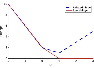
Unfortunately, the bound in Eq. (10) might sometimes be loose. Indeed, to get the bound we have discarded the exact-hinge term (Eq. (8)), added the task-loss (Eq. (9)), and maximized the loss-augmented objective (Eq. (10)). At the same time, Eq. (7) provides a precise characterization of the integrality gap. Specifically, the gap is determined by the difference between the relaxed-hinge and the exact-hinge terms. This implies that even when the relaxed-hinge is not zero, a small integrality gap can still be attained if the exact-hinge is also large. In fact, the only way to get a large integrality gap is by setting the exact-hinge much smaller than the relaxed-hinge. But when can this happen? As we now show, it is less likely to happen when training with relaxed inference than when training with exact inference.
A key point is that the relaxed and exact hinge terms are upper bounded by the relaxed and exacttraining objectivesrespectively (the latter additionally depend on the task loss ∆). Therefore, minimizing the training objective will also likely reduce the corresponding hinge term (this is also demonstrated empirically in Section 7). Using this insight, we observe that relaxed training reduces the relaxed-hinge term without directly reducing the exact-hinge term, and thereby induces a small integrality gap. On the other hand, this also suggests that exact training may actually increase the integrality gap, since it reduces the exact-hinge without also reducing directly the relaxed-exact-hinge term. This finding is consistent with previous empirical evidence. Specifically, Martins et al. (2009b, Table 2) showed that on
w
-2 -1 0 1 2 3
Hinge
0 2 4 6 8 10
Relaxed hinge Exact hinge
Figure 2: Exact- and relaxed- hinge (see Eq. (6)) as a function ofwfor the learning scenario in Section 4.1.
a dependency parsing problem, training with the relaxed objective achieved 92.9% integral solutions, while exact training achieved only 83.5% integral solutions. An even stronger effect was observed by Finley and Joachims (2008, Table 3) for multi-label classification, where relaxed training resulted in 99.6% integral instances, with exact training attaining only 17.7% (‘Yeast’ dataset).
In Section 7 we provide further empirical support for our explanation, however, we next show its possible limitation by providing a counter-example. The counter-example demonstrates that despite training with a relaxed objective, the exact-hinge can in some cases actually besubstantially smallerthan the relaxed-hinge, leading to a loose relaxation. Although this illustrates the limitations of the explanation above, we point out that the corresponding learning task is far from natural.
We construct a learning scenario where relaxed training obtains zero exact-hinge and non-zero relaxed-hinge, so the relaxation is not tight. Consider a model where x ∈ R3,
y∈ {0,1}3, and the prediction is given by: y(x;w) = arg max
y
x1y1+x2y2+x3y3+w[1{y16=y2}+1{y16=y3}+1{y26=y3}]
. (11)
The corresponding LP relaxation is then:
max
µ∈ML
x1µ1(1) +x2µ2(1) +x3µ3(1) (12)
+w[µ12(01) +µ12(10) +µ13(01) +µ13(10) +µ23(01) +µ23(10)]
.
Next, we construct a training set where the first instance is: x(1) = (2,2,2), y(1)= (1,1,0),
and the second is: x(2) = (0,0,0), y(2)= (1,1,0). Fig. 2 shows the relaxed and exact losses as a function of w, obtained by plugging Eq. (11) and Eq. (12) in Eq. (3) and Eq. (4), respectively.7 Observe thatw= 1 minimizes the relaxed objective (Eq. (4)). However, with
this weight vector the relaxed-hinge for the second instance (x(2), y(2)) is equal to 1, while the exact-hinge for this instance is 0 (the data is separable with w = 1). Consequently, there is an integrality gap of 1 for the second instance, and the relaxation is loose (the first
ML
Figure 3: Illustration of the local marginal polytopeML, with its vertices partitioned into
integral verticesVI (blue), and fractional verticesVF (red).
instance is actually tight). Notice that in this data the same output corresponds to two very different inputs.
5. Generalization of Tightness
Our argument in Section 4 concerns only the tightness of train instances. However, the empirical evidence discussed above pertains to test data. To bridge this gap, in this section we prove a generalization bound which shows that train tightness implies test tightness.
We first define a loss function which measures the lack of integrality (or, fractionality) of the LP solution for a given instance. To this end, we consider the discrete set of vertices
of the local polytope ML (excluding its convex hull), denoting by VI and VF the sets of
fully-integral and non-integral (i.e., fractional) vertices,8 respectively (so VI∩ VF =∅, and VI ∪ VF consists of all vertices of ML);9 see Fig. 3. Considering only vertices does not
reduce generality, since the solution to a linear program is always at a vertex. Next, let
I∗(w, x),max
µ∈VI
θ(x;w)>µ and F∗(w, x), max
µ∈VF
θ(x;w)>µ (13)
denote the respective best integral and fractional scores. By convention, we setF∗(w, x),
−∞ whenever VF =∅. The fractionality of inference with (w, x) can be measured by the
quantity
D(w, x),F∗(w, x)−I∗(w, x). (14)
Observe thatD(w, x)>0 whenever the LP has a fractional solution that is better than the integral solution. We can now define the integrality loss,
L0(w, x),
(
1 D(w, x)>0
0 otherwise . (15)
8. It is enough that one coordinate is fractional to belong toVF.
9. We assume that all feasible integral solutions are vertices ofML, which is the case for the type of
This loss function equals 1 if and only if the optimal fractional solution has a (strictly) higher score than the optimal integral solution. The loss will be 0 whenever the non-integral and integral optima are equal—that is, for our purpose we consider the relaxation to be tight in this case. The expected integrality loss measures the probability of obtaining a fractional LP solution (over draws of an input, x). Note that this loss ignores the ground truth assignment.
To support our generalization analysis, we define a related loss function, which we call the integrality ramp loss. For a predetermined margin parameter, γ, the integrality ramp loss is given by
Lγ(w, x),
1 D(w, x)>0
1 +D(w, x)/γ −γ < D(w, x)≤0
0 D(w, x)≤ −γ
. (16)
Importantly, the integrality ramp loss upper-bounds the integrality loss. For the ramp loss to be zero, the best integral solution has to be better than the best fractional solution by a margin of at leastγ, which is a stronger requirement than mere tightness. In Appendix A we give examples of models that are guaranteed to satisfy this requirement, and in Section 7 we also show this often happens in practice.
We point out that both L0(w, x) and Lγ(w, x) are generally hard to compute, a point
which we address in Section 6. For the time being, we are only interested in proving that tightness is a generalizing property, so we will not worry about computational efficiency.
We are now ready to state the main theorem of this section, a generalization bound for tightness. Our proof (deferred to Appendix B.1) uses a PAC-Bayesian analysis, similar to London et al. (2016), though the main result is stated for a deterministic predictor.
Theorem 1. Let D denote a distribution over X. Let φ : X × Y → Rd denote a feature mapping such that supx,ykφ(x, y)k2≤B <∞. Then, for any γ >0, δ ∈(0,1) andm≥1, with probability at least 1−δ over draws of (x(1), . . . , x(m)) ∈ Xm, according toDm, every weight vector, w, withkwk2 ≤R <∞, satisfies
E
x∼D[L0(w, x)]≤
1 m
m
X
i=1
Lγ(w, x(i)) +
8
m + 2
s
dln(mBR/γ) + ln2δ
2m . (17)
Theorem 1 shows that if we observe high integrality (equivalently, low fractionality) on a finite sample of training data, then it is likely that integrality of test data will not be much lower, provided sufficient number of samples. It is worth noting that, though we focus on linear models to simplify our presentation, it is possible to extend this result to accommodate non-linear models (e.g., scores θ computed by a deep neural network), provided some assumptions are made on the smoothness of the model and loss.
As the following corollary states, Theorem 1 actually applies more generally to any two disjoint sets of vertices, and is not limited toVI and VF.
Corollary 1. Let Vα be any set of vertices of ML with at mostα fractional values (where
For example, we can setVα to be any set of vertices with at most 10% fractional values,
and ¯Vαto be the rest of the vertices ofML. This gives a different meaning to the integrality
loss, but the rest of our analysis holds unchanged. Consequently, our generalization result implies that it is likely to observe a similar portion of instances with at most 10% fractional values at test time as we did at training.
Moreover, Theorem 1 also holds in the presence of global constraints (e.g., spanning tree constraints). As mentioned in Section 4, the polytope ML is replaced by its intersection
with the global constraints polytope, but the rest of our derivation remains unchanged. Note that the loss function in Eq. (15) does not measure the actual number of fractional values, nor theirdistance to integrality. In Section 6, we analyze a notion of tightness that accounts for the L1 distance to integrality.
Compared to the generalization bound of Kulesza and Pereira (2007), our bounds only consider the tightness of a prediction, ignoring label errors. Thus, for example, if learning happens to settle on a set of parameters in a tractable regime (e.g., supermodular potentials or stable instances (Makarychev et al., 2014)) for which the LP relaxation is tight for most training instances, our generalization bound guarantees that with high probability the LP relaxation will also be tight on most test instances. In contrast, in Kulesza and Pereira (2007), tightness on test instances can only be guaranteed when the training data is algorithmically separable (i.e., LP-relaxed inference predicts perfectly).
5.1. γ-Tight Relaxations
In this section we study the stronger notion of tightness required by our surrogate fraction-ality loss (Eq. (16)), and show examples of models that satisfy it.
Definition 1. An LP relaxation is calledγ-tight ifI∗(w, x)≥F∗(w, x) +γ (soLγ(w, x) =
0). That is, the best integral value is larger than the best non-integral value by at leastγ.10 We focus on binary pairwise models and show two cases where the model is guaranteed to be γ-tight. Proofs are provided in Appendix A. Our first example involves balanced
models, which are binary pairwise models that have supermodular scores, or can be made supermodular by “flipping” a subset of the variables (for more details, see Appendix A).
Proposition 1. A balanced model with a unique optimum is (α/2)-tight, where α is the difference between the best and second-best (integral) solutions.
This result is of particular interest when learning structured predictors where the edge scores depend on the input. Whereas one could learn supermodular models by enforcing linear inequalities (Taskar et al., 2004), we know of no tractable means of ensuring the model is balanced. Instead, one could learn over the full space of models using LP relaxation. If the learned models are balanced on the training data, Proposition 1 together with Theorem 1 tell us that the LP relaxation is likely to be tight on test data as well.
Our second example regards models with singleton scores that are much stronger than the pairwise scores. Consider a binary pairwise model11 in minimal representation, where ¯
θi are node scores and ¯θij are edge scores in this representation (see Appendix A for full
10. Notice that scaling upθ(w, x) will also increaseγ, but our bound in Eq. (17) also grows with the norm ofθ(w, x) (via the termBR). Therefore, we assume here thatkθ(w, x)k2 is bounded.
details). Further, for each variablei, define the set of neighbors withattractiveedgesNi+=
{j∈Ni|θ¯ij >0}, and the set of neighbors with repulsive edges Ni−={j∈Ni|θ¯ij <0}.
Proposition 2. If all variables satisfy the condition:
¯ θi ≥ −
X
j∈Ni−
¯
θij +β, or θ¯i≤ −
X
j∈Ni+
¯ θij−β
for some β >0, then the model is (β/2)-tight.
Finally, we point out that in both of the examples above, the conditions can be verified efficiently and if they hold, the value ofγ can be computed efficiently.
6. Analysis of the Integrality Distance
For structured prediction, the maximizer, µL, is often more important than the maximum
value, θ>µL. That is, we do not really care whether the optimum of the relaxed problem
equals that of the integral one; we just want relaxed inference to yield the optimal integral assignment—or, lacking that, an assignment that is “close to” the optimal integral one. If we assume that the relaxed problem has a unique solution, then an integrality gap of zero implies that the assignments are the same. However, lacking this assumption, there may be multiple, disparate solutions, so the assignments may differ. In general, it is difficult to characterize the distance between relaxed and exact assignments as a function of a nonzero integrality gap.
Thus, in addition to studying the integrality gap, we are also interested in what we will call the integrality distance, defined as kµL−µIk1, which is the Manhattan distance
between the maximizers of the relaxed and exact programs. The integrality distance is conceptually similar topersistence (see Wainwright and Jordan, 2008 for definition) in that a persistent fractional solution will have a subset of variables with zero integrality distance. The integrality distance is also related to the integrality gap, although the distance could sometimes be more useful: when the integrality distance is small, the relaxed solution is close to the exact solution, which is what we may ultimately care about; moreover, when the integrality distance is zero, the integrality gap must also be zero, regardless of whether we assume uniqueness.
6.1. Structured Loss Functions
We will focus on the integrality distance of the singleton (i.e., node) marginals, denoted µu,(µi)ni=1, since they are sufficient for decoding a labeling, y. Let
D1(µ, µ0),
1 2n
µu−µ0u
1 (18)
denote the normalized Manhattan distance. When both inputs are integral,D1 is equivalent
to the normalized Hamming distance.
Given a model, w, an input, x, and an assignment,µ, let
L1(w, x, µ),D1(µ, µL(x;w)) (19)
denote the L1 loss. This loss function is a generalization of the Hamming loss, which is
commonly used to measure the prediction error of exact inference. If the third argument is a reference (i.e., “ground truth”) labeling,µT, then L1(w, x, µT) measures the prediction
error of approximate inference. However, if the third argument is the exact, integral MAP state, µI, then L1(w, x, µI) is the normalized integrality distance. This latter quantity is
what we will focus on upper-bounding. Let
Lh(w, x, µ), max µ0∈M
L
D1(µ, µ0) +θ> µ0−µ
. (20)
denote a loss function commonly referred to as the (relaxed) structured hinge loss. This loss is minimized whenµscores higher than all alternate assignments,µ0, by a margin that is at least D1(µ, µ0). Note that when µ is the exact MAP state, the structured hinge loss
computes aloss-augmented integrality gap, using Manhattan distance for loss augmentation (see Eq. (4)).
A related loss function is the (relaxed) structured ramp loss,
Lr(w, x, µ), max µ0∈M
L
D1(µ, µ0) +θ> µ0−µL(x;w)
, (21)
which can be considered a normalized version of the hinge loss. Lr is bounded by [0,1],
whereas Lh might be unbounded (depending on the features and weights).
The hinge loss is often used in max-margin training, since it is convex in w. The ramp loss is not convex in w, but it is bounded, Lipschitz, and has a convenient relationship to the L1 (or Hamming) and hinge losses:
L1(w, x, µ)≤ Lr(w, x, µ)≤ Lh(w, x, µ). (22)
Thus, the ramp loss is often used as an analytical tool to derive generalization bounds, such as those that follow.
6.2. Generalization Bound
Theorem 2. Let D denote a distribution over X. Let φ : X × Y → Rd denote a feature mapping such that supx,ykφ(x, y)k2 ≤B <∞; andµI is defined in Eq. (5). Then, for any
δ ∈ (0,1) and m ≥1, with probability at least 1−δ over draws of (x(1), . . . , x(m)) ∈ Xm, according to Dm, every weight vector, w, withkwk2≤R <∞, satisfies
E
x∼D[L1(w, x, µI)]≤
1 m
m
X
i=1
Lr(w, x(i), µ(Ii)) +
8
m + 2
s
dln(mBR) + ln2δ
2m . (23)
Further, Eq. (23) holds when Lr is replaced with Lh.
Theorem 2 says that the integrality distance on the training set generalizes to future examples. More precisely, the expected integrality distance on a random instance is upper-bounded by the average integrality ramp (or hinge) loss on the training set, plus two terms that vanish as the number of training examples grows. Thus, the more training data we have, the better we can estimate the expected integrality distance.
Remark 1. There is nothing special about µI to Theorem 2. Indeed, we could use any
integral assignment as a reference labeling for the loss functions and the proof would be the same. For example, we could replaceµIwithµT (a ground truth labeling) and obtain a risk
bound for learning with approximate inference, which is a well-studied topic (e.g., Kulesza and Pereira, 2007; London et al., 2016).
6.3. Relationship to Max-Margin Training
In practice, computing the integrality loss is generally infeasible, since it requires exact inference. Therefore, the upper bounds in Theorems 1 and 2 cannot be evaluated. However, the empirical relaxed hinge loss with respect to the ground truth labels can be evaluated efficiently. In this section, we show how minimizing this quantity actually minimizes the integrality distance. That is, max-margin training with approximate inference—which is commonly used anyway to learn graphical models—reduces not only the prediction error, but also the inference approximation error.
The key insight that enables this result comes from the following technical lemma.
Lemma 1. For any w and x, if µT is the reference (ground truth) labeling of x and µI is the exact MAP state under w, then
Lh(w, x, µI) ≤ 2Lh(w, x, µT), (24)
meaning the integrality hinge loss is at most twice the hinge loss with respect to the true labeling.
Proof First, we decompose the integrality hinge loss as follows:
Lh(w, x, µI) = max µ∈ML
D1(µI, µ) +θ>(µ−µI) ≤ max
µ∈ML
D1(µI, µ) +θ>(µ−µT) ≤D1(µI, µT) + max
µ∈ML
D1(µT, µ) +θ>(µ−µT)
The second term on the right-hand side is the hinge loss of the approximate predictor with respect to the true labeling, which can be evaluated efficiently. The first term on the right-hand side is the Hamming loss of exact inference, which cannot be evaluated efficiently. However, this latter quantity can be upper-bounded as follows:
D1(µI, µT)≤max
µ∈MD1(µ, µT) +θ >(µ
−µT)
≤ max
µ∈ML
D1(µ, µT) +θ>(µ−µT)
=Lh(w, x, µT). (26)
Combining Eq. (25) and (26) completes the proof.
Note that Lemma 1 also yields an upper bound on the integrality ramp loss, since it is upper-hounded by the integrality hinge loss.
Using Lemma 1, we thus obtain the following corollary of Theorem 2.
Corollary 2. Let Ddenote a distribution overX × Y. Letφ:X × Y →Rddenote a feature mapping such that supx,ykφ(x, y)k2 ≤B < ∞. Then, for any δ ∈ (0,1) and m ≥1, with probability at least 1−δ over draws of (x(1), y(1), . . . , x(m), y(m))∈(X × Y)m, according to Dm, every weight vector, w, withkwk2 ≤R <∞, satisfies
E x∼D
[L1(w, x, µI)]≤
2 m
m
X
i=1
Lh(w, x(i), µ(Ti)) +
8
m + 2
s
dln(mBR) + ln2δ
2m , (27)
where µ(Ti) denotes the integral vector corresponding to the ground-truth labelingy(i).
Corollary 2 says that max-margin training with relaxed inference directly minimizes the integrality distance on future examples. Importantly, if the constantsB and R are known, then this bound can be efficiently evaluated from training data. It is worth noting that Corollary 2 actually holds for any integral assignment, not just the ground truth labels. Nonetheless, we feel the bound is more insightful when stated with respect to the ground truth labels, which are given in the learning setup. In this case D is defined as a joint
distribution over X and Y, and the bound holds with high probability over draws of both inputs and labels. It is also worth noting that Corollary 2 holds in the presence of global constraints—provided the ground truth (or whichever integral assignments are used) are in the feasible set.
6.4. Decoding a Solution
When the solution to an LP relaxation is fractional, we often round the solution to an integral assignment. Rounding schemes have been studied extensively (e.g., Raghavan and Tompson, 1987; Kleinberg and Tardos, 2002; Chekuri et al., 2004; Ravikumar et al., 2010). Arguably, the simplest method is to select the local assignments µi(yi) with the highest
values. One question that arises is how far the rounding, denoted µR(x;w), is from the
exact solution; once this relationship is determined, one can apply our prior generalization analysis to the rounding. It turns out that the distance fromµRtoµIcan be upper-bounded
0 50 100 150 200 0
0.5 1
Relaxed Training
Relaxed−hinge Exact−hinge Relaxed SSVM obj Exact SSVM obj
0 50 100 150 200 0
0.5 1
Training epochs
Train tightness Test tightness Relaxed test F1
Exact test F1
0 50 100 150 200 250
0 0.5 1
1.5 Exact Training
Training epochs
0 50 100 150 200 250
0 0.5 1
−0.4 −0.2 0 0
100 200
Relaxed Training
−0.4 −0.2 0 0
100 200
Exact Training
I*−F*
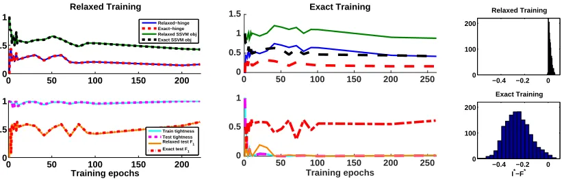
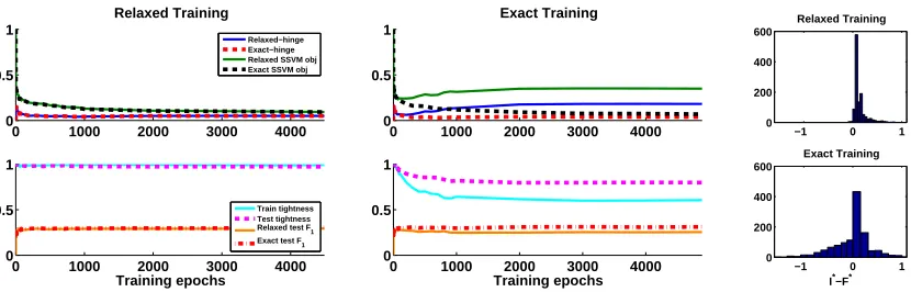
Figure 4: Training with the ‘Yeast’ multi-label classification dataset. Various quantities of interest are shown as a function of training iterations. (Left) Training with LP relaxation. (Middle) Training with ILP. (Right) Integrality margin (bin widths are scaled differently).
Lemma 2. Suppose that every output variable has the same domain—i.e.,Y1 =Y2=. . .=
Yn—and that each domain has size k. IfµR(x;w)is the rounding of the fractional solution,
µL(x;w), then
D1(µR, µI) ≤ k D1(µL, µI). (28)
Proof Consider any output variable. If the fractional solution assigns the majority of the local belief to the “correct” label (i.e., the label chosen by exact inference), then the rounding of that variable will be exact. However, if the fractional solution puts most of the local belief on an “incorrect” label, then the rounding of that variable will haveD1 distance
1 from the correct label. Since the incorrect label must have had a fractional value of at least 1/k, it follows that the fractional solution hasD1distance at least 1/k, which is no less
than 1/kthat of the rounding. Applying this logic to every variable completes the proof.
Lemma 2 can be combined with Corollary 2 to generate bounds on the expected inte-grality distance of rounding; the bound simply scales byk.
7. Experiments
In this section we present some numerical results to support our theoretical analysis. We run experiments for a multi-label classification task and an image segmentation task. For training we have implemented the block-coordinate Frank-Wolfe algorithm for structured SVM (Lacoste-Julien et al., 2013), using GLPK as the LP solver. We use a standard L2
regularizer, chosen via cross-validation.
7.1. Multi-Label Classification
0 100 200 300 400 500 0
0.5 1
Relaxed Training
Relaxed−hinge Exact−hinge Relaxed SSVM obj Exact SSVM obj
0 100 200 300 400 500 0
0.5 1
Training epochs
Train tightness Test tightness Relaxed test F 1 Exact test F
1
0 50 100 150 200 250 300
0 0.5
1 Exact Training
Training epochs
0 50 100 150 200 250 300
0 0.5 1
−0.20 0 0.2 0.4 0.6 100
200 300
Relaxed Training
−0.20 0 0.2 0.4 0.6 100
200 300
Exact Training
I*−F*
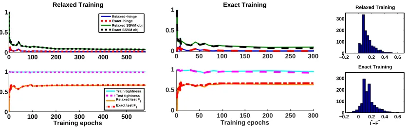
Figure 5: Training with the ‘Scene’ multi-label classification dataset. Various quantities of interest are shown as a function of training iterations. (Left) Training with LP relaxation. (Middle) Training with ILP. (Right) Integrality margin.
singleton and pairwise factors forming a fully connected graph over the labels, and the task loss is the normalized Hamming distance.
Fig. 4 shows relaxed and exact training iterations for the ‘Yeast’ dataset (14 labels). We plot the relaxed and exact hinge terms (Eq. (6)), the exact and relaxed SSVM training objectives12 (Eq. (3) and Eq. (4), respectively), fraction of train and test instances having
integral solutions, as well as test accuracy (measured byF1 score). We use a simple scheme
to round fractional solutions found with relaxed inference. First, we note that the relaxed-hinge values are nicely correlated with the relaxed training objective, and likewise the exact-hinge is correlated with the exact objective (left and middle, top). Second, observe that with relaxed training, the relaxed-hinge and the exact-hinge are very close (left, top), so the integrality gap, given by their difference, remains small (almost 0 here). On the other hand, with exact training there is a large integrality gap (middle, top). Indeed, we can see that the percentage of integral solutions is almost 100% for relaxed training (left, bottom), and close to 0% with exact training (middle, bottom). In Fig. 4 (right) we also show histograms of the difference between the optimal integral and fractional values, i.e., the integrality margin (I∗(w, x)−F∗(w, x)), under the final learnedw for all training instances. It can be seen that with relaxed training this margin is positive (although small), while exact training results in larger negative values. Finally, we note that train and test integrality levels are very close to each other, almost indistinguishable (left and middle, bottom), which provides empirical support to our generalization result from Section 5.
We next train a model using random labels (with similar label counts as the true data). In this setting the learned model obtains 100% tight training instances (not shown), which supports our observation that any integral point can be used in place of the ground-truth, and that accuracy is not important for tightness. Finally, in order to verify that tightness is not coincidental, we test the tightness of the relaxation induced by a random weight vector w. We find that random models are never tight (in 20 trials), which shows that tightness of the relaxation does not come by chance.
0 200 400 600 800 1000 0
1 2 3x 10
4 Relaxed Training
Relaxed−hinge Exact−hinge Relaxed SSVM obj Exact SSVM obj
0 200 400 600 800 1000 0
0.5 1
Training epochs
Train tightness Test tightness Relaxed test accuracy Exact test accuracy
0 200 400 600 800 1000 0
1 2 3x 10
4 Exact Training
0 200 400 600 800 1000 0
0.5 1
Training epochs
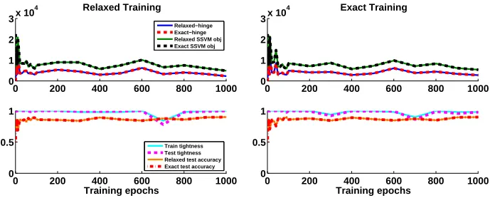
Figure 6: Training for foreground-background segmentation with the Weizmann Horse dataset. Various quantities of interest are shown as a function of training iterations. (Left) Training with LP relaxation. (Right) Training with ILP.
We now proceed to perform experiments on the ‘Scene’ dataset (6 labels). The results, in Fig. 5, differ from the ‘Yeast’ results in case of exact training (middle). Specifically, we observe that in this case the relaxed-hinge and exact-hinge are close in value (middle, top), as for relaxed training (left, top). As a consequence, the integrality gap is very small and the relaxation is tight for almost all train (and test) instances. These results illustrate that sometimes optimizing the exact objective can reduce the relaxed objective (and relaxed-hinge) as well. Further, in this setting we observe a larger integrality margin (right), namely the integral optimum is strictly better than the fractional one.
We conjecture that the LP instances are easy in this case due to the dominance of the singleton scores.13 Specifically, the features provide a strong signal which allows label assignment to be decided mostly based on the local score, with little influence coming from the pairwise terms. To test this conjecture we inject Gaussian noise into the input features, forcing the model to rely more on the pairwise interactions. We find that with the noisy singleton scores the results are indeed more similar to the ‘Yeast’ dataset, where a large integrality gap is observed and fewer instances are tight (see Appendix C in the supplement).
7.2. Image Segmentation
Finally, we conduct experiments on a foreground-background segmentation problem using the Weizmann Horse dataset (Borenstein et al., 2004). The data consists of 328 images, of which we use the first 50 for training and the rest for testing. Here a binary output variable is assigned to each pixel, and there are ∼ 58K variables per image on average. We extract singleton and pairwise features as described in Domke (2013). Fig. 6 shows the same quantities as in the multi-label setting, except for the accuracy measure—here we compute the percentage of correctly classified pixels rather thanF1. We observe a very
similar behavior to that of the ‘Scene’ multi-label dataset (Fig. 5). Specifically, both relaxed and exact training produce a small integrality gap and high percentage of tight instances.
Unlike the ‘Scene’ dataset, here only 1.2% of variables satisfy the condition in Proposition 2 (using LP training). In all of our experiments the learned model scores were never balanced (Proposition 1), although for the segmentation problem we believe the models learned are close to balanced, both for relaxed and exact training.
8. Conclusion
In this paper we present a theoretical analysis of the tightness of LP relaxations often ob-served in structured prediction applications. Our analysis is based on a careful examination of the integrality gap, the integrality distance, and their relation to the training objective. It shows how training with LP relaxations, although designed with accuracy considerations in mind, also induces tightness of the relaxation. Our derivation also suggests that exact training may sometimes have the opposite effect, increasing the integrality gap.
To explain tightness at test time, we show that tightness generalizes in the following two senses: first, if most training predictions are integral, then most test instances will also be integral; secondly, if training predictions are on average “close to” integral, then test predictions will be similarly close to integral in expectation.
Acknowledgments
Appendix A. γ-Tight LP Relaxations
In this section we provide full derivations for the results in Section 5.1. We make extensive use of the results in Weller et al. (2016), some of which are restated here for completeness. We start by defining a model in minimal representation, which will be convenient for the derivations that follow. Specifically, in the case of binary variables (yi ∈ {0,1}) with pairwise
factors, we define a value ηi for each variable, and a value ηij for each pair. The mapping
between the over-complete vector µ and the minimal vector η is as follows. For singleton factors, we have:
µi =
1−ηi
ηi
Similarly, for the pairwise factors, we have:
µij =
1 +ηij−ηi−ηj ηj−ηij ,
ηi−ηij ηij
The corresponding mapping to minimal parameters is then:
¯
θi =θi(1)−θi(0) +
X
j∈Ni
(θij(1,0)−θij(0,0))
¯
θij =θij(1,1) +θij(0,0)−θij(0,1)−θij(1,0)
In this representation, the LP relaxation is given by (up to constants):
max
η∈L f(η) := n
X
i=1
¯ θiηi+
X
ij∈E
¯ θijηij
whereL is the appropriate transformation ofML to the equivalent reduced space ofη:
0 ≤ηi ≤1
max(0, ηi+ηj−1) ≤ηij ≤min(ηi, ηj) ∀i
∀ij ∈ E
If ¯θij > 0 (¯θij < 0), then the edge is called attractive (repulsive). If all edges are
attractive, then the LP relaxation is known to be tight (Wainwright and Jordan, 2008). When not all edges are attractive, in some cases it is possible to make them attractive by
flipping a subset of the variables (yi ← 1−yi), which flips the signs of edge potentials
for edges with exactly one end in the flipped subset.14 In such cases the model is called
balanced.
In the sequel we will make use of the known fact that all vertices of the local polytope are half-integral (take values in{0,12,1}) (Padberg, 1989). We are now ready to prove the propositions (restated here for convenience).
A.1. Proof of Proposition 1
Proposition 1 A balanced model with a unique optimum is (α/2)-tight, where α is the difference between the best and second-best (integral) solutions.
Proof Weller et al. (2016) define for a given variable ithe function Fi
L(z), which returns
for every 0≤z≤1 the constrained optimum:
FLi(z) = max
η∈L
ηi=z
f(η)
Given this definition, they show that for a balanced model,Fi
L(z) is alinear function (Weller
et al., 2016, Theorem 6).
Let m be the optimal score, let η1 be the unique optimum integral vertex in minimal
form so f(η1) =m, and by assumption any other integral vertex has value at most m−α. Denote the state ofη1 at coordinate ibyz∗=η1i, and consider computing the constrained optimum holding ηi to various states. By assumption, any other integral vertex has value
at mostm−α, therefore,
FLi(z∗) =m FLi(1−z∗)≤m−α
(the second line holds with equality if there exists a second-best solution η2 s.t. ηi2 6=ηi1). Since Fi
L(z) is a linear function, we have that:
FLi(1/2)≤m−α/2 (29)
Next, towards contradiction, suppose that there exists a fractional vertexηf with value f(ηf) > m−α/2. Let j be a fractional coordinate, so ηjf = 12 (since vertices are half-integral). Our assumption implies that Fj
L(1/2)> m−α/2, but this contradicts Eq. (29).
Therefore, we conclude that any fractional solution has value at mostf(ηf)≤m−α/2.
It is possible to check in polynomial time if a model is balanced, if it has a unique optimum, and compute α. This can be done by computing the difference in value to the second-best. In order to find the second-best: one can constrain each variable in turn to differ from the state of the optimal solution, and recompute the MAP solution; finally, take the maximum over all these trials.
A.2. Proof of Proposition 2
Proposition 2 If all variables satisfy the condition:
¯ θi ≥ −
X
j∈Ni−
¯
θij +β, or θ¯i≤ −
X
j∈Ni+
¯ θij −β
for some β >0, then the model is (β/2)-tight.
Proof For any binary pairwise models, given singleton terms {ηi}, theoptimal edge terms
are given by (for details see Weller et al., 2016):
ηij(ηi, ηj) =
(
min(ηi, ηj) if ¯θij >0
Now, consider a variableiand letNi be the set of its neighbors in the graph. Further, define
the sets Ni+ = {j ∈ Ni|θ¯ij > 0} and Ni− = {j ∈ Ni|θ¯ij < 0}, corresponding to attractive
and repulsive edges, respectively. We next focus on the parts of the objective affected by the value atηi (recomputing optimal edge terms); recall that all vertices are half-integral:
ηi= 1 ηi= 1/2 ηi = 0
¯
θi+ P
j∈Ni+ ηj=1
¯
θij +12 P j∈Ni+
ηj=12
¯
θij + P j∈Ni−
ηj=1
¯
θij +12 P j∈Ni−
ηj=12
¯
θij 12θ¯i+12 P j∈Ni+ ηj∈{12,1}
¯
θij +12 P j∈Ni−
ηj=1
¯
θij 0
It is easy to verify that the condition ¯θi ≥ −Pj∈Ni−θ¯ij +β guarantees that ηi = 1 in the
optimal solution. We next bound the difference in objective values resulting from setting ηi = 1/2.
∆f = 1 2 ¯ θi+
X
j∈Ni+ ηj=1
¯ θij +
X
j∈Ni− ηj∈{12,1}
¯ θij
≥ 12
θ¯i+
X
j∈Ni−
¯ θij
≥β/2
Similarly, when ¯θi ≤ −Pj∈Ni+θ¯ij −β, then ηi = 0 in any optimal solution. The
difference in objective values from settingηi = 1/2 in this case is:
∆f =−1 2 ¯ θi+
X
j∈Ni+ ηj∈{12,1}
¯ θij+
X
j∈Ni− ηj=1
¯ θij
≥ −12
θ¯i+ X
j∈Ni+
¯ θij
≥β/2
Notice that for more fractional coordinates the difference in values can only increase, so in any case the fractional solution is worse by at least β/2.
Appendix B. Generalization Bound Proofs
To prove Theorems 1 and 2, we will use the following PAC-Bayes bound. There are other ways of proving generalization bounds for structured predictors (e.g., Weiss and Taskar, 2010), and other PAC-Bayesian analyses of structured prediction (e.g., McAllester, 2007), but we prefer the following for its simplicity. Our analysis is based on London et al.’s (2016), with certain simplifications due to differences in our objective.
Lemma 3. LetDdenote a distribution over an instance space,Z. LetHdenote a hypothesis class. Let L : H × Z → [0,1] denote a bounded loss function. Let P denote a fixed prior distribution over H. Then, for anyδ ∈(0,1)andm≥1, with probability at least 1−δ over draws of (Z(1), . . . , Z(m)) ∈ Zm, according to Dm, every posterior distribution, Q, over H, satisfies
E
Z∼Dh∼EQ[L(h, Z)]≤
1 m m X i=1 E
h∼Q[L(h, Z
(i))] + 2
s
Dkl(QkP) + ln2δ
Proof To simplify notation, let
ϕ(h, Z(i)), 1 m
E Z∼D
[L(h, Z)]− L(h, Z(i))
.
For any free parameter,∈R, observe that
E Z∼Dh∼EQ
[L(h, Z)]− 1 m
m
X
i=1 E h∼Q
[L(h, Z(i))] = 1 h∼EQ
" m X
i=1
ϕ(h, Z(i)) #
. (31)
The next step uses Donsker and Varadhan’s (1975) change of measure inequality, which states that, if X is a random variable taking values in Ω, then for any two distributions,P
and Q, on Ω,
E X∼Q
[X]≤Dkl(QkP) + ln E X∼P
eX
.
Applying change of measure to the righthand side of Equation 31, we have
1 hE∼Q
" m X
i=1
ϕ(h, Z(i)) #
≤ 1
Dkl(QkP) + lnhE∼P
"
exp
m
X
i=1
ϕ(h, Z(i)) !#!
. (32)
By Markov’s inequality, with probability 1−δover draws of a training set,Z,(Z(1), . . . , Z(m)), according to Dm,
E h∼P
"
exp
m
X
i=1
ϕ(h, Z(i)) !#
≤ 1
δ Z∼EDmhE∼P
"
exp
m
X
i=1
ϕ(h, Z(i)) !#
= 1
δ hE∼PZ∼EDm
"m Y
i=1
exp ϕ(h, Z(i)) #
= 1 δ hE∼P
m
Y
i=1 E Z(i)∼
D
h exp
ϕ(h, Z(i)) i
. (33)
In the last line, we leveraged the fact that the expectation of a product of i.i.d. random variables (in this case,ϕ(h, Z(i))) is the product of their expectations. To upper-bound each expectation, we use Hoeffding’s inequality, which states that if X is a zero-mean random variable, such thata≤X≤b almost surely, then, for all∈R,
EeX≤exp
2(b−a)2 8
.
Since ϕ(h, Z(i)) has mean zero, and
E
Z∼D[L(h, Z)]−
1
m ≤ϕ(h, Z
(i))
≤ E
Z∼D[L(h, Z)]−0,
we have that
E Z(i)∼
D
h exp
ϕ(h, Z(i)) i
≤exp
2 8m2
Combining Equations 31 to 34, we have for any∈R, with probability at least 1−δ, allQ
satisfy
E
Z∼DhE∼Q[L(h, Z)]−
1 m
m
X
i=1 E
h∼Q[L(h, Z (i))]
≤ 1
Dkl(QkP) + ln1
δ
+
8m. (35)
The that minimizes Equation 35 is straightforward: setting the derivative equal to
0 and solving for ?, we have ? = q
8m(Dkl(QkP) + ln1δ). Unfortunately, this optimal
value depends on the choice of posterior,Q, which means that the bound would only hold
for a single posterior, not all posteriors simultaneously. To derive a bound that holds for all posteriors, we employ a covering technique, attributed to Seldin et al. (2012). We first define a countably infinite sequence of values. For each value, we assign an exponentially decreasing probability that Equation 35 fails to hold, such that with probability at least 1−δ it holds for all values simultaneously. Then, for any posterior, we select an index, j?, that approximately optimizes Equation 35, and use lower and upper bounds on j? to
simplify the bound. For j= 0,1,2, . . ., let
j ,2j
r
8mln2
δ. (36)
For eachj, we assignδj ,δ2−(j+1)probability that Equation 35 does not hold, substituting
(j, δj) for (, δ). Thus, with probability at least 1−P∞j=0δj = 1−δP∞j=02−(j+1) = 1−δ,
all j= 0,1,2, . . . satisfy
E Z∼DhE∼Q
[L(h, Z)]− 1 m
m
X
i=1 E h∼Q
[L(h, Z(i))]≤ 1 j
Dkl(QkP) + ln 1
δj
+ j
8m
For any given posterior,Q, we choose an index,j?, by taking
j? ,
1 2 ln 2ln
Dkl(QkP)
ln(2/δ) + 1
,
which implies
s
2m
Dkl(QkP) + ln2
δ
≤j? ≤
s
8m
Dkl(QkP) + ln2
δ
.
We further have (from London et al. (2016)) that
Dkl(QkP) + ln 1
δj? ≤
3 2
Dkl(QkP) + ln2
δ
Thus, with probability at least 1−δ, all posteriors satisfy
E Z∼Dh∼EQ
[L(h, Z)]− 1 m
m
X
i=1 E h∼Q
[L(h, Z(i))]
≤ 1 j?
Dkl(QkP) + ln 1
δj?
+ j?
8m
≤ pDkl(QkP) + ln(1/δj?) 2m(Dkl(QkP) + ln(2/δ))
+ p
8m(Dkl(QkP) + ln(2/δ))
8m
≤ 3 (Dkl(QkP) + ln(2/δ))
2p2m(Dkl(QkP) + ln(2/δ))
+ p
8m(Dkl(QkP) + ln(2/δ))
8m
= 2 r
Dkl(QkP) + ln(2/δ)
2m ,
which completes the proof.
B.1. Proof of Theorem 1
The proof proceeds in three stages: First, we construct prior and posterior distributions. Both are uniform, but the posterior is centered at a learned hypothesis, and its support shrinks as the training data grows. This construction essentially means that we should trust the learned model more as we get more training data. In the second step, we upper-bound the KL divergence term—which is trivial given the uniform constructions. Finally, we show that, under the posterior construction, the loss of a random hypothesis is “close to” the loss of the learned hypothesis; specifically, that the difference between their losses is a small additive term that vanishes as the training set grows.
Let P denote a uniform prior over {w ∈ Rd : kwk2 ≤ R}. Given a learned weight
vector, w, we construct a posterior, Q, as a uniform distribution over {w0 ∈Rd :kw0k2 ≤
R, kw0−wk2 ≤ 2γ/(mB)}. It can easily be shown (London et al., 2016, Appendix C.3) that
Dkl(QkP)≤dln(mBR/γ). (37)
The next part of the proof “derandomizes” the loss functions in Equation 30, replacing the randomized hypothesis, with weights w0 ∼ Q, with the deterministic predictor based
on w. To do so, we will bound the difference|Lγ(w, x)− Lγ(w0, x)|. We first note that the
ramp function is (1/γ)-Lipschitz; that is, for any γ,x,wand w0,
Lγ(w, x)− Lγ(w0, x)
≤
1 γ
D(w, x)−D(w0, x)
. (38)
To upper-bound|D(w, x)−D(w0, x)|, let
µF ∈arg max µ∈VF
θ(x;w)>µ and µ0F ∈arg max
µ∈VF
θ(x;w0)>µ,
µI ∈arg max µ∈VI
θ(x;w)>µ and µ0I ∈arg max
µ∈VI
and observe that
D(w, x)−D(w0, x)
=
θ(x;w)
>(µ
F −µI)−θ(x;w0)>(µ0F −µ0I)
≤ θ(x;w)
>
µF −θ(x;w0)>µ0F
(39) + θ(x;w
0)>µ0
I−θ(x;w)>µI
. (40)
We will upper-bound Equations 39 and 40 separately.
Starting with Equation 39, assume that θ(x;w)>µF ≥ θ(x;w0)>µ0F. (If the inequality
goes in the other direction, we simply swap the left and right terms, which is equivalent inside the absolute value.) We then have that
θ(x;w)
>µ
F −θ(x;w0)>µ0F
=θ(x;w)
>µ
F −θ(x;w0)>µ0F ≤θ(x;w)>µF −θ(x;w0)>µF
= (w−w0)>φ(x, µF),
due to the optimality of µ0F forθ(x;w0). Then, using Cauchy-Schwarz,
(w−w0)>φ(x, µF)≤
w−w0
2kφ(x, µF)k2 ≤
w−w0
2B.
An identical analysis of Equation 40 yields
θ(x;w
0)>µ0
I−θ(x;w)>µI
=θ(x;w
0)>µ0
I−θ(x;w)>µI ≤θ(x;w0)>µI0 −θ(x;w)>µ0I = (w0−w)>φ(x, µ0I)
≤ w0−w
2
φ(x, µ0I)
2
≤ w0−w
2B.
By construction, every w0 ∼ Q has distance at most 2γ/(mB) from w. Therefore,
substituting the above inequalities into Equations 39 and 40, we have that
D(w, x)−D(w0, x)
≤
w−w0
2B+
w0−w
2B ≤
2γ
mB ·2B = 4γ
m ;
and combining this bound with Equation 38 yields
Lγ(w, x)− Lγ(w0, x) ≤ 1 γ · 4γ m = 4 m.
Thus, the loss of any random weight vector,w0, is at most 4/mabove or below that of the learned weights, w. We can therefore derandomize the randomized loss by bounding its distance to the deterministic loss:
Lγ
(w, x)− E w0∼
Q
[Lγ(w0, x)]
≤w0E∼
Q
Lγ(w, x)− Lγ(w0, x)
≤ 4
RecallingL0(w, x)≤ Lγ(w, x), we then have that
E x∼D
[L0(w, x)]≤ E x∼D
[Lγ(w, x)]≤ E x∼Dw0E∼Q
[Lγ(w0, x)] +
4 m (41) and 1 m m X i=1 E w0∼
Q
[Lγ(w0, x(i))]≤
1 m
m
X
i=1
Lγ(w, x(i)) +
4
m. (42)
All that remains is to put the pieces together. Via Lemma 3, with probability at least 1−δ over draws of the training data,
E x∼Dw0E∼
Q
[Lγ(w0, x)]≤
1 m m X i=1 E w0∼
Q
[Lγ(w0, x(i))] + 2
s
Dkl(QkP) + ln2δ
2m .
To complete the proof, we use Equation 37 to upper-bound the KL divergence, Equation 41 to lower-bound the randomized risk and Equation 42 to upper-bound the empirical ran-domized risk.
B.2. Proof of Theorem 2
As we did in the previous proof, we definePas a uniform prior over{w∈Rd:kwk2≤R}.
Given w, we construct a posterior, Q, as a uniform distribution over {w0 ∈ Rd :kw0k2 ≤
R, kw0−wk2 ≤2/(mB)} (we omitγ), which yieldsDkl(QkP)≤dln(mBR).
In what follows we use the fact that when one of the arguments ofD1(µ, µ0) (Eq. (18))—
say,µ—is integral, D1(µ, µ0) can be expressed as `(µ)>µ0, where
`(µ), 1 n
1−µu 0
. (43)
To derandomize the loss ofw0 ∼Q, we need to bound the difference|Lr(w, x, µI)− Lr(w0, x, µI)|.
Note that w0 is being evaluated with respect to the MAP assignment under w, i.e., µI ∈
arg maxµ∈Mθ(x;w)>µ. To simplify notation, we will use the following shorthand:
θ,θ(x;w) and θ0 ,θ(x;w0) ;
µL∈arg max µ∈ML
θ>µ and µ0L∈arg max
µ∈ML
(θ0)>µ;
˜
µL∈arg max µ∈ML
(`(µI) +θ)>µ and µ˜0L∈arg max µ∈ML
(`(µI) +θ0)>µ.
We then have that the difference of ramp losses decomposes as
Lr(w, x, µI)− Lr(w0, x, µI) =
(`(µI) +θ)>µ˜L−θ>µL
− (`(µI) +θ0)>µ˜0L−(θ 0)>µ0
L
≤
(`(µI) +θ)
>µ˜
L−(`(µI) +θ0)>µ˜0L
(44) + (θ
0)>µ0
L−θ>µL