ECE 300 Signals and Systems

ECE 300

Signals and Systems

Homework 6

Due Date: Thursday April 19 at the beginning of class

Problems:

1. Find the Fourier series representation for the signal indicated using hand analysis. Clearly indicate the values of ω0 and the . Hints: (1) Draw the signal, and then use

the sifting property to calculate the . (2) If you understand how to do this, there is very little work involved.

k c

k c

( )

(

)

p

x t δ t

∞ =−∞

=

∑

2. For the periodic square wave x t( ) with period T_o =0.5 and

1 0 0.25

( )

1 0.25 0.5

t x t

t ≤ < ⎧

⎨− ≤ <

⎩

show that the Fourier series coefficients are given by

2 0 k j k odd c k k even π − ⎧ ⎪ = ⎨ ⎪⎩

where 4

( ) _k k jk t

x t =

∑

3. Simplify each of the following into the formc_k =α( )k e−jβ( )ksinc(λk) a)

7 2

j k j k

k e e c k j π π π − − = b) 2 5

j k j k

k e e c jk π π − ₋ − = c) 5 2 j k j

k e e c k − = k Scrambled Answers 7 2 3k 3 sinc 2 k j k c e π

π − ⎛ ⎞

= _{⎜ ⎟}

⎝ ⎠ ,

7 ( )

2 2 3

3 sinc 2 j k k k c e π π + ⎛ ⎞ = _{⎜ ⎟} ⎝ ⎠, 5 2 9 9 sinc 2 j k k

c = e π ⎛_⎜k ⎞_⎟

4. K & H, Problem 3.13. For part c you should get 1 v x k k

c =c ₋ , use Euler’s identity for part

d.

5. A signalx t( ), which has a fundamental period of 2 seconds, has the following spectrum (all phases are multiples of 45

degrees)

-4 -3 -2 -1 0 1 2 3 4

0 1 2 3

Am

p

lit

u

d

e

Harmonic

-4 -3 -2 -1 0 1 2 3 4

-100 0 100 200

P

h

a

s

e (d

eg

ree

s

)

Harmonic

a) What isx t( )? Your expression must be real.

b) What is the average value of x t( )?

c) What is the average power inx t( )?

6. A signalx t( ), which has a fundamental period of 3 seconds, has the following spectrum (all phases are multiples of 45 degrees)

-4 -3 -2 -1 0 1 2 3 4

0 1 2 3

A

m

pl

it

ud

e

Harmonic

-4 -3 -2 -1 0 1 2 3 4

-200 -100 0 100

P

has

e (de

g

re

es

)

Harmonic

a) What isx t( )? Your expression must be real.

b) What is the average power inx t( )?

7. Pre-Lab/Matlab Exercises (to be done by all students. Turn this in with your homework and bring a copy of this with you to lab!

Note: The function we use for numerical integration, quadl, has a default tolerance. This tolerance level is used so the function can determine when its estimate of the integral is “good enough”. When dealing with either small valued functions, or very short intervals, you may need to change this tolerance. In the following problems, you will need to change the tolerance to get the proper results (use help quadl).

Read the Appendix and then do the following: a) Plot

• the Fourier series representation,

• the spectrum,

• the single sided power spectrum in dBmV

for each of the waveforms listed below. Use 9 terms for each function. It is probably easiest to modify your program Complex_Fourier_Series.m.

Some useful hints:

i) It is probably easiest for you to construct two arrays in Matlab

C_single = [c0 c];

C_double = [fliplr(conj(c)) c0 c]; % conj takes the complex conjugate, fliplr does what?

ii) You should use the log10 command to compute the base 10 logarithm. You may want to use the Matlab function length to determine the length of c. The functions angle

and abs will also be useful.

You should also use the subplot command so you can plot both a signal and its Fourier series representation in one graph, its spectrum in the next two graphs, and its single-sided power spectrum in a subsequent graph within the same window. Utilize the

stem command in Matlab to do the plotting.

For the power spectrum plot, the y-axis should be labeled Power(dBmV), the x-axis labeled Harmonic .Your plots for function x t₂( ) should look like those in Figure 1. (Note the axis on the top graph is limited using the command axis(‘tight’)).

The waveforms, each having zero DC offset, are:

i)

( )

(

)

1 =0.1cos 2 100 10× V

x t π t

II) x2

( )

III) x3

( )

Just to be sure there is no confusion regarding the waveforms, they are displayed below.

i) ii)

0 0.1 0.2 0.3 0.4 0.5 0.6 0.7 0.8 0.9 1

x 10-5 -0.1

0 0.1

Time (sec) Number of Terms = 9

Original Fourier Series

-10 -8 -6 -4 -2 0 2 4 6 8 10

0 0.05 0.1

Harmonic

M

agni

tude

-10 -8 -6 -4 -2 0 2 4 6 8 10

-100 0 100

Harmonic

P

h

as

e (deg

)

0 1 2 3 4 5 6 7 8 9

0 20 40

Harmonic

Po

w

e

r (

d

Bm

V)

Figure 1: Results for problem 7a for functionx t₂( ).

b) For each waveform, create a table containing a column of harmonics, corresponding frequency (in Hz), and values of predicted decibel levels (dBmV) for the corresponding

. Do not read these from your plots, but get them directly from you program. Note that if you do not put a semicolon after a statement in Matlab, the values in the array will be printed to the screen. (For

k c

2( )

x t you should get numbers like –inf, 38.0, -157, 29.5, -161, 25…)

Appendix

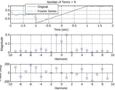
There are a number of different ways of graphically presenting the information in the Fourier series representation of a periodic function. The most common methods of presenting this information are by plotting the spectrum of the signal, or the power spectrum of the signal. In the following examples we will use the function

0 2

( ) 1 1

1 1 2

t

f t t t

t

1

− ≤ < − ⎧

⎪

=_⎨ − ≤ < ⎪ _{≤ <} ⎩

Spectrum of a Periodic Signal The spectrum of a periodic signal is a plot of the magnitude |c_k| against the corresponding frequencykω_o, and the phase against the corresponding frequency. Since our signal is periodic we only have values at

discrete frequencies (

k c

(

o

kω ), we do not know what happens in between these discrete frequencies so we do not “connect the dots”. Since ω_ois common to all of the discrete frequencies, we often plot against the harmonic k, rather than the frequency kω_o. Figure 2 shows the spectrum of f t( ).

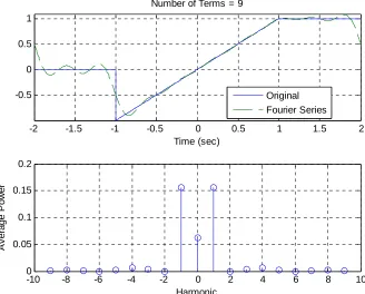
Power Spectrum of a Periodic Signal The power spectrum of a signal tells us how the power in the signal is distributed in frequency. To plot the power spectrum of a signal, we consider each term of the complex Fourier series, jk ot

k

c e ω . The average

power in this term is . The power spectrum indicates the power associated with

each frequency, and is thus a plot of against frequency

2

|c_k |

2

|c_k | kω_o or just the harmonic k.

In this plot we need to include both positive and negative frequencies. Figure 3 shows the power spectrum of f t( ).

Single-Sided Power Spectrum of a Periodic Signal Because the magnitudes of the coefficients are even (| | ), the powers associated with negative frequencies are the same as those associated with positive frequencies. Since only positive frequencies are realizable, we often just want to plot the power against positive frequencies. This gives us a single sided power spectrum, which is a plot of

versus the corresponding frequency |

k

c = c_−k|

2

0

2 2 2

0 1 2

|c | 2 |c | 2 |c | ... 2 |c_N |

0 0

0 ω 2ω ... Nω . Since the fundamental frequency ω₀is common to all of the frequency terms, we often just plot against the harmonics . Figure 4 shows the single sided power spectrum of

0 1 2 ... N

( )

f t .

power in decibels with respect to a one millivolt RMS reference. For the sinusoid at frequency kf₀, the average power in decibels is given by

10

10 log k

k dB

ref P P

P

= ,

where the power Pk represents the power spectrum coefficient

2

2c_k , and the power Pref

is the average power delivered to a one-ohm resistor by a one millivolt RMS sinusoid. We have

(

)

2

10 2

2

10 log dBmV

0.001

k k dBmV

c P

⎛ ⎞

⎜ ⎟

=

⎜ ⎟

⎝ ⎠

.

The units “dBmV” indicate that the reference for the decibels is a one millivolt RMSsinusoid.

-2 -1.5 -1 -0.5 0 0.5 1 1.5 2

-0.5 0 0.5 1

Time (sec) Number of Terms = 9 Original

Fourier Series

-10 -8 -6 -4 -2 0 2 4 6 8 10

0 0.2 0.4

Harmonic

M

a

gn

it

ud

e

-10 -8 -6 -4 -2 0 2 4 6 8 10

-200 0 200

Harmonic

P

has

e (d

eg)

Figure 2: The spectrum of f t( ).

-2 -1.5 -1 -0.5 0 0.5 1 1.5 2 -0.5

0 0.5 1

Time (sec) Number of Terms = 9

Original Fourier Series

-10 -8 -6 -4 -2 0 2 4 6 8 10

0 0.05 0.1 0.15 0.2

Harmonic

A

v

e

rag

e P

o

w

e

r

Figure 3: The power spectrum of f t( ).

-2 -1.5 -1 -0.5 0 0.5 1 1.5 2

-0.5 0 0.5 1

Time (sec) Number of Terms = 9

Original Fourier Series

0 1 2 3 4 5 6 7 8 9

0 0.1 0.2 0.3 0.4

Harmonic

A

v

e

rag

e P

o

w

e

r