Learning Personalized Attribute Preference via Multi-Task AUC Optimization

(1)

The Thirty-Third AAAI Conference on Artificial Intelligence (AAAI-19)

Learning Personalized Attribute Preference via Multi-Task AUC Optimization

Zhiyong Yang,

1,2

_{Qianqian Xu,}

3

_{Xiaochun Cao,}

1,2

_{Qingming Huang}

3,4,5∗

1_{SKLOIS, Institute of Information Engineering, Chinese Academy of Sciences, Beijing, China}

2_{School of Cyber Security, University of Chinese Academy of Sciences, Beijing, China} 3_{Key Lab of Intell. Info. Process., Inst. of Comput. Tech., CAS, Beijing, China}

4_{University of Chinese Academy of Sciences, Beijing, China}

5_{Key Laboratory of Big Data Mining and Knowledge Management, CAS, Beijing, China}

{yangzhiyong, caoxiaochun}@iie.ac.cn, [email protected], [email protected]

Abstract

Traditionally, most of the existing attribute learning methods are trained based on the consensus of annotations aggregated from a limited number of annotators. However, the consensus might fail in settings, especially when a wide spectrum of an-notators with different interests and comprehension about the attribute words are involved. In this paper, we develop a novel multi-task method to understand and predict personalized at-tribute annotations. Regarding the atat-tribute preference learn-ing for each annotator as a specific task, we first propose a multi-level task parameter decomposition to capture the evo-lution from a highly popular opinion of the mass to highly personalized choices that are special for each person. Mean-while, for personalized learning methods, ranking prediction is much more important than accurate classification. This mo-tivates us to employ an Area Under ROC Curve (AUC) based loss function to improve our model. On top of the AUC-based loss, we propose an efficient method to evaluate the loss and gradients. Theoretically, we propose a novel closed-form so-lution for one of our non-convex subproblem, which leads to provable convergence behaviors. Furthermore, we also pro-vide a generalization bound to guarantee a reasonable perfor-mance. Finally, empirical analysis consistently speaks to the efficacy of our proposed method.

Introduction

Visual attributes are semantic cues describing visual prop-erties such as texture, color, mood, and etc. Typical in-stances arecomfortableorhigh heeledfor shoes, and smil-ingor cryingfor human faces. During the past decade, at-tribute learning has emerged as a powerful building block for a wide range of applications (Song, Tan, and Chen 2014; Su et al. 2017; Wang et al. 2017; Yang et al. 2018).

The status quo of the attribute learning methods are mostly based on the global labels aggregated from few an-notators (Farhadi et al. 2009; Sadovnik et al. 2013; Luo et al. 2018). Recently, the rise of online crowd-sourcing platforms (like Amazon Mechanical Turk) makes collecting attribute annotations from a broad variety of annotators possible (Ko-vashka and Grauman 2015), which offers us a chance to re-visit the attribute learning. For consensus attribute learning, the underlying assumption is that the user decisions perturb

∗

The corresponding author.

slightly at random around the common opinion. However, different annotators might very well have distinct compre-hension regarding the meaning of the attributes(typical ones like ”open”, ”fashionable”). This suggests that the gap be-tween the personalized decisions and the common opinions could not be simply interpreted as random noises. What’s worse, one might even come to find conflicting results from different users. In such a case, there is a need to learn the consensus effects as well as personalized effects simultane-ously, especially when personalized annotations are avail-able. There are two crucial issues that should be noticed in this problem.

The grouping effects, lying in between consensus and per-sonalized ones, also play an essential role in understand-ing the user-specific attribute annotations. As pointed out in the previous literature (Kovashka and Grauman 2015), when understanding semantic attributes, humans often form the ”school of thoughts” in terms of their cultural backgrounds and the way they interpret the semantic words. Though per-sonalized effect might lead to conflicting results from differ-ent schools or groups, the users within the same group might very likely provide similar decisions. Moreover, different groups of people may probably favor distinct visual cues, as there is significant diversity among user groups. In other words, each user group should be assigned with a distinct feature subset. Accordingly, visual features and users should be simultaneously grouped to guarantee better performance. Furthermore, seeing that we cannot obtain the user-feature groups in advance, this constraint should be implicitly and automatically reflected via the structure of model parame-ters.

Unlike the consensus-based attribute predictions, prefer-ence learning is more important than label prediction for per-sonalized attribute learning, be it recommendation and im-age searching. Under such circumstances, when the attribute words are used as keywords or tags, it should be guaranteed that the positive labeled instances are ranked higher than the negative ones. It is well-known that the Area Under the ROC curve (AUC) metric exactly meets this requirement (Yang et al. 2017), and thus a better objective for our task.

(2)

problems we tackle. Our main contributions are listed as fol-lows: a) In the multi-task model, we propose a three-level decomposition of the task parameters which includes a con-sensus factor, a user-feature co-clustering factor and a per-sonalized factor. b) The proximal gradient descent method is adopted to solve the model parameters. Regarding our con-tribution here, we derive a novel closed-form solution for the proximal operator of the group factor and provide an effi-cient AUC-based evaluation method. c) Systematic theoret-ical analyses are carried out on the convergence behaviors and generalization bounds of our proposed method, while empirical studies are carried out for a simulation dataset and two real-world attribute annotation datasets. Both theoretical and empirical results suggest the superiority of our proposed algorithm.The codes are now available1

Related Work

Attribute learning Attribute learning has long been play-ing a central role in many machine learnplay-ing and computer vision problems. Along this line of research, there are some previous studies that investigate the personalization of at-tribute learning. (Kovashka and Grauman 2013) learns user-specific attributes with an adaption process. More precisely, a general model is first trained based on a large pool of data. Then a small user-specific dataset is employed to adapt the trained model to user-specific predictors. (Ko-vashka and Grauman 2015) argues that one attribute might have different interpretations for different groups of per-sons. Correspondingly, a shade discovery method is pro-posed therein to leverage group-wise user-specific attributes. Both works adopt two-stage or multi-stage models and even extra dataset. For the group modeling , (Kovashka and Grau-man 2015) only focus on user-level grouping while ignores the grouping effect of the features. Furthermore, the merit of AUC is also neglected. In contrast, we propose a fully auto-matic AUC-based attribute preference learning model where the user-feature coclustering effect is considered.

Multi-task Learning Multi-task learning aims at improv-ing the generalization performance by sharimprov-ing information among multiple tasks. Many efforts have been made to im-prove multi-task learning (Chen, Zhou, and Ye 2011; Yu, Tresp, and Yu 2007; Han and Zhang 2016; Zhao et al. 2018; Massias et al. 2018), etc. Recently, there is also a wave to in-vestigate the clustering and grouping based multi-task learn-ing (Zhou, Chen, and Ye 2011; Kumar and Daum´e 2012; Xu et al. 2015). Among this works, (Xu et al. 2015) is the most relevant work compared with our work since we adopt the co-clustering regularization proposed therein. However, our work differs significantly in that 1) our model is spe-cially designed for the attribute preference learning problem; 2) we propose a novel hierarchical decomposition scheme for the model parameters and; 3) we propose a novel closed-form solution for the proximal mapping of the co-clustering penalty; 4) we focus on efficient AUC optimization instead of regression or classification.

1

joshuaas.github.io/publication.html

Model Formulation

In this section, we propose a novel AUC-based multi-task model. Specifically, we first introduce the notations used in this paper, followed by problem settings in our model and a multi-level parameter decomposition. After that, we systematically elaborate two building blocks of our model: the AUC-based loss and evaluation, and the regularization scheme.

Notations

h·,·i denotes the inner product for two matrices or two vectors. The singular values of a matrixAare denoted as

σ1(A),· · ·, σm(A)such thatσ1(A) ≥ σ2(A) ≥ · · ·,≥ σm(A) ≥ 0.Iis the identity matrix,I[A]is the indicator

function of the setA,1denotes the all-one vector or matrix.

U(a, b)denotes the uniform distribution andN(µ, σ2₎

de-notes the normal distribution.⊗denotes the Cartesian prod-uct.

Problem Settings

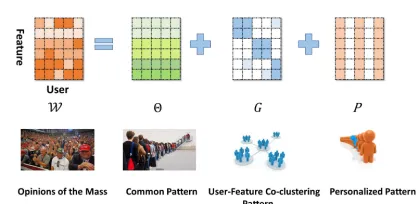
Figure 1: An illustration of the Multi-level Decomposition of the model parameters.

For a given attribute2_{, assume that we have}_U _{users who}

have annotated a given set of images. Further, we assume that the ith user labeled ni images with n+,i positive

la-bels andn−,inegative labels. S+,i = {k |y

(i)

k = 1}and

S−,i={k|y

(i)

k =−1}. We denote the training data as:S=

n

(X(1),y(1)₎_,_{· · ·}_,₍_X(U)

,y(U)₎o_{. For}_S_,_X(i)

∈ Rni×d

is the image feature inputs for the images that theith user labeled. Each row ofX(i)represents the extracted features for a corresponding image.y(i) _{∈ {−}₁_,₁_}ni _{is the}

corre-sponding label vector. Ify_k(i) = 1, then the user thinks that thekth image bears the given attribute, otherwise we have

y(_ki)=−1.

Taking advantage of the multi-task learning paradigm, the attribute preference learning for a user is regarded as a spe-cific task. Our goal is then to learn all the task modelsfi(x)

, where, for each task, a linear model is learned as the scor-ing function, i.ef(i)(x) =W(i)>x.

As shown in the introduction, it is natural to observe di-versity in personalized scores. However, this didi-versity could

2

(3)

by no means goes arbitrary large. In fact, we could inter-pret such limited diversity in a consensus-to-personalization manner. A common pattern is shared among the mass that captures the popular opinion. Different people might have different bias and preference, which drives them away from a consensus. Users sharing similar biases tend to form groups. The users within a group share similar biases to-wards the popular opinion based on a similar subset of the features of the object. Finally, a highly personalized user in a group tends to adopt an extra bias toward the group opinion. Mathematically, this interpretation induces a multi-level de-composition of the model weights :W(i)=θ+G(i)+P(i).

θ ∈ Rd×1 is the common factor that captures the

popu-lar global preference. G(i) ∈ Rd×1 is the grouping factor

for thei-th task. For mathematical convenience, we denote G = [G(1),· · ·,G(U)], and we haveG ∈ _Rd×U_._P(i) _is

the user-specific factor mentioned above. Similarly, we de-fineP = [P(1),· · ·,P(U)], andP ∈Rd×U. An illustration

of this decomposition is shown in Figure 1.

With all the above-mentioned settings, we adopt a general objective function in the form:

min θ,G,P

U

X

i=1

`i(f(i),y(i))+λ1R1(θ)+λ2R2(G)+λ3R3(P).

(1) Given (1), there are two crucial building blocks to be deter-mined:

• The empirical loss function for a specific useri:`i(·,·)

which directly induces AUC optimization;

• Regularization termsR1(θ),R2(G), andR3(P)which are defined by prior constraints onW.

In what follows, we will elaborate the formulation of two building blocks, respectively.

Regularization

For the common factorθ, we simply adopt the most widely-used`2 regularizationR1(θ) = kθk22to reduce the model

complexity. ForG, as mentioned in the previous parts, what we pursue here is a user-feature co-clustering effect. A pre-vious work in (Xu et al. 2015) shows that one way to si-multaneously cluster the rows and columns of a matrix in Rm×n into κ groups is to penalize the sum of squares of the bottom min{n, m} −κsingular values. This moti-vates us to adopt a regularizer onG in the following form :R2(G) = Pmin{d,U}

κ+1 σ

2

i(G).For any user i, a non-zero

columnP(i)is favorable only when she/he has a significant disagreement with the common-level and the group-level re-sults. This inspires us to defineR3(P) = kPk1,2norm to

induce column-wise sparsity.

Empirical Loss and Its Evaluation

Since the empirical loss is evaluated separately for each user, without loss of generality, the following discussion only fo-cus on a given useri.

Empirical Loss AUC is defined as the probability that a randomly sampled positive instance has a higher predicted score than a randomly sampled negative instance. Since we need to minimize our objective function, we focus on the loss version of AUC, i.e. the mis-ranking probability. Though the data distribution is unknown, given each user

ui andS+,i,S−,i defined in the problem setting, we could

attain an finite sample-based estimation of the loss version of AUC:

`(_{AU C}i) = X xp∈S+,i

X

xq∈S−,i

I(xp,xq)

n+,in−,i

,

where I(xp,xq) is a discrete mis-ranking

punish-ment in the form: I(xp,xq) = I[f(i)₍_x_p)_>f(i)₍_x_q)] + 1

2 I[f(i)₍_x

p)=f(i)(xq)].It is easy to see that` (i)

AU C is exactly

the mis-ranking frequency for user i on the given dataset. Unfortunately, optimizing this metric directly is an N P

hard problem. To address this issue, we adopt the squared surrogate losss(t) = (1−t)2 _{(Gao et al. 2016).}

Accord-ingly, the empirical loss`i(f(i),y(i))could be defined as:

`i(f(i),y(i)) = P

xp∈S+,i

P

xq∈S−,i

s

f(i)₍_x

p)−f(i)(xq)

n+,in−,i .

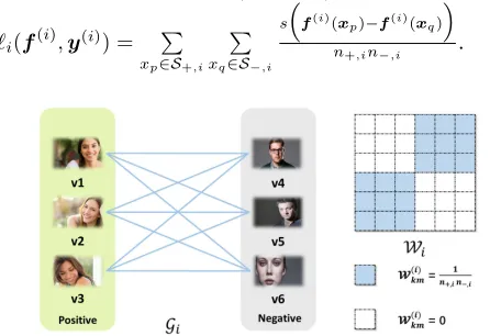
Figure 2: An illustration of the AUC graph, taking the anno-tation for attributesmileas an example.

Efficient AUC-based Evaluation At the first glance, the pair-wise AUC loss induces much heavier computation bur-dens than the instance-wise losses. It is interesting to note that, after carefully reformulating `i , the computational

burden coming from the pair-wise formulation could be perfectly eliminated. To see this, let us define a graph as

G(i) _{= (}_V(i)_,_E(i)_,_W(i)₎_{. The vertex set} _V(i) _{is the set}

of all the instances in (X(i),y(i)₎_{. There exists an edge}

(k, m) ∈ E(i) _{with weight}_W(i)

km =

1

n+,in−,i if and only

ify(_ki) 6=y(mi). This graph is further illustrated in Figure 2.

Given W(i)_{, the Laplacian matrix}_L(i)

of Gi could be

ex-pressed as: L(i) = diag(W(i)₁₎_{− W}(i)_. _{The empirical}

loss could be reformulated as a quadratic form defined by L(i): `i(f(i),y(i)) = 12(y˜

(i) ₋_f(i)₎>_L(i)₍_y_˜(i) ₋_f(i)₎_,

(4)

proposition gives a general result which suggests an efficient method to computeA>L(i)B, andA>L(i).

Proposition 1. For anyA∈Rni×a_and_B_∈

Rni×b_,where aandbare positive integers.A>L(i)B, andA>L(i)could be finished within O ni(a+b + ab)

= O(abni) and

O(ani), respectively.

Remark 1. According to this proposition, the complex-ity ofA>L(i)B could be reduced fromO(abn+,in−,i)to

O(ab(n+,i+n−,i)), whereas the complexity ofA>Lcould

be reduced fromO(an+,in−,i)toO(a(n+,i+n−,i)).

To end this section, we summarize our final objective function as:

(P∗) min θ,G,P

X

i

X

xp∈S+,i

X

xq∈S−,i

sW(i)>(xp−xq)

n+,in−,i

| {z }

L(W)

+λ1kθk22

| {z } R1(θ)

+λ2

min{d,U} X

κ+1

σ2_i(G)

| {z } R2(G)

+λ3kPk1,2

| {z } R3(P)

s.t W(i)=θ+G(i)+P(i)

For the sake of simplicity, we denote the empirical loss as

L(W), and we denote the objective function of (P∗) as

F(θ,G,P). Note thatL(W)should be a function ofθ,G, andP.

Optimization

We adopt the proximal gradient method as the optimizer for our problem. In this section, we introduce the outline of the optimization method and provide a novel closed-form solu-tion for the proximal operator ofR2(G).

For each iteration step k, giving a reference point Wrefk _{= (}_θrefk_,_Grefk_,_Prefk₎_{, then the proximal}

gradi-ent method updates the variables as :

θk :=argminθ 1 2 θ− ˜ θk 2 2+ λ1 ρk

kθk22 (2)

Gk:=argminG 1 2 G− ˜ Gk 2 F +λ2

ρk

min{d,U} X

κ+1

σ2_i(G)

(3)

Pk:=argminP 1 2 P − ˜ Pk 2 F + λ3 ρk

kPk1,2 (4)

where:θ˜k = θrefk ₋ 1 ρk

∇θL(Wrefk),G˜ k

= Grefk ₋

1

ρk

∇GL(Wrefk),P˜ k

=Prefk₋ 1 ρk

∇PL(Wrefk)

andρkis chosen with a line-search strategy, where we keep

on updatingρk =αρk, α >1until it satisfies:

L(W)<L(Wrefk_{) + Ψ}

ρk(Dθ) + Ψρk(DG) + Ψρk(DP).

(5)

Here Dθ = θ − θrefk_,_D_G ₌ _G ₋ _Grefk _and DP =P −Prefk_,_Ψ

ρk(DA) =

D

∇AL(Wrefk), DA

E

+ ρk

2 hDA, DAi.

Remark 2. The existence of suchρk is guaranteed by the

Lipschitz continuity of ∇L(W). Note that, we choose the last historical update of the parameter as the reference point i.e.Wrefk ₌_Wk−1_.

The solution to Eq.(2) and Eq.(4) directly follows the proximal operator of the `2 norm and the`1,2 norm (Sra,

Nowozin, and Wright 2012). For Eq.(3), we provide a novel closed-form solution in the following subsection.

A closed-form solution for G subproblem Note that Pmin{d,U}

κ+1 σi(G)2 is not convex, solving theG

subprob-lem is challenging. Conventionally, this probsubprob-lem is solved in an alternative manner (Xu et al. 2015) which is ineffi-cient and lack of theoretical guarantees. Thanks to the gen-eral singular value thresholding framework (Lu et al. 2015; Lin et al. 2017), we could obtain a closed-form optimal so-lution according to the following proposition.

Proposition 2. An Optimal Solution of (3) is:

G∗=UT_κ,λ₃ ρk

(Σ)V> (6)

whereUΣV> is a SVD decomposition ofG˜k,Tκ,cmaps

Σ = diag(σ1,· · ·,· · ·, σmin{d,U})to a diagonal matrix having the same size withTκ,c(Σ)ii= (₂_c1₊₁)I[i>κ]_σ

i.

Theoretical Analysis

Lipschitz Continuity of the Gradients of

L

(W

)

In the preceding section, we have pointed out that the Lip-schitz Continuity of the Gradients ofL(W)is a necessary condition for the success of the line search process to find

ρk. Now in the following theorem, we formally prove this

property as theoretical support for the optimization method. Theorem 1(Lipschitz Continuous Gradient). Suppose that the data is bounded in the sense that:

∀i, kX(i)k2=σXi <∞, n+,i≥1, n−,i≥1.

Given two arbitrary distinct parametersW,W0, we have:

k∇L(vec(W))− ∇L(vec(W0))k ≤γ∆W

where:γ= 3Up(2U+ 1) maxi

_n

iσX2i

n+,in−,i

,vec(W) =

[θ, vec(G), vec(P)],∆W =kvec(W)−vec(W0)k.

Convergence Analysis

Since the regularization term Pmin{d,U}

i=κ+1 σ 2

i(G) is

non-convex, the traditional sub-differential is not fully avail-able anymore. In this paper, we adopt the generalized sub-differential defined in (Rockafellar and Wets 2009; Liu et al. 2018). To guarantee a nonempty sub-differential set, the objective function must be lower semi-continuous. In our problem, it is obvious thatL(W),R1(θ),R2(P)are lower semi-continuous functions by their continuity. For the non-convex termPmin{d,U}

i=κ+1 σ 2

i(G), the following lemma shows

(5)

Lemma 1. The function Pmin{d,U}

i=κ+1 σ 2

i(G)is continuous

with respect toG.

Then the convergence properties of the proposed method could be summarized in the following theo-rem. Here we define ∆(θk) = θk+1−θk, ∆(Gk) =

Gk+1−Gk,∆(Pk) =Pk+1−Pk.

Theorem 2. Assume that the initial solutionsθ0,G0,P0 are bounded, with the line-search strategy defined in (5), the following properties hold :

• 1) The sequence {F(θk,Gk,Pk)}is non-increasing in the sense that :∀k,∃Ck+1>0,

F(θk+1,Gk+1,Pk+1)≤ F(θk,Gk,Pk)−

Ck+1(k∆(θk)k22+k∆(G

k )k2

F +k∆(P k

)k2

F)

(7)

• 2)limk→∞θk−θk+1= 0, limk→∞Gk−Gk+1= 0,

limk→∞Pk−Pk+1= 0.

• 3) The parameter sequences{θk}k,{Gk}k,{Pk}k are

bounded

• 4) Every limit point of{θk,Gk,Pk}k is a critical point

of the problem.

• 5)∀T ≥1,∃CT >0:

min

0≤k<T

k∆(θk)k22

≤CT

T , 0≤mink<T

k∆(Gk)k2F

≤CT T ,

min

0≤k<T

k∆(Pk)k2

F

≤ CT T .

Generalization Bound

Define the parameter setΘas :

Θ =

(θ,G,P) :pR1(θ)≤ψ1,R2(G)≤ψ2, kGk2≤σmax<∞,R3(P)≤ψ3

We have the following uniform bound.

Theorem 3. Assume that ∃∆χ > 0, all the instances are sampled such that, kxk ≤ ∆χ .Define C = (ψ1 +

p

ψ2+κ·σ2max+ψ3)ζ as ζ = ∆χC, we have, for all δ∈(0,1), for all(θ,G,P)∈Θ:

ED( X

i

`(_{AU C}i) )≤L(W) + U

X

i=1

B1

p

(niχi(1−χi))

+B2

s

ln(2

δ)

PU

i=1niχi(1−χi)

holds with probability at least 1 − δ, where B1 =

8√2C∆χ(1 +ζ),B2= 10 √

2(1 +ζ)ζ,χi=n_n+,i

i . The

dis-tributionD =⊗U

i=1(D+,i⊗ D−,i), where for useri,D+,i,

D−,iare conditional distributions for positive and negative

instances, respectively.

Remark 3. According to Theorem 2, the loss func-tion is non-increasing. For the solufunc-tion of our method

(θ∗,G∗,P∗), we then have:pR1(θ∗) ≤

q

F(θ0_,_G0_,_P0₎

λ1 ,

R2(G∗) ≤

F(θ0_,_G0_,_P0₎

λ2 ,R3(P∗) ≤

F(θ0_,_G0_,_P0₎

λ3 .

Mean-while, it could be derived from Theorem 2 that G∗

is bounded. By choosing ψ1 =

q

F(θ0_,_G0_,_P0₎

λ1 , ψ2 =

F(θ0_,_G0_,_P0₎

λ2 , ψ3 =

F(θ0_,_G0_,_P0₎

λ3 , all solutions chosen by

our algorithm belongs toΘ. Then, with high probability, all these solutions could reach a reasonable generation gap be-tween the expected 0-1 AUC loss metricED(Pi`

(i)

AU C)and

the estimated surrogate loss on the training dataL(W), with an orderO(PU

i=1 1 √

(niχi(1−χi))

).

Empirical Study

Experiment Settings

For all the experiments, hyper-parameters are tuned based on the training and validation set(account for 85% of the total instances), and the result on the test set are recorded.

Competitors

In this paper, we compare our model with the follow-ing competitors: Robust Multi-Task Learning (RMTL) (Chen, Zhou, and Ye 2011): RMTL aims at identifying irrel-evant tasks when learning from multiple tasks. To this end, the model parameter is decomposed into a low-rank struc-ture and group sparse strucstruc-ture. Robust Multi-Task Fea-ture Learning (rMTFL)(Yu, Tresp, and Yu 2007): rMTFL assumes that the model W can be decomposed into two com-ponents: a shared feature structure P(`1,2 norm penalty)

and a group-sparse structure Q (`1,2 norm penalty on its

transpose) that detects outliers. Lasso: The the `1-norm

regularized multi-task least squares method.Joint Feature Learning (JFL)(Nie et al. 2010): In JFL all the models are expected to share a common set of features. To this end, the group sparsity constraint is imposed on the mod-els via the`1,2norm.The Clustered Multi-Task Learning

Method (CMTL): (Zhou, Chen, and Ye 2011): CMTL as-sumes that the tasks could be clustered intokgroups. Then a k-means based regularizer is adopted to leverage such a structure. The task-feature coclusters based multi-task method (COMT)(Xu et al. 2015): COMT assumes that the task-specific components bear a feature-task coclustering structure.Reduced Rank Multi-Stage multi-task learning (RAMU) (Han and Zhang 2016): RAMU adopts a capped trace norm regularizer to minimize only the singular values smaller than an adaptively tuned threshold.

Note that since (Kovashka and Grauman 2013) adopts an extra data pool and (Kovashka and Grauman 2015) in-cludes extra initialization algorithms based on (Kovashka and Grauman 2013), our method is not compared with them for the sake of fairness.

Simulated Dataset

(6)

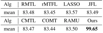
Table 1: AUC Comparison on Simulation Dataset

Alg RMTL rMTFL LASSO JFL

mean 83.48 83.45 83.57 83.49

Alg CMTL COMT RAMU Ours

mean 83.47 83.44 83.50 99.65

Table 2: Running Time Comparison (seconds): Original stands for the original AUC evaluation, wheres ours stands for our acceleration scheme.

ratio 20% 40% 60% 80% 100%

Orginal 18.57 74.22 151.86 268.55 nan Ours 3.06 5.50 8.65 12.46 15.82

of500,000 overall annotations. To capture the global infor-mation, we set θ as θ ∼ U(0,5) +N(0,0.52₎_{. In terms}

of the co-cluster nature, Gis produced with a block-wise grouping structure for feature-user co-cluster. Specifically, we create 5 blocks forG, namely:G(1 : 20,1 : 20),G(21 : 40,21 : 40), G(41 : 50,41 : 60), G(51 : 70,61 : 80)

andG(71 : 80,81 : 100). For each of the block, the ele-ments are generated from the distributionN(Ci,2.52)

(gen-erated via element-wise sampling) whereCi ∼ U(0,10)is

the centroid for the corresponding cluster and thus is shared among a specific cluster. For the elements that do not be-long to the 5 chosen blocks are set as 0. ForP ∈Rd×U, we

setP(:,1 : 5),P(:,10 : 15),P(:,20 : 25)randomly with the distributionU(0,10), while the remaining entries are set as 0. For each user, the scoring function are generated as s(i)₌_X(i)₍_θ₊_G(i)₊_P(i)_{) +}(i)_{, where}(i)_∈

R5000×1,

and(i) _{∼ N}₍₀_,₀_.₀₁2_I

5000). To generate the labels Y(i)

for eachi, the top 100 instances with highest scores are la-beled as 1, while the remaining instances are lala-beled as -1.

The performance of all the involved algorithms on the simulated dataset is recorded in Table 1. The correspond-ing results show that our proposed algorithm consistently outperforms other competitors. Specifically, our algorithm reaches an AUC score of 99.65, where the second best algo-rithm only attain a score of 83.57.

Besides the generalized performance, we could also ver-ify empirically the ability of our algorithm to recover the ex-pected structures on the parametersW. With the same sim-ulated dataset, we compare the parameterW learned from our proposed and the Ground Truth parameters in Figure 3. The results show that our proposed methods could roughly recover the expected group-based structure.

In Theorem 2, we have proved the convergence behav-ior of the proposed algorithm. To verify theoretical findings, we plot the loss and parameter evolution against the num-ber of iteration in Figure 4. In Figure 4-(a), we see that the loss function constantly decreases as the iteration proceeds, whereas in Figure 4-(b), it is easy to find that the parame-ter differencelog(kWt+1−Wtk)also keeps decreasing. All these empirical observations coincide with our

theoreti-(a) Ground-Truth (b) Learned Parameter

Figure 3: The Potential of our proposed method to Recover the Expected Structure of the Parameters

(a) Loss Convergence (b) Paramter Convergence

Figure 4: The Convergence Behavior On Simulation Dataset: a)shows the loss convergence, whereas b) exhibits the convergence property in terms of the parameters.

cal results.

To verify the efficiency of the proposed AUC evaluation scheme, we evaluate the running time of our algorithm with and without the AUC evaluation scheme. The resulting com-parison is recorded in Table 2 when different ratios of the dataset are adopted as the training set. As what exhibited here, the original algorithm without the efficient AUC eval-uation scheme gets slowly sharply when the training sample increases. When 100% samples are included in the training set, our server couldn’t finish the program within 1h due to the memory limit (24GB). We denote as nan correspond-ingly. In contrast, we can see an up to 20 times speed-up with the help of the proposed scheme in proposition 1.

Shoes Dataset

(7)

Table 3: Performance Comparison based on the AUC metric

Alg

Attibutes

Shoes Sun

BR CM FA FM OP ON PT CL MO OP RU SO

RMTL 79.31 84.99 66.90 85.08 75.67 67.22 75.14 69.36 62.71 75.28 67.91 69.23 rMTFL 70.90 83.78 67.27 85.91 73.71 65.21 77.11 69.27 62.15 75.80 68.16 68.76 LASSO 68.46 80.48 65.90 84.01 71.47 64.60 75.08 67.64 61.83 75.39 68.57 69.13 JFL 72.00 83.10 67.26 85.93 73.02 65.39 77.09 68.63 61.94 75.00 67.17 68.78 CMTL 74.54 85.16 68.21 85.32 75.06 68.17 77.62 72.55 66.61 79.78 72.34 72.82 COMT 84.24 88.68 69.66 89.19 80.93 72.99 80.62 70.69 63.72 76.93 69.43 70.44 RAMU 78.33 84.58 65.78 84.68 75.25 66.72 73.50 72.95 69.25 79.81 74.39 72.50 Ours 92.95 90.92 73.24 92.65 87.95 81.07 86.22 79.31 78.19 86.50 81.88 78.98

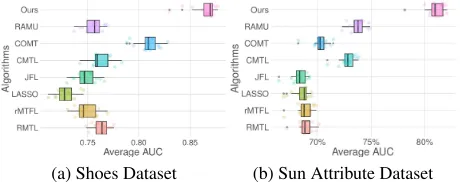
(a) Shoes Dataset (b) Sun Attribute Dataset

Figure 5: Average performances on all attributes of shoes dataset

labels. To this end, we remove the users who give less than 8 annotations for at least one of the classes.

The left half of Table 3 shows the average performance of the 15 repetitions with the experimental setting (BR: Brown, CM:Comfortable, FA:Fashionable, FM:Formal, OP: Open, ON: Ornate, PT:Pointy). Furthermore, in Figure 5 ,we visu-alize the average result over the 7 attributes for 15 repetitions with a boxplot. Accordingly, we could reach the conclusion that our proposed algorithm consistently outperforms all the benchmark algorithms by a significant margin.

Sun Attribute Dataset

The SUN Attributes Dataset (Patterson and Hays 2012), is a well-known large-scale scene attribute dataset with roughly 1,4000 images and a taxonomy of 102 discriminative at-tributes. Recently, in (Kovashka and Grauman 2015), the personalized annotations over five attributes are collected with hundreds of annotators. For each person, 50 images are labeled based on their own comprehension and prefer-ence. Overall, this dataset contains 64,900 annotations col-lected from different users. As for dataset preprocessing, we adopt almost the same procedure as the shoes dataset. The difference here is that we use the second last fc layer of the Inception-V3 (Szegedy et al. 2016) network as the input fea-ture. Furthermore, the PCA is done for each attribute pre-serving 90% of the total data variance.

The right half of Table 3 shows the average performance over 15 repetitions (CL:Cluttered, MO: Modern, OP:

Open-ing Area, RU: Rustic, SO: Soothe) , and Figure 5-(b) shows the average AUC scores over 5 attributes for the 15 repeti-tions. Similar to the shoes dataset, we see that our proposed algorithm consistently outperforms all the benchmark algo-rithms.

Conclusion

In this paper, we propose a novel multi-task model for learn-ing user-specific attribute comprehension with a hierarchical decomposition to model the consensus-to-personalization evolution and an AUC-based loss function to learn the pref-erence. Furthermore, we propose an efficient AUC-based evaluation method to significantly reduce the computational complexity of computing the loss and the gradients. Both theoretical and empirical analysis demonstrates the effec-tiveness of our proposed method.

Acknowledgment

This work was supported by the National Key R&D Pro-gram of China (Grant No. 2016YFB0800603). The re-search of Zhiyong Yang and Qingming Huang was sup-ported in part by National Natural Science Foundation of China: 61332016, 61650202 and 61620106009, in part by Key Research Program of Frontier Sciences, CAS: QYZDJ-SSW-SYS013. The research of Qianqian Xu was supported in part by National Natural Science Founda-tion of China (No.61672514, 61390514, 61572042), Beijing Natural Science Foundation (4182079), Youth Innovation Promotion Association CAS, and CCF-Tencent Open Re-search Fund. The reRe-search of Xiaochun Cao was supported by National Natural Science Foundation of China (No. U1636214, 61733007, U1605252), Key Program of the Chi-nese Academy of Sciences (No. QYZDB-SSW-JSC003).

References

Chen, J.; Zhou, J.; and Ye, J. 2011. Integrating low-rank and group-sparse structures for robust multi-task learning. InKDD, 42–50.

(8)

Gao, W.; Wang, L.; Jin, R.; Zhu, S.; and Zhou, Z. 2016. One-pass AUC optimization.Artif. Intell.236:1–29. Han, L., and Zhang, Y. 2016. Multi-stage multi-task learning with reduced rank. InAAAI, 1638–1644.

Kovashka, A., and Grauman, K. 2013. Attribute adaptation for personalized image search. InCVPR, 3432–3439. Kovashka, A., and Grauman, K. 2015. Discovering attribute shades of meaning with the crowd. International Journal of Computer Vision114(1):56–73.

Kumar, A., and Daum´e, H. 2012. Learning task grouping and overlap in multi-task learning. InICML.

Lin, Y.; Yang, L.; Lin, Z.; Lin, T.; and Zha, H. 2017. Factor-ization for projective and metric reconstruction via truncated nuclear norm. InIJCNN, 470–477.

Liu, R.; Cheng, S.; Liu, X.; Ma, L.; Fan, X.; and Luo, Z. 2018. A bridging framework for model optimization and deep propagation. InNIPS.

Lu, C.; Zhu, C.; Xu, C.; Yan, S.; and Lin, Z. 2015. General-ized singular value thresholding. InAAAI, 1805–1811. Luo, C.; Li, Z.; Huang, K.; Feng, J.; and Wang, M. 2018. Zero-shot learning via attribute regression and class proto-type rectification.IEEE Trans. Image Processing27(2):637– 648.

Massias, M.; Fercoq, O.; Gramfort, A.; and Salmon, J. 2018. Generalized concomitant task lasso for sparse multi-modal regression. InAISTATS, 998–1007.

Nie, F.; Huang, H.; Cai, X.; and Ding, C. H. 2010. Efficient and robust feature selection via joint l2,1-norms minimiza-tion. InIn NIPS, 1813–1821.

Patterson, G., and Hays, J. 2012. Sun attribute database: Discovering, annotating, and recognizing scene attributes. In CVPR, 2751–2758. IEEE.

Rockafellar, R. T., and Wets, R. J.-B. 2009. Variational analysis, volume 317. Springer Science & Business Media. Sadovnik, A.; Gallagher, A. C.; Parikh, D.; and Chen, T. 2013. Spoken attributes: Mixing binary and relative at-tributes to say the right thing. InICCV, 2160–2167. Song, F.; Tan, X.; and Chen, S. 2014. Exploiting relationship between attributes for improved face verification.Computer Vision and Image Understanding122:143–154.

Sra, S.; Nowozin, S.; and Wright, S. J. 2012. Optimization for machine learning. Mit Press.

Su, C.; Zhang, S.; Yang, F.; Zhang, G.; Tian, Q.; Gao, W.; and Davis, L. S. 2017. Attributes driven tracklet-to-tracklet person re-identification using latent prototypes space map-ping. Pattern Recognition66:4–15.

Szegedy, C.; Vanhoucke, V.; Ioffe, S.; Shlens, J.; and Wojna, Z. 2016. Rethinking the inception architecture for computer vision. InCVPR, 2818–2826.

Wang, Y.; Kwok, J. T.; Yao, Q.; and Ni, L. M. 2017. Zero-shot learning with a partial set of observed attributes. In IJCNN, 3777–3784.

Xu, L.; Huang, A.; Chen, J.; and Chen, E. 2015. Exploiting task-feature co-clusters in multi-task learning. InAAAI.

Yang, Z.; Zhang, T.; Lu, J.; Zhang, D.; and Kalui, D. 2017. Optimizing area under the ROC curve via extreme learning machines. Knowl.-Based Syst.130:74–89.

Yang, Z.; Xu, Q.; Cao, X.; and Huang, Q. 2018. From com-mon to special: When multi-attribute learning meets person-alized opinions. InAAAI, 515–522.

Yu, S.; Tresp, V.; and Yu, K. 2007. Robust multi-task learn-ing witht-processes. InICML, 1103–1110.

Zhao, M.; An, B.; Yu, Y.; Liu, S.; and Pan, S. J. 2018. Data poisoning attacks on multi-task relationship learning. InAAAI.