Abstract—A rigorous model for automatic modulation classification (AMC) in cognitive radio (CR) systems is proposed in this paper. This is achieved by exploiting the Kalman filter (KF) integrated with an adaptive interacting multiple model (IMM) for resilient estimation of the channel state information (CSI). A novel approach is proposed, in adding up the square-root singular values (SRSV) of the decomposed channel using the singular value decompositions (SVD) algorithm. This new scheme, termed Frobenius eigenmode transmission (FET), is chiefly intended to maintain the total power of all individual effective eigenmodes, as opposed to keeping only the dominant one. The analysis is applied over multiple-input multiple-output (MIMO) antennas in combination with a Rayleigh fading channel using a quasi likelihood ratio test (QLRT) algorithm for AMC. The expectation-maximization (EM) is employed for recursive computation of the underlying estimation and classification algorithms. Novel simulations demonstrate the advantages of the combined IMM-KF structure when compared to the perfectly known channel and maximum likelihood estimate (MLE), in terms of achieving the targeted optimal performance with the desirable benefit of less computational complexity loads.
Index Terms—Automatic modulation classification, Kalman filter, interacting multiple model, channel estimation.
I. INTRODUCTION
HEdesire to embed intelligent features, such as cognitive radio (CR), in emerging communication systems has recently received much attention. This is mainly attributed to the mechanisms that CRs possess to adapt to their changing surrounds [1]. The prime intention of CRs is to promote the awareness of efficient and sustainable spectrum utilization [17]. Unlicensed secondary users (SUs) featuring the intelligent strategies of CR systems are able to opportunistically share the unoccupied spectrum bands with licensed primary users (PUs) in order to achieve better spectral efficiency. This, of course, should occur without harming the
Manuscript received XX XX, 2018; revised XX XX 2018, and accepted XX XX, 2018. First published XX XX, 2018; current version published XX XX, 2018. The associate editor coordinating the review of this paper and approving it for publication was Dr. XXXX XXXX.
Ahmed O. Abdul Salam and Yim-Fun Hu are with the Faculty of Engineering and Informatics, University of Bradford, Bradford, BD7 1DP, UK (e-mail: [email protected], [email protected]).
Ray E. Sheriff is with the School of Engineering, University of Bolton, Bolton, BL3 5AB, UK (e-mail: [email protected]).
Saleh R. Al-Araji was formerly, and Kahtan Mezher is, with the College of Engineering, Khalifa University, P.O. Box 127788, Abu Dhabi, UAE (e-mail: [email protected], [email protected]).
Copyright (c) 2019 IEEE. Personal use of this material is permitted. However, permission to use this material for any other purposes must be obtained from the IEEE by sending a request to [email protected].
activities of PUs, and SUs should vacate particular spectrum bands upon PUs’ request without any untoward delay or disturbance. Specifically, CR systems not only need to perform spectrum sensing (SS) in the interested frequency bands but also need to interrogate the sensed signals to obtain additional information, such as the modulation scheme, in order to design improved dynamic spectrum access (DSA) strategies [18, 19].
As an intermediate stage between signal detection and demodulation, automatic modulation classification (AMC), sometimes referred to as automatic modulation recognition (AMR), plays a significant role in such adaptive aspects, whether of civilian or military nature. AMC mainly aspires to identify the modulation type of a noisy signal from a possible set of known patterns [2, 3]. Such a task should be flawlessly achieved irrespective of transmission constraints, such as large variations of signal-to-noise ratio (SNR) and severe fading. The consistency between AMC and DSA, in addition to adaptive coded modulation (ACM) techniques in general wireless communication systems, and particularly in CRs, is regularly reasserted. This is happening while most developers and operators are investigating emerging mobility scenarios, such as fifth-generation (5G) applications and spectrum opportunities under inconsistent channels [1, 17-19].
Two main categories of AMC techniques are prominent in survey literature [4, 5]: likelihood-based (LB); and feature-based (FB). The LB is considered optimal in the Bayesian sense if the channel state information (CSI) is known to the receiver, and also to the transmitter in the case of cooperative environment. The FB is built on a specific signal feature and is alleged to be less costly. In either method, if the work environment lacks coordination between the transmitter and the receiver, which is the case considered in this paper, then the whole process is conducted blindly. Generally, blind AMC systems are chiefly concerned with the automatic recognition of the modulation scheme of the received signals with limited or no prior knowledge, and hence are foreseen to radically improve the performance of the CR systems.
A number of recent studies in the context of LB and FB categories can be identified in the literature and a few samples of studies are considered here [20-26]. An LB algorithm for automatically identifying different quadrature amplitude modulation (QAM) and phase-shift keying (PSK) modulation schemes was given in [20]. The proposed algorithm maximizes a log-likelihood function (LLF) based on the known probability distribution associated with the phase or amplitude of the received signals for the most suitable modulation candidates. Their approach is blind as it does not
Automatic Modulation Classification Using Interacting
Multiple Model - Kalman Filter for Channel Estimation
Ahmed O. Abdul Salam,
Senior Member
,
IEEE
, Ray E. Sheriff, Yim-Fun Hu,
Senior Member
,
IEEE
,
Saleh R. Al-Araji,
Senior Member
,
IEEE
, Kahtan Mezher,
Senior Member
,
IEEE
need prior knowledge of the carrier frequency or the baud rate. An LB algorithm was also used in the AMC system for constellation identification of orthogonal frequency division multiplexing (OFDM) signal with index modulation, as an indicator of active subcarriers, in [21]. Two scenarios were proposed, known CSI and unknown CSI, with the latter conducted blindly by default. A rather different hybrid AMC approach that constitutes a combination of both the LB and FB schemes was proposed in [22], motivated by the claimed fact that the moments of the received signal are easy to compute and can provide a simple way for signal detection. The FB scheme in [22] was based on the high-order moments (HOMs) and high-order cumulants (HOCs). A useful complexity analysis and simulation comparisons with other state-of-the-art machine learning classifiers, such as genetic-programing based K-nearest neighbor (GP-KNN), linear support vector machine (LSVM) and Kolmogorov-Smirnov (KS) were provided [22].
Some notable studies on FB are selected for discussion [23-26] in the following, but several others also exist. The graph, constructed from the Fourier transform of the second and fourth powers of the received signal, as a discrimination feature was exploited for classification in [23]. This FB classifier was claimed to have no dependence on the CSI or SNR estimation, nor did it need timing or frequency offset corrections. An end-to-end convolution neural network (CNN) based AMC (CNN-AMC), which automatically extracts features from the long symbol-rate observation sequence along with the estimated SNR was proposed in [24]. Such a classifier was thought of as a competent track to the FB, and the complexity of which alongside the conventional LB was presented. Another blind AMC method, based on the combination of elementary and cyclic cumulants, was proposed in [25]. The elementary cumulant was used to decide whether the constellations are from real, circular, or rectangular class, which was referred to as macro classifier. While, on the other hand, the cyclic cumulant was used to classify modulation within a subclass, which was referred to as micro classifier. A modulation-constrained clustering with unknown channel matrix and noise variance for multiple-input multiple-output (MIMO) systems was addressed in [26]. The AMC task was altered into a number of clustering problems, by projecting the sliced received signals into clusters, one for each modulation pattern. The final outcome was then decided by using the ML criterion applied to each intrinsic cluster.
Concluding from the above, the demand for accurate channel modelling and estimation has been noticeably emphasized. The finite state Markov chain (FSMC) has recently gained much attention in the modelling of wireless channels [1, 6, 7, 11]. Such channels are broadly categorized as a type of jump Markov linear systems (JMLSs), whose parameters evolve according to the realization of an FSMC model. A recent study, considering an LB classifier and featuring the Baum-Welch (BW) procedure for forward-backward computation of fading variable using the hidden Markov model (HMM) can be identified in [27]. From another perspective, the interacting multiple model (IMM) has been
commonly adopted to cope with the dynamic changes of various aerospace, navigation and signal processing systems [6, 7]. The IMM algorithm is widely involved in determining various processes, the underlying parameters of which evolve in the premises of FSMC and HMM approximations.
The Kalman filter (KF), on the other hand, is generally considered as one of the best optimum estimation algorithms that can be applied to a variety of vibrant systems [6, 10]. In this paper, we propose to employ the robust IMM geared to a bank of KFs for the purpose of CSI estimate adaptation and, thereby, render the AMC performance more efficient in CR systems. That is in the sense that several individual KFs can be constructed to mimic different fading effects, which are anticipated to evolve similarly to the FSMC or the HMM processes. The IMM algorithm then statistically combines the KFs’ outputs as per the weighing factor assigned to each KF branch based on how accurately each copes with the presumed dynamic range of fading variants.
To the best of our knowledge, this paper, for the first time, proposes integrating IMM with the KF structures to adaptively track and follow the CSI and fading attributes. Amending the combined IMM-KF structure for adaptive CSI estimation and aiming at the consolidation of AMC systems is proposed in this paper, which has not been addressed elsewhere in the literature. Simulations are conducted with reference to the classical maximal likelihood (ML) channel estimators [2, 3]. The results validate the performance and efficiency of the integrated IMM-KF structure in the AMC paradigm.
A. Contributions
The demand for reliable AMC strategies in the design of CR systems has become increasingly pressing with the advent of new communication technologies. With this in mind, this paper aims to design a consistent and seamless AMC model with acceptable computational budget. The most notable contributions are as follows:
Employing the SVD, equipped with the MRC, to perform the MIMO eigenchannel decomposition for space reduction and to render tractable CSI estimation.
Developing a new approach of adding up the effective eigenemode transmission parameters instead of relying on individual ones and hence maintaining the power of all.
Featuring a novel AMC approach based on the combined IMM-KF structure for resilient CSI estimation to enhance the LB classifier performance.
Applying the IMM-KF output to the EM algorithm and performing the iterative computation of overlapped cycles concerned with the CSI estimation and signal detection.
Assessing the underlying complexity and computational requirements of the AMC based on IMM-KF, which advantageously reveals that it has less overheads compared to the classical ML for CSI estimation.
B. Mathematical Notations
lowercase letters denote vectors; and non-boldface lowercase letters denote scalar variables. The operators (. )∗, (. )T, (. )†
and ‖. ‖2 denote conjugate, transpose, Hermitian (conjugate transpose) and Frobenius norm, respectively. The operator ∀
means for all elements that belong to, or ∈, a certain space. The minimization is 𝑚𝑖𝑛(. ), maximization is 𝑚𝑎𝑥(. ), the summation is 𝑠𝑢𝑚(. ), while 𝑑𝑖𝑎𝑔[. , . , . ] represents the diagonal entries of a matrix. 𝔼(. ) is the statistical expectation,
Pr(. ) is the probability, ln(. ) is the natural logarithmic, and
e𝑥𝑝(. ) is the exponential function.
C. Outline
The remainder of this paper is organized as follows. Section II introduces the system modelling; Section III presents the space reduction techniques; Section IV discusses the basics of modulation classifications; Section V discusses the channel modeling and KF estimation; Section VI addresses the FSMC channel modeling and IMM adaptation, Section VII presents the joint channel estimation and data detection; Section VIII is concerned with the expectation-maximization; Section IX elaborates on the complexity analysis, and Section X is devoted to the numerical results and is followed by the concluding remarks.
II. SYSTEM MODELING
Consider a linearly modulated signal transmitted through a time-variant fading channel of Rayleigh characteristics using a
𝑁𝑡× 𝑁𝑟MIMO system. The received baseband signal in this case is denoted by [2-5]
𝑦𝑖(𝑘) = ∑[ℎ𝑖,𝑗(𝑘)𝑥𝑗,𝑚(𝑘) + 𝑛𝑖(𝑘)],∀𝑘 ∈ 𝐾
𝑁𝑡
𝑗=1
(1)
where 𝑦𝑖(𝑘) is the 𝐾-length complex-valued sequence received on antenna 𝑖, ℎ𝑖,𝑗 is the channel parameters, 𝑥𝑗,𝑚(𝑘) is the transmitted signal on antenna 𝑗 and associated with the constellation set mapping,𝒞𝑚as the𝑚th modulation and m = 1,…M, which can be of any priori known type, and 𝑛𝑖(𝑘) is the additive white Gaussian noise (AWGN) of zero mean and variance 𝜎𝑛2𝑖. The symbols {𝑥𝑗,𝑚(𝑘)}𝑚=1
𝑀
are assumed uniform and independent over 𝒞𝑚 space with zero mean and variance one. Revising (1) in matrix form yields
𝒀(𝑘) = 𝑯(𝑘)𝑿(𝑘) + 𝑵(𝑘),∀𝑘 ∈ 𝐾 (2)
where 𝑯 is the 𝑁𝑡× 𝑁𝑟 channel matrix and the coefficients of which are assumed to be statistically independent Gaussian distributed complex circular random variables of zero mean and unknown variance, which is to be estimated. The AWGN vector𝑵 is given by 𝒞𝒩~(0, 𝜎𝑛2𝑰) and 𝑰 is an identity matrix.
III. SPACE REDUCTION
Modeling simplification using space reduction techniques is highly desirable, especially for online streaming applications such as the AMC systems. Aiming at an effective and straightforward CSI estimate, two powerful yet essentially equivalent simplification strategies can be applied. The first
strategy is called eigenmode transmission (ET), while the second is beamforming (BF); both are prevalent in the literature [8, 9]. While the singular value decomposition (SVD) can be applied to both strategies, BF is more related to maximum-ratio combining (MRC) at the transmitter, often called (MRT). Both strategies, however, separate the MIMO channel into 𝑅 = 𝑚𝑖𝑛{𝑁𝑡, 𝑁𝑟} virtually separated parallel channels [12-14] with a gain of 𝑔𝑟=√𝜆𝑟, which is the square root of the 𝑟th eigenvalue, 𝜆𝑟 of 𝑯𝑯† or 𝑯†𝑯.
The 𝑁𝑟× 𝑁𝑡 channel matrix 𝑯, with rank 𝑅 = 𝑚𝑖𝑛(𝑁𝑡, 𝑁𝑟) has an SVD representation given by 𝑯 = 𝑼𝜮𝑽†, where 𝑼 and
𝑽 are 𝑁𝑟× 𝑅 left and 𝑁𝑡× 𝑅 right matrices to satisfy 𝑼𝑼†=
𝑽𝑽†= 𝑰
𝑅, 𝜮 = 𝑑𝑖𝑎𝑔[σ1, σ2, … , σ𝑅] with σ𝑖≥ 0 and σ𝑖≥
σ𝑖+1, where σ𝑖 is the 𝑖th singular-value of the channel. The columns of 𝑽 and 𝑼 are also known as the left input and right output singular vectors, respectively. Now, 𝑯𝑯† is a 𝑁
𝑟× 𝑁𝑟 semi-definite Hermitian matrix. Let the eigen decomposition of 𝑯𝑯† be 𝑸𝝀𝑸† where 𝑸 is an 𝑁𝑟× 𝑁𝑟 matrix satisfying
𝑸†𝑸 = 𝑸𝑸†= 𝑰
𝑁𝑟 and 𝝀 = 𝑑𝑖𝑎𝑔[𝜆1, 𝜆2, … , 𝜆𝑅] with random variable eigenvalues 𝜆𝑖≥ 0, sorted in a descending order
𝜆𝑖≥ 𝜆𝑖+1 and have Chi-square distribution and 2𝑁𝑡𝑁𝑟 degrees of freedom [14]. Then, 𝜆𝑖= σ𝑖2 for 𝑖 ∈ {1, 2, … , 𝑅} and 𝜆𝑖= 0
for 𝑖 ∈ {𝑅 + 1, 𝑅 + 2, … , 𝑁𝑟}.
After applying any of the transmission strategies and with the support of spatial-temporal matched filtering (STMF) to maximize the energy of displaced signals, (1) and (2) can be reduced to the following expression of total received signal
𝑦(𝑘) = ∑[√𝜆𝑟𝑥𝑟,𝑚(𝑘) + 𝑛𝑟(𝑘)],∀𝑘 ∈ 𝐾, ∀𝑚 ∈ 𝑀
𝑅
𝑟=1
(3)
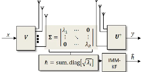
where the noise statistical characteristics remain intact after all mathematical manipulations and the received signal elements are hence decoupled and can be processed separately, since they are independent and identically distributed (iid) statistical processes. Further simplification can also be proposed here by having an effective channel parameter expressed by summing the diagonal entries ℏ = 𝑠𝑢𝑚. 𝑑𝑖𝑎𝑔[√𝜆𝑟], i.e., summing up the square-root of singular values (SRSV), to alter (3) as follows
𝑦(𝑘) = ℏ(𝑘)𝑥𝑚(𝑘) + 𝑛(𝑘),∀𝑘 ∈ 𝐾, ∀𝑚 ∈ 𝑀 (4)
in the adaptive transmission rates and channel capacities and full diversity can be also reached under certain conditions [12, 13]. As this paper is favorably inclined towards the ET strategy, a blind CSI estimation on the receiver side is considered without any back return to the transmitter. This is the normal situation in vast non-cooperative wireless communication systems; otherwise there will be no need for the AMC if both the transmitter and the receiver are originally cooperative.
Other interesting subspace reduction forms aligned with the task of signal identification can also be found in the literature. For example, the quadrature left decomposition (QLD) and the quadrature right decomposition (QRD) techniques were discussed in [15, 16]. Both studies suggested further space reduction by using the WRD, or WLD, approach, where W, R, and L stand for matrices’ names used in the analysis therein, which can be attended by swapping particular layers in the punctured structures. The complexity overheads were evaluated and major savings were claimed while achieving near optimum classification performances.
Inspired by the above, the substantiation of the new paradigm proposed in this paper becomes quite apparent. The proposed approach here departs from other roadmaps suggested elsewhere in the sense that it is not concerned with the factorization of the channel covariance matrix. The core idea of the proposed paradigm is mainly centered on the eigenvalues of the decomposed channel and, instead of being treated individually, they are summed to generate a new single parameter. This parameter symbolizes the variant effects of a block-fading channel that is readily available to streamline the IMM-KF estimation algorithm. Such an approach is believed to be unique, with no evidence that it has been experimented elsewhere previously.
The new concept of total effective SRSV, which is mathematically equivalent to the Frobenius norm, is dubbed Frobenius ET (FET) in this paper. The simplified diagram of the proposed eigen-based adaptive IMM-KF for CSI estimation is portrayed in Fig. 1 below.
Fig. 1. Simplified diagram of the proposed adaptive CSI estimator.
IV. MODULATION CLASSIFICATION
This section is centered on the LB analysis, which is intrinsic to the premise of Bayes system. The eventual ML classifier is realized by conducting a multiple hypothesis test (MHT), whereby ℋ𝑚 is arbitrarily assigned to the 𝑚th
modulation type out of 𝑀 potentials. The MHT is a composite methodical problem with strong links to the joint and conditional probability density functions (PDFs) of unknown parameters [2-5]. The PDF below is for the system in (4)
𝑝(𝒚|𝒙, 𝚯) = ∏ ∑ 1
𝑀 1
√2𝜋𝜎𝑛
𝑒𝑥𝑝 (−|𝑦𝑘− ℏ𝑘𝑥𝑚,𝑘|
2
2𝜎𝑛2
)
𝑀
𝑚=1 𝐾
𝑘=1
(5)
where 𝒚 is the vector for all received samples ∀𝑘 ∈ 𝐾,𝚯 =
[ℏ𝜎𝑛]𝑇 is the vector of unknown parameters and the time
index is changed for simplicity to down-script. Optimum or semi-optimum solutions to the composite MHT task can be attempted by appraising the unknown parameters as random variables (RVs). Four different ML application scenarios can consequently be distinguished, namely: the average likelihood ratio test (ALRT); generalized likelihood ratio test (GLRT); hybrid likelihood ratio test (HLRT); and quasi likelihood ratio test (QLRT) [2-5]. Probing into the ALRT reveals the likelihood of 𝒚 under ℋ𝑚 is attained by averaging the PDF over unknown signal constellations and nuisance parameters
ΛALRT𝑚 (𝒚) = 𝔼𝒙𝔼𝚯[𝑝(𝐲|𝒙, 𝚯)] (6)
where 𝔼𝑥[. ] and 𝔼𝚯[. ] are the expectations operators. The above ALRT algorithm assumes the statistical characteristics of unknown RVs are either exactly defined or fitted to the best, which is a vastly tedious task in reality. It is therefore practically not feasible in most CR applications, especially under large constellation size, due to its highly nonlinear complexity and computational burdens. The ALRT merely signifies the upper-bound (UB) limit for other algorithms.
From another perspective, the GLRT algorithm is taken as being equivalent to ALRT, providing that the ML estimate (MLE) of nuisance parameters is used and, therefore, the performance of which is unavoidably inferior. Applying the GLRT algorithm under nested constellations is also considered awkward [4]. While on the other hand, the averaging is conducted over the unknown symbols only in the HLRT and QLRT algorithms, and eventually the suitable estimate 𝚯̂
replaces 𝚯 as follows
Λ𝑚
(Q)HLRT
(𝒚) = 𝔼𝒙[𝑝(𝒚, 𝚯̂|𝒙)] (7)
The MLE for the sought parameters is at the heart of HLRT, while the QLRT may use other estimation tools. The non-data aided (NDA) provision suggests that both algorithms can be realized blindly or semi-blindly.
Recall that the natural logarithm is monotonically increasing and Λ𝑚 is positive-definite, the log-likelihood ratio (LLR) defined as ℒ𝑚= ℒ(𝒚/ℋ𝑚) = 𝑙𝑛(Λ𝑚) is proved useful to simplify the MC decision making. The decision criterion for binary HT (BHT) problem is hence constructed as the ratio between two observations ℋ𝑚 and ℋ𝑚′ with prior probabilities 𝑃𝑚 and 𝑃𝑚′, respectively, as given below
𝑙𝑛ℒ(𝐲/ℋ𝑚)
ℒ(𝐲/ℋ𝑚′)= ℒ𝑚− ℒ𝑚
′ 𝑙𝑛
𝑃𝑚
𝑃𝑚′ <ℋ
𝑚′
>ℋ𝑚 (8)
BHT can be uniformly generalized overall applicable 𝑀
hypotheses space to yield the following detection rule
𝒞̂𝑚= 𝑎𝑟𝑔𝑚∈{1,2,…,𝑀}𝑚𝑎𝑥(ℒ𝑚) (9)
The main task of MC is to maximize the LLR functions comprised in MHTs and decide the best modulation candidate with as fewer errors as possible. The classifier performance can be quantified in terms of the individual probability of correct classification 𝑃𝐶𝐶, which is the probability under hypothesis ℋ𝑚 given that modulation 𝑚 is the accurate modulation
𝑃𝐶𝐶= Pr(correct|ℋ𝑚) = Pr[ℒ𝑚> ℒ𝑚′],∀𝑚 ≠ 𝑚′ (10)
The overall average probability of correct classification is not a favorable performance indicator since the individual probabilities cannot be assessed separately [3].
V. CHANNEL MODELING AND KFESTIMATION
Efficient CSI estimation is crucial to the performance of higher-order modulations; KFs are very attractive in such domains [6, 10]. An accurate approximation for the channel modeling needs is to be investigated first before embarking on the development of KF algorithms. The following 1st-order autoregressive (Gauss-Markov) AR(1) model can embrace most of the channel dynamics and lead to effective tracking
ℏ(𝑘 + 1) = ℏ(𝑘) + 𝑤(𝑘) (11)
where 𝑤(. ) is the state AWGN denoted by 𝒞𝒩~(0, 𝜎𝑤2). The Jakes-Clarke (JC) channel model is commonly adopted as one of the best statistical models for inferring the random fading effects [6, 10, 11]. It can be easily approximated by using the AR(1) model as described in (11) above, and in this case ℏ
represents a zero-mean complex random process with autocorrelation function 𝔼{ℏ(𝑘)ℏ∗(𝑘 − 𝑚} = 𝜎
ℎ2𝐽0(2𝜋𝑓𝐷𝜏/
𝑓𝑠), where 𝐽0(. ) is the zero-order Bessel function, 𝑓𝐷 is the maximum Doppler frequency, 𝜏 is the time delay, and 𝑓𝑠 is the sampling frequency [6, 10, 11].
The channel state and observation models given in (11) and (4), respectively, are essential to construct the recursive scalar KF algorithms. The definitions of the following terms are due [7, 8]; ℏ̂𝑘|𝑘−1 and ℏ̂𝑘|𝑘 for the state prediction and estimate at step 𝑘, and 𝑃𝑘|𝑘−1≜ 𝔼 {(ℏ𝑘|𝑘− ℏ̂𝑘|𝑘−1)
2
} and 𝑃𝑘|𝑘≜
𝔼 {(ℏ𝑘|𝑘− ℏ̂𝑘|𝑘)
2
} for the prediction and estimation errors’ covariances, respectively. The predictions for the system model described in (11) can be obtained as below
{ ℏ̂𝑘|𝑘−1= ℏ̂𝑘−1|𝑘−1 𝑃𝑘|𝑘−1= 𝑃𝑘−1|𝑘−1+ 𝜎𝑤2
(12)
and the state estimate can be recursively updated as follows
{ ℏ
̂𝑘|𝑘 = ℏ̂𝑘|𝑘−1+ 𝐺𝑘𝑧𝑘
𝐺𝑘 ≜ 𝑃𝑘|𝑘−1𝑥̂𝑙,𝑘−1T 𝑆𝑘−1
𝑃𝑘|𝑘 = (1 − 𝐺𝑘)𝑃𝑘|𝑘−1
(13)
where 𝐺𝑘 is the KF gain at step 𝑘, the residual sequence
𝑧𝑘 = (𝑦𝑘− 𝑥̂𝑙,𝑘−1ℏ̂𝑘|𝑘−1) is of covariance
𝑆𝑘 = 𝑥̂𝑙,𝑘−1𝑃𝑘−1|𝑘−1𝑥̂𝑙,𝑘−1T + 𝜎𝑤2, and 𝑥̂𝑙,𝑘−1 is a priori classified symbol whereas superscript T denotes transpose.
VI. FSMC AND IMMADAPTATION
The information-theoretic approach of popular 1st-order FSMC is a good approximation of random channel variations and agrees with the JC model. A single transition probability in the FSMC model 𝜋ℏ1→ℏ2,𝑘 represents the prior probability of a channel transiting from state ℏ𝑖 to state ℏ𝑗 at a particular step 𝑘 as given below [1]
𝜋𝑘
𝑖,𝑗
= 𝜋ℏ𝑖→ℏ𝑗,𝑘 = Pr{ℏ𝑗,𝑘|ℏ𝑖,𝑘−1} (14)
The current channel is hence only associated with the previous state, and statistically independent of all past and future states, i.e.,𝜋𝑘𝑖,𝑗= 0 for |𝑖 − 𝑗| > 1. The transition probability 𝝅𝑘 matrix can be formed with entries as denoted in (14) for self and immediate neighboring cells accordingly.
Building on the above, a scalar KF can be arbitrated for a span of discrete channel states and hence facilitate the IMM algorithms appropriately. For a 𝒥-bank of KFs, these algorithms comprise the following core processing steps [7].
1) Interact: Action conditional and predicted probabilities
𝜇𝑘−1|𝑘−1𝑖|𝑗 =𝜋𝑘
𝑖,𝑗
𝜇𝑘−1|𝑘−1𝑖
𝜇𝑘|𝑘−1𝑗 ; 𝜇𝑘−1|𝑘−1
𝑖 = ∑ 𝜋
𝑘 𝑖,𝑗
𝜇𝑘−1|𝑘−1𝑗
𝒥
𝑗=1
(15)
And then mix the state estimates and covariance
ℏ
̅𝑘−1|𝑘−1𝑖 = ∑ 𝜇 𝑘−1|𝑘−1 𝑖|𝑗
ℏ ̂𝑘−1|𝑘−1𝑖 𝒥
𝑗=1
(16)
𝑃̅𝑘−1|𝑘−1𝑖 = ∑ 𝜇𝑘−1|𝑘−1 𝑖|𝑗
[𝑃𝑘−1|𝑘−1𝑗
𝒥
𝑗=1
+ (ℏ̅𝑘−1|𝑘−1𝑖 − ℏ̂𝑘−1|𝑘−1 𝑗
)2]
2) Filter: Individual KF performs its usual filtering tasks. 3) Update: Update each KF probability as per residual error
∆𝑘𝑖=
𝑒𝑥𝑝 (−(1/2)(𝑧𝑘𝑖)
2
(𝑆𝑘𝑖) −1
)
√|2𝜋𝑆𝑘𝑖| (17)
𝜇𝑘|𝑘𝑖 =
𝜇𝑘|𝑘−1𝑖 ∆ 𝑘 𝑖
∑𝒥𝑗=1𝜇𝑘|𝑘−1𝑗 ∆𝑘𝑗
4) Combine: Weight the state estimate and its covariance
ℏ
̂𝑘|𝑘 = ∑ 𝜇𝑘|𝑘𝑖 ℏ̂
𝑘|𝑘 𝑖 𝒥
𝑖=1 (18)
𝑃𝑘|𝑘= ∑ 𝜇𝑘|𝑘𝑖 [𝑃𝑘|𝑘𝑖 + (ℏ̂𝑘|𝑘− ℏ̂𝑘|𝑘𝑖 ) 2
]
𝒥
𝑖=1
This apparently turns out to be a typical integer least-squares (LS) or minimum variance (MV) detection problem.
VII. JOINT CHANNEL ESTIMATION AND DATA DETECTION
Capitalizing on the above, it has become apparent for the requirement to promote a joint link between the AMC and CSI estimation strategies. In the strict sense of an AMC framework, the awareness of such joint channel estimation and data detection, dubbed here (JCEDD), is well established. The unknown CSI parameters that are accurately and seamlessly estimated would decisively contribute towards the successful operation of the AMC systems. Given such estimations are mostly encountered in uncertain environments, the AMC empowered by CSI estimate should be sufficiently intelligent to operate under adverse and complex situations, while the structure needs to be less bulky in order to afford real-time processing as practically feasible. Therefore, this section aims to shed more light into the JCEDD approach along with supplementary options, which have been proved to be useful for the AMC and CSI estimation integrated performance. Research on the JCEDD approach in the framework of blind AMC applications is extensive, and only a few notable studies are mentioned herein [10, 28-34]. The interest in JCEDD techniques is not new and growth is expected to continue, not only with AMC applications, but also with other pinnacle functions of CR systems like the SS and ACM.
An overview of the JCEDD blind techniques can be obtained from [28]. Generally, blind techniques can be branched into two main streams, either deterministic or statistical, depending on how the input signal is modelled [28]. If the modelling assumes the input is a random variable with predefined statistics, the corresponding blind technique is to be statistical. On the other hand, if the modelling does not have any a priori description of the input random variable, or the statistics of which are available but are not exploited, and does not have a statistical description, the corresponding blind technique algorithm is called deterministic.
The JCEDD can be applied to any kind of unknown parameters of interest, which evolve around the core parameter represented by the alphabet symbols. Moreover, the JCEDD algorithm can be approached via iteratively exchanging information between the CSI estimator and the signal detector, noting that the detection and classification words can be used interchangeably in the literature and also in this work. The information exchange process is decomposed into two optimization loops, the outer and the inner. The outer loop is a global optimization algorithm, which searches for an optimal CSI estimate, while the inner loop is an ML algorithm that identifies the transmitted symbols [28-33]. These loops are interweaved, and sometimes called the upper level and the lower level, in tandem.
In [28], the repeated weighted boosting search algorithm was used for CSI estimate at the outer loop, which searches the MIMO channel space by evolving a population of MIMO channel matrices. While at the inner loop, the optimized hierarchy reduced search algorithm aided detector, which is an
advanced extension of the complex sphere decoder, was used [28]. The signal identification by classifying both the modulation type and the STBC scheme in MIMO systems was considered as a joint classification problem in [32]. The JCEDD was also extended to MIMO-OFDM systems in the framework of sparse Bayesian learning techniques in [10]. It was also applied to the unknown co-scheduled user’s modulation constellation size as part of the MU-MIMO detector in [33]. The per-survivor processing of best optimization path using the VA algorithm as an effective trellis search engine in the context of JCEDD was elaborated in [29, 30]. The KF algorithm for CSI estimation was employed in [10, 34], whereas the GA procedure was implemented in [30].
On the side of design tools necessary for the JCEDD algorithm, the first step usually begins by tailoring a minimization cost function, which should be suitably assigned to reflect on all the parameters of concern. Considering the MIMO configuration, this can be done by applying the MLE on the transmitted symbols 𝑿𝒊 and the channel matrix 𝑯 and then maximizing the joint conditional PDF over 𝑿 and 𝑯
together. Alternatively, this can be achieved by minimizing the following joint cost function [28-34]
ℱ(𝑿,̌ 𝑯̌ ) = ∑‖𝒀 − 𝑯𝑿‖2
𝐾
𝑘=1
(20)
where all the constants have been ignored as they will cancel each other while calculating LRTs. Namely, the joint ML for channel and data estimation is obtained as below [28-34]
(𝑿̂, 𝑯̂ ) = 𝑎𝑟𝑔{𝑚𝑖𝑛𝑿̌,𝑯̌[ℱ(𝑿,̌ 𝑯̌ )]} (21)
As can be seen from (21), the search for the optimal joint ML result is over the entire discrete space of all the possible transmitted alphabets and the MIMO channel matrix, which is computationally prohibitive in reality. Therefore, the complexity of such an optimization process needs to be reduced to tractable levels. This can be done if each single search cycle is decomposed into two iterative loops: firstly, over all the possible data symbols; and then over all the channel matrix entries. This can be formed as below [30, 31]
(𝑿̂, 𝑯̂ ) = 𝑎𝑟𝑔 {𝑚𝑖𝑛𝑯̌{𝑚𝑖𝑛𝑿̌[ℱ(𝑿,̌ 𝑯̌ )]}} (22)
Such interlaced loops are repeated over the complete space of all data and channel entries in effect, and until a breakdown of the most suitable per-survivor paths are obtained with minimal errors as possible [29, 30]. The efficient implementation of the above iteration tool is explored in the next section.
VIII. EXPECTATION-MAXIMIZATION
The statistical optimization expression, whether described in (21) or equivalently in (22), is in general difficult because it is nonconvex in the premise of an ML function. The expectation-maximization (EM) algorithm can be applied to
𝑚𝑖𝑛‖𝒚 − ℏ𝒙𝑚‖2>ℋ𝑚′𝑚𝑖𝑛‖𝒚 − ℏ𝒙𝑚′‖2,∀𝑚, 𝑚′∈ 𝑀
transform the complicated optimization to a sequence of quadratic optimizations [10, 28, 34]. Not only can the EM be found in non-cooperative work conditions, but it can also be very useful under cooperative circumstances [35]. The main intention of developing the EM algorithm is to render the MLE of the unknown CSI parameters more tractable.
The EM algorithm comprises two steps, namely: the expectation step (E-step); and the maximization step (M-step). In the E-step, the expectation of the LLF of the complete data given the observed data is evaluated. While in the M-step, new estimates of the unknowns are obtained by maximizing the expectation computed in the E-step. The EM algorithm possesses the property of monotonically increasing at each step to produce the expected maximum of LFs when it converges.
Keeping the above in mind, the EM algorithm can now be explicably sought. Like the case of IMM-KF, let the only unknown scalar parameter be Θ = ℏ, then the MLE of which is denoted as follows [ 28, 34, 35]
ℏ
̂ML= 𝑎𝑟𝑔𝑚𝑎𝑥ℏ{𝑙𝑛(𝑝(𝒚|ℏ))}
= 𝑎𝑟𝑔𝑚𝑎𝑥ℏ{𝑙𝑛 [∑ 𝑙𝑛(𝑝(𝒚|𝒙, ℏ)𝑝(𝒙))
𝒙
]}
(23)
From (23), it is apparent that there is no closed-form solution for ℏ̂MLsince 𝑝(𝒚|ℏ)is of a mixed Gaussian distribution nature. A common circumvent to this issue is the expectation-maximization (EM) algorithm to iteratively compute the MLE by using two data sets. The first data set is incomplete and comprises the observations 𝒚, while the second is complete and represented by 𝒛 = [𝒚T𝒙T]T, which is the observations and unknown or missing modulation symbols.
The E-step is thereby attended as below [10, 35]
𝒬(𝑥, ℏ̂𝑀𝐿𝑖−1) = 𝔼𝒛{𝑙𝑛 (𝑝(𝒛|ℏ|𝒚, ℏ̂𝑀𝐿𝑖−1))}
= 𝔼𝒙{𝑝(𝒙|𝒚, ℏ̂𝑀𝐿𝑖−1) 𝑙𝑛 (𝑝(𝒛|ℏ̂𝑀𝐿𝑖−1))}
(24)
where 𝑝(𝒙|𝒚, ℏ̂𝑀𝐿𝑖−1)is the a posteriori probability of the modulation symbol vector 𝒙 conditioned on 𝒚 and ℏ̂𝑀𝐿𝑖−1, and
𝑖 here denotes the 𝑖th iteration of estimation and classification. The parameter ℏ̂𝑀𝐿𝑖 maximizes 𝒬 in the M-step as follows [10, 35]
ℏ
̂𝑀𝐿𝑖 = 𝑎𝑟𝑔𝑚𝑎𝑥
ℏ{𝒬(𝑥, ℏ̂𝑀𝐿𝑖−1)} (25)
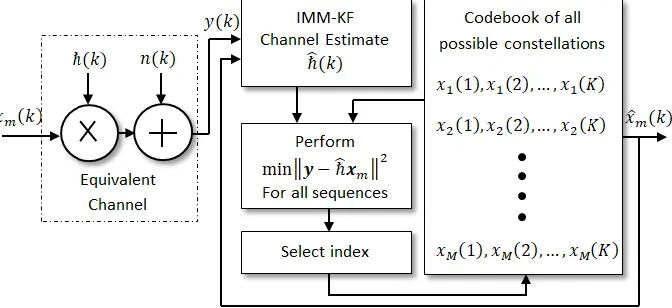
The M-step (25) signifies the most surviving path essential for the MLE algorithm, while it is directly realized by the IMM-KF. The E-step (24) forms the basis to maximize (6) and (7) or minimize (19) and relates to both the IMM-KF and MLE. Fig. 2 shows a block diagram of the proposed AMC system based on the IMM-KF adaptive channel estimation.
As can be seen from Fig. 2, there is one loop involved in the search algorithm performed over all incoming data samples and constellation candidates. Upon discovering a constellation match, the next cycle of channel estimate is thereby directly calculated using the encoded sequence. On the other hand, the MLE algorithm constitutes another loop in addition to the above mentioned one, which is related to the search of best channel estimate as per optimized convex function. Evidently, such interlacing loops of exhaustive search for constellation index and channel estimate could be permissible for small data alphabet size and small data record only. As the data extents get larger, the IMM-KF admirably promises for better convergence as its reckoning load is half of that of the MLE method, as will be seen in the next section.
Fig. 2. Simplified AMC system diagram based on IMM-KF for channel estimate.
IX. COMPLEXITY ANALYSIS
The computational complexity of the proposed IMM-KF for AMC is assessed and compared against the classical MLE approach in this section. In addition to the optimum performance of IMM-KF algorithm, which will be demonstrated in the following simulation exercises, this section is intended to emphasize the main feature of IMM-KF
computational analysis of IMM-KF featuring space reduction for the purpose of AMC implementation is illustrated for the first time in this paper.
Without loss of generality, the complexity of any ACM scheme is proportional with respect to the numbers of code sequence and alphabets. Since the code sequence is assumed intact here, the complexity will hence be governed by the alphabets order only. Further assumptions also need to be considered while facilitating the computational approximations. Firstly, the computations are performed over one data sample; secondly, the eigenvectors are uncorrelated and without inter-modal interference; and thirdly, the channel statistics do not vary.
The computational complexity usually involves the overall operation of mathematical addition, subtraction, multiplication and division procedures. The computational complexity loads of the essential operations 𝒪(. ) for both the IMM-KF and MLE in comparison with other schemes [5, 16] can be easily deduced as shown in Table I below.
TABLE I
COMPUTATIONAL COMPLEXITY FOR COMPLETE EM CYCLE
Item Load Comments
IMM-KF 𝒪(𝑀) FET space reduction
MLE 𝒪(2𝑀) FET space reduction
[5] 𝒪(2𝑁𝑡𝑁𝑟𝑀𝑁𝑡) MIMO without space reduction
[16] 𝒪(2𝑀𝑁𝑡) MIMO with WRD/WLD space reduction
Recall that the subspace is reduced by combining the MRC and SVD algorithms, the classifiers’ complexity can be easily assessed as it is dropped from 𝒪(𝑁𝑡𝑁𝑟𝑀𝑁𝑡) [5] and 𝒪(𝑀𝑁𝑡) [16] to 𝒪(𝑀) for each step in the EM algorithm. The optimal MLE requires 𝒪(𝑀) for each iteration in (24) and (25), while the proposed IMM-KF needs one iteration in (24) only and its estimate can be readily inserted into (25) without extra burdens. Such a complexity reduction result remains the same whether dealing with single or multiple antennas, as per the guidance provided in this paper. The figures of 𝒪(𝑁𝑡𝑁𝑟𝑀𝑁𝑡) and 𝒪(𝑀𝑁𝑡) in reality can grow overly unfeasible for larger constellations and antennas’ aggregates, while the IMM-KF and MLE overheads are fixed and thereby converge easily. The IMM-KF even has half the computational requirements compared to the MLE and, hence, can be advocated for better economical JCEDD enactment in the real-time AMC systems. The superiority of the proposed scalar IMM-KF algorithm using the FET approach for space reduction is tangible; otherwise, the vector computation of KF [10], and hence the resulting IMM, would be tediously high.
X. SIMULATION RESULTS AND DISCUSSION
The performance corroboration of the proposed adaptive IMM-KF estimator is presented using simulation exercises in this section. The innovative paradigm of FET subspace reduction is incorporated in the signal model of 3×3 MIMO
configuration. The signaling is evoked by a BPSK sequence of 129 samples length and unity power sent in the direction of a Rayleigh channel. The channel is assumed with plausible flat fading over certain block samples. An AWGN is also incurred in these channels and the SNR is 10 dB. In each simulation scenario, the 129 samples are divided into three block segments; the length of each is 43 samples, to manifest fixed fading. The segmented channel fading magnitudes along with their corresponding SRSVs are given in Table II. The three segments of the first channel exhibit severe, medium and mild fading behaviors, respectively, while the second channel is assumed to have the opposite behavior. These arbitrary fading attributes are plotted in Fig. 3 and Fig. 4, respectively.
TABLE II
SCENARIO OF (3 × 3 ) MIMO CHANNEL PARAMTERS.
Item MIMO
𝐻 blocks [0.90.9𝑗0.9; 0.9𝑗0.90.9; 𝑗0.9, 0.9, 0.9] [0.50.5𝑗0.5; 0.5𝑗0.50.5; 𝑗0.50.50.5] [0.10.1𝑗0.1; 0.1𝑗0.10.1; 𝑗0.10.10.1]
√𝜆 SRSV [21.271.27] [1.110.70.7] [0.220.140.14]
FET 4.54
2.51 0.5
Fig. 3. SRSVs of block-fading Rayleigh channel in AWGN.
From Fig. 3, it is quite evident that each single path of decomposed channels carries important components of the overall transmission power and hence it is better to be summed rather than being treated individually or merely use the dominant maximum eigenmode for transmission only, which is the case of ET. This is the main concept underlining the meaningful postulation of the new paradigm of FET proposed here. Such an approach consequently keeps as much channel power as possible and maintains an efficient track of its varying conditions, instead of being aborted and vanished to nowhere. The power components of different channel paths have a direct impact on the transmitted signal power and hence it is more advisable to be all consolidated and exploited.
20 40 60 80 100 120
0 0.5 1 1.5 2 2.5
Sequence
M
ag
ni
tu
de
1 2 3
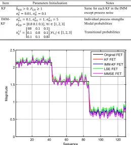
Let us now assess the adaptive CSI estimation of IMM-KF and compare it to a single KF and to the other two conventional estimators, namely; the least-square estimator (LSE) and the minimum mean-square estimator (MMSE). These classical estimators are equivalent to the MLE and maximum a-posteriori estimator (MAPE) under uncorrelated Gaussian noise impairments. The initialization of KF and IMM-KF are assigned values as shown in Table III, while the other estimators do not need such an initialization process. As shown in the table, a 3-KF bank is employed to facilitate the IMM algorithm with initial probabilities of 0.1, 0.8 and 0.1 for each individual filter, while the transitional probabilities of 0.8, 0.1 and 0.1 represent the local, neighbor and remote FSMC states, respectively. Each KF has a single 𝜎𝑤2 value, such as 0.01, 0.1 and 1, to correspond to mild, moderate and severe channel conditions, respectively.
TABLE III
INITIALIZATION OF KF AND IMM-KF ALGORITHMS.
Item Parameters Initialisation Notes
KF ℎ̂0|0> 0, 𝑃1|0≥ 1 𝜎𝑛2= 0.01, 𝜎
𝑤2= 0.1
Same for each KF in the IMM except process noise
IMM-KF
𝜎𝑤12 = 0.1, 𝜎𝑤22 = 1, 𝜎𝑤32 = 5 𝜇0|0𝑖 = [0.80.10.1], ∀𝑖 ∈ [1, 2, 3]
𝜋0𝑖,𝑗= [
08 0.1 0.1 0.1 0.8 0.1 0.1 0.1 0.8
],∀𝑖, 𝑗 ∈ [1, 2, 3]
Individual process strengths Modal probabilities
Transitional probabilities
Fig. 4. Estimation of SRSVs over block-fading Rayleigh channel in AWGN.
The estimators are separately allocated through the given channels and the simulation outcomes are compiled in Fig. 4 for the (3 × 3 ) MIMO transmission scenario. The figure shows that all estimators maintain a good track of the channels’ SRSV variations; yet some perform better than others. The KF and IMM-KF clearly outperform the LSE and MMSE and the IMM-KF is preferred, especially during the channels’ deep fading parts. The IMM-KF is also superior through the channels’ transitions between states, which is inherited from the FSMC’s natural behavior. The main driver behind the IMM-KF’s robust adaptation performance is
centered on the attractive switching competence of the IMM structure itself. If the channel has mild fading, the KF with the lowest state noise power σ𝑤12 = 0.1 is assigned the highest weight in the output of probability combining. As the fade moderates, the state noise power σ𝑤22 = 1 is allocated the next highest weight than other KFs in the IMM bank. The deep fading effect is treated with the highest state noise power
σ𝑤32 = 5 and the output of combining probability receives the highest weight accordingly. The first encounter is similar to the situation of having a lone KF with action virtually reminiscent of a low-pass filter (LPF). This LPF reduces the channels’ harsh fluctuations and smooths out the output as revealed in the two plots.
Moreover, the transitional probabilities of 0.8 and 0.1 represent the percentage of time a state spends for about 80% in its current positions and makes a transition to adjacent cells, whether forward or backward, with 10% likelihood occurrence of each. However, the modal and transitional probabilities change with respect to the innovation behavior of each KF branch as the time elapses. The perspectives of such IMM-KF switching probabilities to cope with the various jumping fades are clearly distinguished in Fig. 5.
Fig. 5. Modal probabilities of 3-bank KFs over block-fading channel.
The remaining simulation exercises are conducted to assess the AMC performance using the proposed IMM-KF and compared to that of MLE and perfectly known channel (KC). The same initialization settings are used again for the IMM-KF structure, but now rather different combinations of antennas are used. A challenging 3-tuple set of nesting constellations {BPSK, 8-PSK, 16-PSK} is generated using the celebrated procedure. The results of 103 Monte Carlo runs over an uncorrelated slow-fading Rayleigh channel and 1 × 1
and 2 × 2 antennas are shown in Figs. 6 and 7, respectively.
The results illustrate the probability of correct classification
𝑃𝐶𝐶 calculated for the IMM-KF, MLE and KC, where the latter serves as an upper performance bound. Table IV shows their correct classification rates at 0 dB.
20 40 60 80 100 120
0 0.5 1 1.5 2 2.5
Sequence
M
ag
ni
tu
de
Original FET KF FET IMM-KF FET LSE FET MMSE FET
20 40 60 80 100 120
0 0.1 0.2 0.3 0.4 0.5 0.6 0.7 0.8 0.9 1
Sequence
M
od
e
P
ro
ba
bi
lit
y
TABLE IV
CORRECT CLASSIFICATION RATES AT 0 dB.
1 × 1 antennas 2 × 2 antennas
KC MLE IMM-KF KC MLE IMM-KF
BPSK 0.99 0.99 0.99 1 1 1
8-PSK 0.85 0.85 0.85 0.98 0.98 0.98
16-PSK 0.57 0.57 0.57 0.75 0.75 0.75
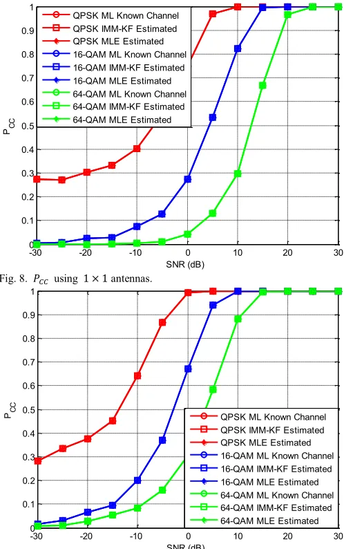
The same simulation scenarios are repeated using another 3-tuple set of different constellations, namely {QPSK, 16-QAM, 64-QAM}, which is tailored to realistic common systems. The ensuing 𝑃𝐶𝐶 trends are depicted in Figs. 8 and 9, for 1 × 1 and
2 × 2 antennas, respectively, and the values of which
calculated at 0 dB are given in Table V below.
TABLE V
CORRECT CLASSIFICATION RATES AT 0 dB.
1 × 1 antennas 2 × 2 antennas
KC MLE IMM-KF KC MLE IMM-KF
QPSK 0.75 0.75 0.75 0.99 0.99 0.99
16-QAM 0.27 0.27 0.27 0.67 0.67 0.67
64-QAM 0.04 0.04 0.04 0.30 0.30 0.30
Fig. 6. 𝑃𝐶𝐶 using 1 × 1 antennas.
Fig. 7. 𝑃𝐶𝐶 using 2 × 2 antennas.
The results show that the proposed IMM-KF performs similarly to the optimal MLE and both coincide with the KC
irrespective of antennas employed. The increased SNR yields for a gradual dominance of the signal covariance matrix and to spread its eigenvalues, which enhances the signal detection accordingly. All methods are also effective in combating the nesting effect to a certain limit, whereas the trends of correct classification are clearly shifting down for larger constellations’ sizes. A classifier to attain correct decisions hence becomes more difficult with the severity of lesser spaces between constellations’ points. Such a demand is very evident in the cases of 16-PSK, 16-QAM and 64-QAM as the spaces between adjacent constellation points becomes more crowded and the detection hence becomes very tasking. For the same 𝑀-ary, the QAM suffers from magnitude and phase variants that are even harder to identify.
Fig. 8. 𝑃𝐶𝐶 using 1 × 1 antennas.
Fig. 9. 𝑃𝐶𝐶 using 2 × 2 antennas.
To show more appreciation for the superiority of complexity saving accredited to the proposed FET for space reduction in comparison with other methods, the next exercise is aimed to accentuate this major advantage. Due to the massive number of resulting operations while increasing the antennas and alphabets spaces, only a limited number of these parameters are considered in the simulation. The trends
-30 -20 -10 0 10 20 30
0 0.1 0.2 0.3 0.4 0.5 0.6 0.7 0.8 0.9 1
SNR (dB) PC
C
BPSK ML Known Channel BPSK IMM-KF Estimated BPSK MLE Estimated 8-PSK ML Known Channel 8-PSK IMM-KF Estimated 8-PSK MLE Estimated 16-PSK ML Known Channel 16-PSK IMM-KF Estimated 16-PSK MLE Estimated
-30 -20 -10 0 10 20 30
0 0.1 0.2 0.3 0.4 0.5 0.6 0.7 0.8 0.9 1
SNR (dB) PC
C
BPSK ML Known Channel BPSK IMM-KF Estimated BPSK MLE Estimated 8-PSK ML Known Channel 8-PSK IMM-KF Estimated 8-PSK MLE Estimated 16-PSK ML Known Channel 16-PSK IMM-KF Estimated 16-PSK MLE Estimated
-30 -20 -10 0 10 20 30
0 0.1 0.2 0.3 0.4 0.5 0.6 0.7 0.8 0.9 1
SNR (dB) PC
C
QPSK ML Known Channel QPSK IMM-KF Estimated QPSK MLE Estimated 16-QAM ML Known Channel 16-QAM IMM-KF Estimated 16-QAM MLE Estimated 64-QAM ML Known Channel 64-QAM IMM-KF Estimated 64-QAM MLE Estimated
-30 -20 -10 0 10 20 30
0 0.1 0.2 0.3 0.4 0.5 0.6 0.7 0.8 0.9 1
SNR (dB) PC
C
depicted in Fig. 10, which are based on the entries of Table I, demonstrate the computational figures using constellation sizes of 2, 4, and 8 and for few transmit antennas 1, 2, and 3, respectively. From Fig. 10 it is clear as the numbers of constellation size and transmit antennas increase, the computational demands increase drastically. For a practical MLE-AMC system employing 64-ary alphabet and 4-MIMO antennas, the computational cost is well anticipated to be in the range of 268.43×10⁶ operations without space reduction and 16.77×10⁶ operations with WRD or WLD space reduction. Such computations increase intensely for massive MIMO and large constellations and become more unbearable in reality, and hence the proposed FET approach provides an attractive alternative choice to produce radical computational savings. One last note concerning Fig. 10 is that the IMM-KF and MLE schemes employing FET perform similarly regardless of the number of antennas. Their computations remain very minimal compared to other channel decompositions aiming at space reduction, and hence one more exercise would be beneficial to reveal the full situation as will be exposed below.
Fig. 10. Number of operations versus constellation size for different antennas.
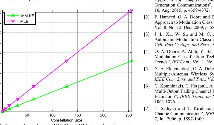
Fig. 11. Number of operations in IMM-KF and MLE, regardless of antennas.
Now, in order to make a distinct differentiation between the IMM-KF and MLE operations using the FET procedure, another exercise is performed and the results of which are depicted in Fig. 11. Based on the entries of Table I, the computational loads for both IMM-KF and MLE featuring FET have a linear relationship with respect to the constellation size. The effectiveness of applying the IMM-KF is very apparent compared to the MLE as it retains only half of the computations required to implement the JCEDD for one complete EM cycle. Reducing the dimensionality by facilitating the FET approach and getting further gain in lowering the computational cost is chiefly accredited to the IMM-KF. Such breakthrough constitutes a corner stone in the design of many mission-critical and tactical systems in reality.
XI. CONCLUSIONS
An efficient AMC paradigm featuring the IMM-KF mixture to elicit a robust and reliable CSI estimate is proposed in this paper. The adaptive IMM-KF estimation is based on decomposing the CSI parameters into a small number of parallel components, by applying the well-known SVD methodology, and then adding up their dominant ETs, which is newly called Frobenius ET (FET) in this paper. This accordingly will maintain the total power of all ETs instead of the waste resulting from relying on individual ETs only. The estimate is applied over Rayleigh MIMO channel and directly admitted to the EM recursion to invoke the Q(HLRT) for AMC core framework. Further to the viable performance, the overall IMM-KF computation is significantly less demanding compared to the optimal MLE especially with large constellation sizes. The IMM-KF only needs one search loop to find the best constellation candidate and is hence more economical than the MLE, which requires two extensive loops to fulfil the EM complete cycle.
REFERENCES
[1] B. Li, S. Li, J. Hou, J. Fu, C. Zhao and A. Nallanathan, “A Bayesian Approach for Adaptively Modulated Signals Recognition in Next-Generation Communications”, IEEE Trans. on Sig. Pro., Vol. 63, No. 16, Aug. 2015, p. 4359-4372.
[2] F. Hameed, O. A. Dobre and D. C. Popescu, “On the Likelihood-Based Approach to Modulation Classification”, IEEE Trans. on Wireless Com., Vol. 8, No. 12, Dec. 2009, p. 5884-5892.
[3] J. L. Xu, W. Su and M. C. Zhou, “Likelihood-Ratio Approaches to Automatic Modulation Classification”, IEEE Trans. on Sys., Man, and
Cyb.-Part C: Apps. and Revs., Vol. 41, No. 4, July 2011, p. 455-469.
[4] O. A. Dobre, A. Abdi, Y. Bar-Ness and W. Su, “Survey of Automatic Modulation Classification Techniques: Classical Approaches and New Trends”, IET Com., Vol. 1, No. 2, 2007, p. 137-156.
[5] Y. A. Eldemerdash, O. A. Dobre and M. Oner, “Signal Identification for Multiple-Antenna Wireless Systems: Achievements and Challenges”,
IEEE Com. Surs. and Tuts., Vol. 18, No. 3, 2016, p. 1524-1551.
[6] C. Komninakis, C. Fragouli, A. H. Sayed and R. D. Wesel, “Multi-Input Multi-Output Fading Channel Tracking and Equalization Using Kalman Estimation”, IEEE Trans. on Sig. Pro., Vol. 50, No. 5, May 2002, p. 1065-1076.
[7] T. Sathyan and T. Kirubarajan, “Markov-Jump-System-Based Secure Chaotic Communication”, IEEE Trans. on Cir. and Sys. -I, Vol. 53, No. 7, Jul. 2006, p. 1597-1609.
2 3 4 5 6 7 8
0 1000 2000 3000 4000 5000 6000 7000 8000 9000 10000
Constellation Size
O
pe
ra
tio
ns
Nt = 1,2,3 FET IMM-KF
Nt = 1,2,3 FET MLE Nt = 1 , [5]
Nt = 2 , [5]
Nt = 3 , [5]
Nt = 1 , [16] Nt = 2 , [16]
Nt = 3 , [16]
7.4 7.6 7.8 8
0 1000 2000 3000
50 100 150 200 250
50 100 150 200 250 300 350 400 450 500
Constellation Size
O
pe
ra
tio
ns
[8] M. R. McKay, A. J. Grant and I. B. Collings, “Performance Analysis of MIMO-MRC in Double-Correlated Rayleigh Environments”, IEEE
Trans. on Com., Vol. 55, No. 3, Mar. 2007, p. 497-507.
[9] L. G. Ordonez, D. P. Palomar and J. R. Fonollosa, “Ordered Eigenvalues of a General Class of Hermitian Random Matrices and Performance Analysis of MIMO Systems”, Proc. ICC, 18-23 May 2008, Beijing, p. 3846-3852.
[10] R. Prasad, C. R. Murthy and B. D. Rao, “Joint Channel Estimation and Data Detection in MIMO-OFDM Systems: A Sparse Bayesian Learning Approach”, IEEE Trans. on Sig. Pro., Vol. 63, No. 20, Oct. 2015, p. 5369-5382.
[11] P. Sadeghi, R. A. Kennedy, P. B. Rapajic and R. Shams, “Finite-State Markov Modeling of Fading Channels: A Survey of Principles and Applications”, IEEE Sig. Pro. Mag., Sep. 2008, p. 57-80.
[12] H. Zhang, S. Wei, G. Ananthaswamy and D. L. Goeckel, “Adaptive Signaling Based on Statistical Characterizations of Outdated Feedback in Wireless Communications”, Proc. of the IEEE, Vol. 95, No. 12, Dec. 2007, p. 2337-2353.
[13] S. H. Ting, K. Sakaguchi and K. Araki, “A Robust and Low Complexity Adaptive Algorithm for MIMO Eigenmode Transmission System with Experimental Validation”, IEEE Trans. on Wireless Com., Vol. 5, No. 7, Jul. 2006, p. 1775-1784.
[14] G. B. Giannakis, Z. Liu, X. Ma and S. Zhou, “Space-Time Coding for
Broadband Wireless Communications”, John Wiley & Sons, 2007.
[15] M. M. Mansour, “A Near-ML MIMO Subspace Detection Algorithm”,
IEEE Sig. Pro. Let., Vol. 22, No. 4, Apr. 2015, p. 408-412.
[16] H. Sarieddeen, M. M. Mansour and A. Chehab, “Modulation Classification via Subspace Detection in MIMO Systems”, IEEE Com. Let., Vol. 21, No. 1, Jan. 2017, p. 64-67.
[17] Y.-C. Liang, K.-C. Chen, G. Y. Li, and P. Mahonen, “Cognitive Radio Networking and Communications: An Overview,” IEEE Trans. Veh. Tech., vol. 60, no. 7, p. 3386-3407, Sep. 2011.
[18] J. J. Popoola and R. van Olst, “A Novel Modulation-Sensing Method”,
IEEE Veh. Tech. Mag., Sep. 2011, p. 60-69.
[19] F. K. Jondral, “Cognitive Radio: A Communications Engineering View”, IEEE Com. Mag., Aug. 2007, p. 28-33.
[20] D. Zhu, V. J. Mathews and D. H. Detienne, “A Likelihood-Based Algorithm for Blind Identification of QAM and PSK Signals”, IEEE
Trans. on Wireless Com., Vol. 17, No. 5, May 2018, p. 3417-3430.
[21] J. Zheng and Y. Lv, “Likelihood-Based Automatic Modulation Classification in OFDM With Index Modulation”, IEEE Trans. on Veh. Tech., Vol. 67, No. 9, Sep. 2018, p. 8192-8204.
[22] M. Abu-Romoh, A. Aboutaleb and Z. Rezki, “Automatic Modulation Classification Using Moments and Likelihood Maximization”, IEEE
Com. Let., Vol. 22, No. 5, May 2018, p. 938-941.
[23] Y. A. Eldemerdash, O. A. Dobre, O. Ureten and T. Yensen, “A Robust Modulation Classification Method for PSK Signals Using Random Graphs”, IEEE Trans. on Ins. and Mea., Vol. 68, No. 2, Feb. 2019, p. 642-644.
[24] F. Meng, P. Chen, L. Wu and X. Wang, “Automatic Modulation Classification: A Deep Learning Enabled Approach”, IEEE Trans. on
Veh. Tech., Vol. 67, No. 11, Nov. 2018, p. 10760-10772.
[25] J. Tian, Y. Pei, Y.-D. Huang and Y.-C. Liang, “Modulation-Constrained Clustering Approach to Blind Modulation Classification for MIMO Systems”, IEEE Trans. on Cog. Com. and Net., Vol. 4, No. 4, Dec. 2018, p. 894-907.
[26] S. Majhi, R. Gupta, W. Xiang and S. Glisic, “Hierarchical Hypothesis and Feature-Based Blind Modulation Classification for Linearly Modulated Signals”, IEEE Trans. on Veh. Tech., Vol. 66, No. 12, Dec. 2017, p. 11057-11069.
[27] J. Zhang, F. Wang, Z. Zhong and S. Wang, “Continuous Phase Modulation Classification via Baum-Welch Algorithm”, IEEE Com. Let., Vol. 22, No. 7, Jul. 2018, p. 1390-1393.
[28] L. Tong and S. Perreau, “Multichannel Blind Identification: From Subspace to Maximum Likelihood Methods”, Proc. of the IEEE, Vol. 86, No.10, 1998, p.1951-1968.
[29] N. Seshadri, “Joint Data and Channel Estimation and Using Blind Trellis Search Techniques”, IEEE Trans. on Com., Vol. 42, No. 2/3/4, Feb/Mar/Apr 1994, p. 1000-1011.
[30] S. Chen and Y. Wu, “Maximum Likelihood Joint Channel and Data Estimation Using Genetic Algorithms”, IEEE Trans. on Sig. Proc., Vol. 46, No. 5, May 1998, p. 1469- 1473.
[31] M. Abuthinien, S. Chen and L. Hanzo, “Semi-Blind Joint Maximum Likelihood Channel Estimation and Data Detection for MIMO Systems”, IEEE Sig. Pro. Let., Vol. 15, 2008, p. 202-205.
[32] O. Bayer and M. Oner, “Joint Space Time Block Code and Modulation Classification for MIMO Systems”, IEEE Wireless Com. Let., Vol. 6, No. 1, Feb. 2017, p. 62-65.
[33] A. Gomaa, L. M. A. Jalloul, M. M. Mansour, K. Gomadam, and D. Tujkovic, “Max-Log-MAP Optimal MU-MIMO Receiver for Joint Data Detection and Interferer Modulation Classification”, IEEE Com. Let., Vol. 20, No. 7, Jul. 2016, p. 1389-1392.
[34] C. Cozzo and B. L. Hughes, “An Adaptive Receiver for Space-Time Trellis Codes Based on Per-Survivor Processing”, IEEE Trans. on Com. Vol. 50, No. 8, Aug. 2002, p. 1213-1216.