Approximate Submodularity and its Applications: Subset
Selection, Sparse Approximation and Dictionary Selection
∗Abhimanyu Das† [email protected] Google
David Kempe‡
[email protected] Department of Computer Science University of Southern California
Editor:Jeff Bilmes
Abstract
We introduce the submodularity ratio as a measure of how “close” to submodular a set functionf is. We show that whenf has submodularity ratioγ, the greedy algorithm for maximizingf provides a (1−e−γ)-approximation. Furthermore, whenγ is bounded away from 0, the greedy algorithm for minimum submodular cover also provides essentially an
O(logn) approximation for a universe ofnelements.
As a main application of this framework, we study the problem of selecting a subset of k random variables from a large set, in order to obtain the best linear prediction of another variable of interest. We analyze the performance of widely used greedy heuristics; in particular, by showing that the submodularity ratio is lower-bounded by the smallest 2k -sparse eigenvalue of the covariance matrix, we obtain the strongest known approximation guarantees for the Forward Regression and Orthogonal Matching Pursuit algorithms.
As a second application, we analyze greedy algorithms for the dictionary selection prob-lem, and significantly improve the previously known guarantees. Our theoretical analysis is complemented by experiments on real-world and synthetic data sets; in particular, we focus on an analysis of how tight various spectral parameters and the submodularity ratio are in terms of predicting the performance of the greedy algorithms.
1. Introduction
Over the past 10–15 years, submodularity has established itself as one of the workhorses of the Machine Learning community. A function f mapping sets to real numbers is called submodular if f(S∪ {v})−f(S) ≥f(T ∪ {v})−f(T) wheneverS ⊆T. One of the most popular consequences of submodularity is that greedy algorithms perform quite well for maximizing the function subject to a cardinality constraint. Specifically, suppose that f is non-negative, monotone, and submodular, and consider the algorithm that, forkiterations,
∗. A preliminary version was included in the proceedings of ICML 2011 under the title “Submodular Meets Spectral: Greedy Algorithms for Subset Selection, Sparse Approximation and Dictionary Selection.” †. Work done while the author was at the University of Southern California, supported in part by NSF
grant DDDAS-TMRP 0540420.
‡. Supported in part by NSF CAREER award 0545855, and NSF grant DDDAS-TMRP 0540420.
c
adds the elementxi+1 that has largest marginal gainf(Si∪ {xi+1})−f(Si) with respect to
the current setSi. By a classic result of Nemhauser et al. (1978), this algorithm guarantees that the final set achieves a function value within a factor 1−1/e of the optimum setS∗ of cardinality k.
This approximation guarantee has been applied in a large number of settings; see, e.g., a survey in (Krause and Golovin, 2014). Of course, greedy algorithms are also popular when the objective function is not submodular. Typically, whenf is not submodular, the greedy algorithm, though perhaps still useful in practice, will not provide theoretical performance guarantees. However, one might suspect that when f is “close to” submodular, then the performance of the greedy algorithm should degrade gracefully.
In the present article (Section 2), we formalize this intuition by defining a measure of “approximate submodularity” which we term submodularity ratio, and denote by γ. We prove that when a function f has submodularity ratio γ, the greedy algorithm gives a (1−e−γ)-approximation; in particular, whenever γ is bounded away from 0, the greedy algorithm guarantees a solution within a constant factor of optimal. We also show that for the complementaryMinimum Submodular Cover problem, where the goal is to find the smallest setS withf(S)≥C for a given valueC, the greedy algorithm gives essentially an
O(logn) approximation when γ is bounded away from 0.
Subset Selection for Regression. To illustrate the usefulness of the approximate sub-modularity framework, we analyze greedy algorithms for the problem of Subset Selection for Regression: select a subset of k variables from a given set of n observation variables which, taken together, “best” predict another variable of interest. This problem has many applications ranging from feature selection, sparse learning and dictionary selection in ma-chine learning, to sparse approximation and compressed sensing in signal processing. From a machine learning perspective, the variables are typically features or observable attributes of a phenomenon, and we wish to predict the phenomenon using only a small subset from the high-dimensional feature space. In signal processing, the variables usually correspond to a collection of dictionary vectors, and the goal is to parsimoniously represent another (output) vector. For many practitioners, the prediction model of choice is linear regression, and the goal is to obtain a linear model using a small subset of variables, to minimize the mean square prediction error or, equivalently, maximize the squared multiple correlation
R2 (Johnson and Wichern, 2002; Miller, 2002).
Thus, we formulate the Subset Selection problem for Regression as follows: Given the (normalized) covariances between n variables Xi (which can in principle be observed) and a variableZ (which is to be predicted), select a subset ofk nof the variablesXi and a linear prediction function of Z from the selected Xi that maximizes the R2 fit. (A formal
definition is given in Section 3.) The covariances are usually obtained empirically from detailed past observations of the variable values.
The above formulation is known (see, e.g., (Das and Kempe, 2008)) to be equivalent to the problem of sparse approximation over dictionary vectors: the input consists of a dictionary of n feature vectors xi ∈ Rm, along with a target vector z ∈ Rm, and the goal
covariances of the previous formulation are then exactly the inner products of the dictionary vectors.1
This problem is NP-hard (Natarajan, 1995), so no polynomial-time algorithms are known to solve it optimally for all inputs. Two approaches are frequently used for ap-proximating such problems: greedy algorithms (Miller, 2002; Tropp, 2004; Gilbert et al., 2003; Zhang, 2008) and convex relaxation schemes (Tibshirani, 1996; Cand`es et al., 2005; Tropp, 2006; Donoho, 2005). For our formulation, a disadvantage of convex relaxation tech-niques is that they do not provide explicit control over the target sparsity level k of the solution; additional effort is needed to tune the regularization parameter.
Greedy algorithms are widely used in practice for subset selection problems; for example, they are implemented in all commercial statistics packages. They iteratively add or remove variables based on simple measures of fit with Z. Two of the most well-known and widely used greedy algorithms are the subject of our analysis: Forward Regression (Miller, 2002) and Orthogonal Matching Pursuit (Tropp, 2004). (These algorithms are defined formally in Section 3).
Our main result is that using the approximate submodularity framework, approximation guarantees much stronger than all previously known bounds can be obtained quite imme-diately. Specifically, we show that the relevant submodularity ratio for the R2 objective is lower-bounded by the smallest (2k)-sparse eigenvalueλmin(C,2k) of the covariance matrix
C of the observation variables. Combined with our general bounds for approximately sub-modular functions, this immediately implies a (1−e−λmin(C,2k))-approximation guarantee for Forward Regression. For Orthogonal Matching Pursuit, a similar analysis leads to a somewhat weaker guarantee of essentially (1−e−λmin(C,2k)2). In a precise sense, our analy-sis thus shows that the less singular C (or its small principal submatrices) are, the “closer to” submodular theR2 objective. Previously, Das and Kempe (2008) had shown thatR2 is truly submodular when there are no “conditional suppressor” variables; however, the latter is a much stronger condition.
Most previous results for greedy subset selection algorithms (e.g., (Gilbert et al., 2003; Tropp, 2004; Das and Kempe, 2008)) had been based on coherence of the input data, i.e., the maximum correlation µbetween any pair of variables. Small coherence is an extremely strong condition, and the bounds usually break down when the coherence isω(1/k). On the other hand, most bounds for greedy and convex relaxation algorithms for sparse recovery are based on a weaker sparse-eigenvalue or Restricted Isometry Property (RIP) condition (Zhang, 2009, 2008; Lozano et al., 2009; Zhou, 2009; Cand`es et al., 2005). However, these results apply to a different objective: minimizing the difference between the actual and estimated coefficients of a sparse vector. Simply extending these results to the subset selection problem adds a dependence on the largest k-sparse eigenvalue and only leads to weak additive bounds.
Dictionary Selection. As a second illustration of the approximate submodularity frame-work, we obtain much tighter theoretical performance guarantees for greedy algorithms for dictionary selection (Krause and Cevher, 2010). In theDictionary Selection problem, we are given starget vectors, and a candidate setV of feature vectors. The goal is to select a set
D⊂V of at mostdfeature vectors, which will serve as adictionary in the following sense. For each of the target vectors, the bestk < d vectors from Dwill be selected and used to achieve a goodR2 fit; the goal is to maximize the averageR2 fit for all of these vectors. (A formal definition is given in Section 4.) The problem of finding a dictionary of basis func-tions for sparse representation of signals has several applicafunc-tions in machine learning and signal processing. Krause and Cevher (2010) showed that greedy algorithms for dictionary selection can perform well in many instances, and proved additive approximation bounds for two specific algorithms, SDSMA and SDSOMP (defined in Section 4). Our approximate
submodularity framework directly yields stronger multiplicative approximation guarantees.
Our theoretical analysis is complemented by experiments comparing the performance of the greedy algorithms and a baseline convex-relaxation algorithm for subset selection on two real-world data sets and a synthetic data set. We also evaluate the submodularity ratio of these data sets and compare it with other spectral parameters: while the input covariance matrices are close to singular, the submodularity ratio actually turns out to be significantly larger.
While the submodularity ratio is always lower-bounded by the smallest (sparse) eigen-value, our experiments reveal that this lower bound can be loose. This happens when there are small (sparse) eigenvalues, but the predictor variable is not badly aligned with their eigenspace. Hence, computing the submodularity ratio explicitly (although it appears com-putationally intensive to do so) can lead to stronger post hoc approximation guarantees. In this context, we also discuss ways in which a more careful analysis of the greedy algorithms allows significantly stronger post hoc approximation guarantees.
Our main contributions can be summarized as follows:
1. We introduce (in Section 2) the notion of the submodularity ratio as a predictor of the performance of greedy algorithms. We show that a submodularity ratio of γ leads to a (1−e−γ)-approximation guarantee for the greedy algorithm for maximum coverage. For the minimum cover probem, we show essentially a logγn approximation guarantee for the greedy algorithm.
2. Using the approximate submodularity framework, in Section 3, we obtain the strongest known theoretical performance guarantees for greedy algorithms for subset selection. In particular, we show that the Forward Regression and OMP algorithms are within a 1−e−γ factor and 1−e−(γ·λmin) factor of the optimal solution, respectively (where theγ and λterms are appropriate submodularity and sparse-eigenvalue parameters).
3. Again using the approximate submodularity framework, in Section 4, we obtain the strongest known theoretical guarantees for algorithms for dictionary selection, im-proving on the results of Krause and Cevher (2010). In particular, we show that the SDSMA algorithm is within a factor λmaxγ (1−1e) of optimal.
1.1 Related and Subsequent Work
We provide an overview of related work both in the context of subset selection (and its variants) and in submodular optimization, as well as a discussion of work that appeared subsequent to the conference version of the present article.
1.1.1 Subset Selection and Sparse Recovery
There has been a lot of related work in the statistics, machine learning and signal processing communities on problems with sparsity constraints (such as sparse recovery, compressed sensing, sparse approximation and feature selection).
In sparse recovery, one is given ann×mdictionaryφofmvectors inRn(wheren < m),
along with another vector y ∈ Rn. It is known that y has some sparse representation in
terms ofkvectors ofφ, up to a small noise term, and the goal is to recover the coefficients
α giveny,φand . There has been a lot of recent interest in greedy and convex relaxation techniques for the sparse recovery problems, both in the noiseless and noisy setting. For L1 relaxation techniques, Tropp (2006) showed conditions based on the coherence (i.e., the maximum correlation between any pair of variables) of the dictionary that guaranteed near-optimal recovery of a sparse signal. In (Cand`es et al., 2005; Donoho, 2005), it was shown that if the target signal is truly sparse, and the dictionary obeys a Restricted Isometry Property (RIP), then L1 relaxation can almost exactly recover the true sparse signal. Other results (Zhao and Yu, 2006; Zhou, 2009) also prove conditions under which L1 relaxation can recover a sparse signal. Though related, the above results are not directly applicable to our subset selection formulation, since the goal in sparse recovery is to recover the true coefficients of the sparse signal, as opposed to our problem of minimizing the prediction error of an arbitrary signal subject to a specified sparsity level.
For greedy sparse recovery, Zhang (2008, 2009) and Lozano et al. (2009) provided condi-tions based on sparse eigenvalues under which Forward Regression and Forward-Backward Regression can recover a sparse signal. As with the L1 results for sparse recovery, the objective function analyzed in these papers is somewhat different from that in our subset selection formulation; furthermore, these results are intended mainly for the case when the predictor variable is truly sparse. Simply extending these results to our problem formulation gives weaker, additive bounds and requires stronger conditions than our results.
The papers by Das and Kempe (2008), Gilbert et al. (2003) and Tropp et al. (2003); Tropp (2004) analyzed greedy algorithms for sparse approximation, which as mentioned previously is equivalent to our subset selection formulation presented in this work. In par-ticular, they obtained a 1 + Θ(µ2k) multiplicative approximation guarantee for the mean square error objective and a 1−Θ(µk) guarantee for the R2 objective, whenever the co-herenceµ of the dictionary is O(1/k). These results are thus weaker than those presented here, since they do not apply to instances with even moderate correlations of ω(1/k).
Other analysis of greedy methods includes the work of Natarajan (1995), which proved a bicriteria approximation bound for minimizing the number of vectors needed to achieve a given prediction error.
ad-ditive approximation guarantees. Since their analysis is for a more general problem than subset selection, applying their results directly to the subset selection problem predictably gives much weaker bounds than those presented in this paper for subset selection. Fur-thermore, even for the general dictionary selection problem, our techniques can be used to significantly improve their analysis of greedy algorithms and obtain tighter multiplicative approximation bounds (as shown in Section 4).
In general, we note that the performance bounds for greedy algorithms derived using the coherence parameter are usually the weakest, followed by those using the Restricted Isome-try Property, then those using sparse eigenvalues, and finally those using the submodularity ratio. (We show an empirical comparison of these parameters in Section 5.)
1.1.2 Submodular Maximization and Curvature
In the context of submodular maximization, the celebrated result of Nemhauser et al. (1978) proved that the greedy algorithm obtained a (1−1/e)-approximation for maximizing any monotone, submodular set function subject to a uniform matroid. The same guarantee was obtained by Calinescu et al. (2011) for an arbitrary matroid constraint, using a continuous variant of the greedy algorithm.
While we are not aware of prior work on defining a notion of how far a function is from being submodular (or analyzing greedy algorithms for such functions), there is a well-known notion of curvature (Conforti and Cornu´ejols, 1984; Vondr´ak, 2010) that captures how far a submodular function is from beingmodular. In particular, thetotal curvatureof a submodular set function is defined asc= 1−minS,j /∈S fSf∅((jj)), wherefS(j) =f(S∪j)−f(S).
(Additional related notions include average curvature and monotonicity ratio; see (Iyer, 2015) for a discussion.) Intuitively c measures how far away f is from being modular, and is equal to 0 if f is modular. Conforti and Cornu´ejols (1984) analyzed the greedy algorithm for submodular maximization in terms of thecparameter, and showed a 1c(1−e−c) approximation for a uniform matroid. The result was extended to an arbitrary matroid by Vondr´ak (2010), and an improved guarantee of (1−c/e) was obtained recently by Sviridenko et al. (2015). Curvature was also used by Iyer et al. (2013) to obtain improved bounds for submodular function approximation, PMAC-learning and submodular minimization.
Another notion of approximate modularity was recently proposed by Chierichetti et al. (2015), who defined a function to be-approximately modular if it satisfies all the modularity requirements to within anadditive error. Chierichetti et al. (2015) analyzed how close (in thel∞ distance) any approximately modular function can be to a modular function.
Note that both the notions of total curvature and approximate modularity are different from the submodularity ratio proposed in this paper, which measures how far a set function is from being submodular.
1.1.3 Subsequent Work
ensemble ofanytime predictors that automatically trade computation time with predictive accuracy. Using the submodularity ratio, the authors provide an approximation guarantee for the performance of their ensemble algorithm. Kusner et al. (2014) analyzed greedy methods for training a tree of classifiers for feature-cost sensitive learning, and show that the objective function for obtaining a cost-sensitive tree of classifiers is approximately sub-modular. Qian et al. (2015) proposed a Pareto optimization approach for subset selection in sparse regression and analyzed the performance of their algorithm using the submodularity ratio.
Most directly following up on our initial work is a recent result of Elenberg et al. (2018) that extends our analysis of greedy algorithms for subset selection from the linear regression setting to arbitrary Generalized Linear Models. The main result is a lower bound on any function’s submodularity ratio in terms of its restricted strong convexity and smoothness parameters, which can then be used to obtain approximation guarantees for greedy feature selection algorithms.
2. Approximate Submodularity
We begin by defining our notion of approximate submodularity, and explaining its rela-tionship with the traditional notion of submodularity. Then, we show that approximation results for greedy algorithms degrade gracefully as the function becomes less and less sub-modular.
2.1 Submodularity Ratio
We introduce the notion of submodularity ratio for a general set function, which captures “how close” to submodular the function is. Let X be a universe of elements, and Let
f : 2X →R+ be a non-negative set function.
Definition 1 (Monotonicity, Submodularity) 1. f is monotone iff f(S) ≤ f(T) whenever S ⊆T.
2. f is submodular ifff(S∪ {x})−f(S)≥f(T ∪ {x})−f(T) whenever S⊆T.
Our definition of the submodularity ratio smoothly interpolates between functions that are submodular and those that are far from so.
Definition 2 (Submodularity Ratio) The submodularity ratio of a monotone function
f with respect to a set U and a parameter k≥1 is
γU,k(f) = min
L⊆U,S:|S|≤k,S∩L=∅ P
x∈Sf(L∪ {x})−f(L)
f(L∪S)−f(L) , (1)
where we define 0/0 := 1. Thus, the submodularity ratio captures how much more f can increase by adding any subsetSof sizektoL, compared to the combined benefits of adding its individual elements to L. That Definition 2 generalizes submodularity is captured by the following proposition.
Proof. First, assume that γU,k ≥1 for allU andk. By choosing k= 2 and S={x, y}in
Equation (1), we obtain thatf(L∪ {x}) +f(L∪ {y})≥f(L∪ {x, y}) +f(L), or, rearranged,
f(L∪ {x})−f(L) ≥ f(L∪ {x, y})−f(L∪ {y}). Now, when we have two sets S and
T = S∪ {x1, x2, . . . , xk}, define Si :=S∪ {x1, . . . , xi} for 0≤i ≤k. Setting L =Si now
gives us thatf(Si∪ {x})−f(Si)≥f(Si+1∪ {x})−f(Si+1). Induction oninow completes
the proof.
Conversely, assume thatf is submodular. In Equation (1), letS={x1, . . . , xk}andSi=
{x1, . . . , xi}, and write a telescoping seriesf(L∪S)−f(L) =Pk−i=01f(L∪Si+1)−f(L∪Si).
By submodularity off, we can bound
f(L∪Si+1)−f(L∪Si) = f(L∪Si∪ {xi+1})−f(L∪Si) ≤ f(L∪ {xi+1})−f(L),
which gives us a lower bound of 1 on the ratio.
Remark 4 The submodularity ratio is defined as a minimum over exponentially many val-ues, and in general, it isNP-hard to compute exactly (more recently, Bai and Bilmes (2018) showed that it cannot be computed in polynomial time in the value oracle model). This is a property it shares with the well-known Restricted Isometry Property (RIP) (Cand`es and Tao, 2005): computing the RIP of a matrix is essentially equivalent to computing the ex-pansion of a graph, yet the guarantees for sparse approximation algorithms are frequently expressed in terms of the RIP.
Whether one can efficiently approximate the submodularity ratio to within non-trivial factors is an interesting open question. Approximating it would allow one to at least derive post hoc approximation guarantees, i.e., to give the user guarantees on the approximation quality for the specific instance that was solved. In the appendix, we discuss some (fairly strong) assumptions under which one can derive non-trivial lower bounds on the submodu-larity ratio.
Typically, rather than computing the submodularity ratio on a given instance, one would use problem-specific insights to derive a priori lower bounds on the submodularity ratio in terms of quantities that are easier to compute exactly or approximately. For example, in the primary application studied here (linear regression), the submodularity ratio is lower-bounded by the (easy to compute) smallest eigenvalue of the covariance matrix, and more tightly bounded by the (not so easy to compute) smallest 2k-sparse eigenvalue of the covari-ance matrix. Recently, Elenberg et al. (2018) showed how to derive similar lower bounds for a more general class of linear objective functions. We anticipate that similar types of bounds can be obtained for other classes of objectives.
2.2 The Greedy Algorithm for Maximum Coverage
Probably the most widely used fact about (monotone) submodular functions is that a simple greedy algorithm approximately optimizes the function subject to a cardinality constraint.2 This is a celebrated result by Nemhauser et al. (1978). Specifically, Nemhauser et al. (1978) analyzed the following algorithm.
Let SNG be the final set Sk returned by the algorithm. The following theorem of Nemhauser et al. (1978) is widely used in the Machine Learning and related communities:
Algorithm 1 The Nemhauser Greedy Algorithm for a non-negative, monotone, and sub-modular set function f on a universeX.
1: Initialize S0=∅.
2: foreach iterationi+ 1 = 1,2, . . . do
3: Let xi+1 ∈ X be an element maximizingf(Si∪ {xi+1}), and set Si+1 =Si∪ {xi+1}. 4: OutputSk.
Theorem 5 (Nemhauser et al. (1978)) The setSNGreturned by the Nemhauser Greedy Algorithm guarantees that f(SNG) ≥(1− 1
e)·f(S
∗
k), where Sk∗ is the set maximizing f(S)
among all size-k sets S.
The centerpiece of our algorithmic analysis is a generalization of Theorem 5 to approx-imately submodular functions.
Theorem 6 Let f be a nonnegative, monotone set function, and OPT be the maximum value of f obtained by any set of size k. Then, the set SNG selected by the Nemhauser Greedy Algorithm has the following approximation guarantee:
f(SNG)≥1−e−γSNG,k(f)
·OPT.
Notice that for submodular functions, becauseγSNG,k(f)≥1, our theorem recovers the
result of Nemhauser et al. (1978) as a special case.
Proof. We carry out the analysis in somewhat more generality than needed here, since most of it will be useful in Section 2.3. Letk be the number of iterations that Algorithm 1 was run, and SNG
i the set of elements greedily chosen in the first iiterations. Let SiNG be
the set of variables chosen by the Nemhauser Greedy Algorithm (Algorithm 1) in the first
i iterations. Define A(i) = f(SiNG)−f(Si−NG1) to be the gain obtained from the variable chosen by the algorithm in iterationi. Then f(SNG) =Pki=1A(j).
For simplicity of notation, we write f(x/S) to denote f({x} ∪S)−f(S), and f(T /S) to denote f(T ∪S)−f(S), for any element x ∈ X and sets S and T. We will also write
γSNG,k to denoteγSNG,k(f).
Let S∗ be some (optimum) set of k∗ variables, achieving a value of (at least) C. Let
Si = S∗ \SiNG. By monotonicity of f and the fact that Si ∪SiNG ⊇ S∗, we have that
f(Si ∪SiNG) ≥ C. We will show that at least one of the x ∈ Si is a good candidate in
iteration i+ 1 of the algorithm. First, the joint contribution of Si, conditioned on the set
SiNG, must be fairly large: f(Si/SiNG) = f(Si ∪SiNG)−f(SiNG) ≥ C−f(SiNG). Using Definition 2, as well as SiNG⊆SNG and |Si| ≤k∗,
X
x∈Si
f(x/SiNG)≥γSNG
i ,|Si|·f(Si/S
NG
i ) ≥ γSNG,k∗·f(Si/SiNG).
Let ˆx∈argmaxx∈Sif(x/SiNG) maximizef(ˆx/SiNG). Then we get that
f(ˆx/SiNG)≥ γSNG,k∗
|Si| ·f(Si/S
NG
i ) ≥
γSNG,k∗
k∗ ·f(Si/S
NG
Since the ˆx above was a candidate to be chosen in iteration i+ 1, and the algorithm chose a variablexi+1 such that f(xi+1/SiNG)≥f(x/SiNG) for all x /∈SiNG, we obtain that
A(i+ 1)≥ γSNG,k∗
k∗ ·f(Si/S
NG
i ) ≥
γSNG,k∗
k∗ ·(C−f(S
NG
i )) ≥
γSNG,k∗
k∗ ·(C− i X
j=1
A(j)).
We will use the above inequality to prove by induction on tthat
C−
t X
i=1
A(i)≤C·(1−γSNG,k∗
k∗ )
t ≤ C·e−γSNG,k∗· t
k∗. (2)
The base case is clearly true for t = 0. Suppose that the inequality is true after t
iterations. Then, at iteration t+ 1, we have
C−
t+1
X
i=1
A(i) =C−
t X
i=1
A(i)−A(t+ 1)
≤C−
t X
i=1
A(i)−γSNG,k∗
k∗ ·(C− t X
i=1
A(i))
= (C−
t+1
X
i=1
A(i))·1−γSNG,k∗
k∗
≤C·1−γSNG,k∗
k∗
t+1
,
thus completing the inductive proof. Using Inequality(2) with k = k∗, t = k− 1 and
C= OPT, we obtain that
f(SNG) =
k X
i=1
A(i) ≥ OPT·1−e−γSNG,k
.
This completes the proof of the approximation guarantee.
Remark 7 As the submodularity ratio goes to 0, the approximation guarantee of Theorem 6 deteriorates and becomes 0 in the limit. This is not surprising: in the limit, the definition does not place any restrictions on the function f. Without any restrictions on f, not only can the greedy algorithm perform arbitrarily poorly, but the same may be true for any efficient algorithm, since f might be a function that is provably hard to approximate to within any non-trivial factor.
2.3 The Greedy Algorithm for Minimum Submodular Cover
The “complementary” problem to submodular function maximization is minimum submod-ular cover, where the goal is to find a smallest setS with f(S) ≥C, a given target value. The name derives from one of the most common instance of submodular functions: coverage functions.3 Here, the elements xcorrespond to sets, and the function value f is the size of the union of the selected sets. In the Maximum Coverage Problem, the goal is to maximize the size of the union by selecting ksets, and in the Minimum Set Cover Problem, the goal is to cover all elements selecting as few sets as possible.
For both problems, the greedy algorithm (Algorithm 1) provides essentially best possible guarantees. The only difference is the termination condition: for maximum coverage, the algorithm is terminated when k sets are selected, while for minimum cover, the algorithm is terminated when all elements (or a given number) have been covered. For the Minimum Set Cover Problem, the greedy algorithm achieves a lnn approximation, which is best possible unlessP=NP. For more general monotone submodular functions, the results are somewhat less clean to express, but are summarized by the following theorem of Wolsey (1982).
Theorem 8 (Theorem 1 of Wolsey (1982)) Let f be nonnegative, monotone and sub-modular, and let n=|X |. For any givenC, let k∗(C) be the size of the smallest setS ⊆V
such thatf(S)≥C. Letkbe the size of the setSNG selected by Algorithm 1 when run until
f(S)≥C. Then,
k≤ 1 + log C
C−f(SNG
k−1)
!!
·k∗(C),
where SNG
k−1 is the set selected by Algorithm 1 after k−1 iterations.
If f is integer valued, then
k≤(1 + log(θ))·k∗,
where θ = maxx∈Xf(x) is the maximum value of the set function obtained by a single
element.
We show that Theorem 8, too, extends gracefully to approximately submodular functions
f.
Theorem 9 Let f be a nonnegative and monotone function, and let n = |X |. For any given C, let k∗(C) be the size of the smallest set S ⊆V such that f(S)≥C. Let k be the size of the set SNG selected by Algorithm 1 when run until f(S)≥C. Then,
k≤1 + 1
γSNG,k∗(C)(f)
·log C
C−f(SNG
k−1)
!
·k∗(C),
where SNG
k−1 is the set selected by Algorithm 1 after k−1 iterations.
Proof. We use the same notation as in the proof of Theorem 6. For notational conve-nience, writek∗ =k∗(C). Letk be the number of iterations taken by Algorithm 1, so that
f(SkNG)≥C and f(Sk−NG1)< C. Thusf(SNG) =Pk
j=1A(j).
Let S∗ be a smallest set (i.e., |S∗|=k∗) with f(S∗) ≥C. Substituting t=k−1 into Equation (2) and solving fork, we obtain that
k≤1 + 1
γSNG,k∗(f)
·log C
C−f(Sk−NG1)
!
·k∗,
as claimed.
As with Wolsey’s result for submodular functions, the bounds can be improved whenf
is integer-valued.
Theorem 10 Assume thatf is integer-valued, in addition to all conditions (and notation) of Theorem 9. Let θ= maxx∈Xf(x) is the maximum value of the set function obtained by
any single element. Then, the number k of elements selected by Algorithm 1 satisfies
k≤1 + 1
γSNG,k∗(C)(f)
·log(C)·k∗(C),
k≤ 1 + 1
γSNG,k∗(C)(f)
log
θ γ∅,k∗(f)
!
·k∗(C).
Proof. The first result follow directly from Theorem 9, because C −f(Sk−NG1) ≥ 1 for integer-valued functions.
For the second result, substitutet= γ k∗
SNG,k∗(f)
·logf(kS∗∗)
into Inequality (2) to obtain
that
C−f(StNG)≤C·e−
γ
SNG,k∗
k∗ ·t ≤ k∗.
Because f is a monotone and integer-valued, f(SNG
i )−f(SNGi−1) ≥ 1 for all remaining
iterations i, and it takes at mostk∗ additional iterations to reach a value of C. Hence,
k≤t+k∗ =
1 + 1
γSNG,k∗(f)
·log(C/k∗)
·k∗ ≤
1 + 1
γSNG,k∗(f)
·log
θ γ∅,k∗(f)
·k∗.
The inequality C/k∗ ≤θ/γ∅,k∗(f) is directly from Definition 2.
The same techniques can be used to obtain the following bicriteria approximation guar-antee below. The bicriteria guarguar-antees are similar in spirit to, for instance, (Krause and Golovin, 2014, Theorem 1.5). We believe that similar results for submodular functions are folklore among researchers, though we are unaware of a reference stating precisely the form we give here.
Theorem 11 For any ∈(0,1), if Algorithm 1 is run untilf(SNG)≥(1−)·C, the size of the set SNG that is returned is at most γ 1
SNG,k∗(f)
Proof. For the proof, simply substitute t= γ 1
SNG,k∗(f)
log(1)·k∗(C) into Inequality (2).
A particularly clean corollary of this theorem is obtained when = 1/e. In that case, we obtain a (1−1/e) approximation by increasing the set size by a factor γ 1
SNG,k∗(f). Thus,
instead of a smooth degradation of the customary (1−1/e) approximation guarantee, we can choose a smooth increase in the size of the set that the greedy algorithm is allowed to select, and thus retain the customary (1−1/e) approximation, even for functions that are only approximately submodular.
3. Subset Selection for Regression
As our first and main application of the approximate submodularity framework, we ana-lyze greedy algorithms for subset selection in regression. The goal in subset selection is to estimate a predictor variable Z using linear regression on a small subset from the set of observation variables X = {X1, . . . , Xn}. We use Var[Xi], Cov[Xi, Xj] and ρ(Xi, Xj)
to denote the variance, covariance and correlation of random variables, respectively. By appropriate normalization, we can assume that all the random variables have expectation 0 and variance 1. The matrix of covariances between theXi and Xj is denoted byC, with entriesci,j = Cov[Xi, Xj]. Similarly, we useb to denote the covariances betweenZ and the Xi, with entriesbi= Cov[Z, Xi]. Formally, theSubset Selectionproblem can now be stated
as follows:
Definition 12 (Subset Selection) Given pairwise covariances among all variables, as well as a parameterk, find a setS ⊂ X of at mostkvariablesXiand a linear predictorZ0= P
i∈SαiXi ofZ, maximizing thesquared multiple correlation(Diekhoff, 2002; Johnson and
Wichern, 2002)
R2Z,S = Var[Z]−E
(Z−Z0)2
Var[Z] .
R2 is a widely used measure for the goodness of a statistical fit; it captures the fraction
of the variance of Z explained by variables inS. Because we assumed Z to be normalized to have variance 1, it simplifies toR2Z,S = 1−E
(Z−Z0)2
.
For a set S, we use CS to denote the submatrix ofC with row and column setS, and
bS to denote the vector with only entries bi for i ∈ S. For notational convenience, we frequently do not distinguish between the index setSand the variables{Xi |i∈S}. Given
the subsetS of variables used for prediction, the optimal regression coefficientsαi are well known to be aS = (αi)i∈S =CS−1·bS (see, e.g., (Johnson and Wichern, 2002)), and hence RZ,S2 =b|SCS−1bS. Thus, the subset selection problem can be phrased as follows: GivenC, b, and k, select a set S of at mostk variables to maximizeR2
Z,S =b|S(C −1
S )bS.4
Many of our results are phrased in terms of eigenvalues of the covariance matrix C and its submatrices. Covariance matrices are positive semidefinite, so their eigenvalues are real
and non-negative (Johnson and Wichern, 2002). We denote the eigenvalues of a positive semidefinite matrix A by λmin(A) = λ1(A) ≤ λ2(A) ≤ · · · ≤ λn(A) = λmax(A). We use
λmin(C, k) = minS:|S|=kλmin(CS) to refer to the smallest eigenvalue of anyk×ksubmatrix of C (i.e., the smallestk-sparse eigenvalue), and similarlyλmax(C, k) = maxS:|S|=kλmax(CS).5
We also use κ(C, k) to denote the largest condition number (the ratio of the largest and smallest eigenvalue) of anyk×k submatrix of C. This quantity is strongly related to the Restricted Isometry Property in (Cand`es et al., 2005). We also useµ(C) = maxi6=j|ci,j|to
denote thecoherence, i.e., the maximum absolute pairwise correlation between theXi vari-ables. Recall theL2 vector and matrix norms: kxk2 =pPi|xi|2, and kAk2 =λmax(A) =
maxkxk2=1kAxk2. We also use kxk0 =|{i|xi 6= 0}|to denote the sparsity of a vector x.
The Rayleigh-Ritz representation for kAk2 is useful in bounding λmin(A), as for any
vectorx, we have λmin(A)≤ kAxk2kxk2 .
The part of a variable Z that is not correlated with the Xi for all i∈S, i.e., the part
that cannot be explained by theXi, is called theresidual (see (Diekhoff, 2002)), and defined
as Res(Z, S) =Z−P
i∈SαiXi.
3.1 Approximate Submodularity of R2
The key insight enabling our analysis is a bound on the submodularity ratio of the R2
function. To avoid notational clutter, when we are specifically concerned with the R2
objective defined on the variables Xi, we omit the function name in the definition of the submodularity ratio, and simply write
γU,k = min
L⊆U,S:|S|≤k,S∩L=∅ P
i∈S(R2Z,L∪{Xi}−R2Z,L) R2
Z,S∪L−RZ,L2
= min
L⊆U,S:|S|≤k,S∩L=∅
(bL S)|bLS
(bLS)|(CL S)−1bLS
,
where CL and bL are the normalized covariance matrix and normalized covariance vector
corresponding to the set {Res(X1, L),Res(X2, L), . . . ,Res(Xn, L)}.
Our key lemma can now be stated as follows:
Lemma 13 γU,k≥λmin(C, k+|U|)≥λmin(C).
For all our analysis in this paper, we will use |U| = k, and hence γU,k ≥ λmin(C,2k).
Thus, the smallest 2k-sparse eigenvalue is a lower bound on this submodularity ratio; as we show later, it is often a weak lower bound.
Before proving Lemma 13, we first introduce two lemmas that relate the eigenvalues of a normalized covariance matrix with those of its submatrices.
Lemma 14 LetCbe the covariance matrix ofnzero-mean random variablesX1, X2, . . . , Xn,
each of which has variance at most 1. Let Cρ be the corresponding correlation matrix of
the n random variables, that is, Cρ is the covariance matrix of the variables after they are normalized to have unit variance. Thenλmin(C)≤λmin(Cρ).
Proof. SinceCρis obtained by normalizing the variables such that they have unit variance,
we getCρ=D|CD, where Dis a diagonal matrix with diagonal entries di= √ 1
Var[Xi].
Since both Cρ and C are positive semidefinite, we can perform Cholesky factorization
to get lower-triangular matrices Aρ and A such that C = AA| and Cρ = AρA|ρ. Hence Aρ=D|A.
Letσmin(A) andσmin(Aρ) denote the smallest singular values ofAandAρ, respectively.
Also, letv be the singular vector corresponding toσmin(Aρ). Then,
kAvk2=kD−1Aρvk2 ≤ kD−1k2kAρvk2 = σmin(Aρ)kD−1k2 ≤ σmin(Aρ),
where the last inequality follows since
kD−1k2 = max
i
1
di = maxi p
Var[Xi] ≤ 1.
Hence, by the Courant-Fischer theorem,σmin(A)≤σmin(Aρ), and consequently,λmin(C)≤
λmin(Cρ).
Lemma 15 Letλmin(C)be the smallest eigenvalue of the covariance matrixCof nrandom
variablesX1, X2, . . . , Xn, andλmin(C0)be the smallest eigenvalue of the(n−1)×(n−1)
co-variance matrixC0corresponding to then−1random variablesRes(X1, Xn), . . . ,Res(Xn−1, Xn).
Then λmin(C)≤λmin(C0).
Proof. Letλi andλ0idenote the eigenvalues ofCandC0, respectively. Also, letc0i,j denote the entries ofC0. Using the definition of the residual, we get that
c0i,j = Cov[Res(Xi, Xn),Res(Xj, Xn)] = ci,j−ci,ncj,n
cn,n ,
c0i,i = Var[Res(Xi, Xn)] = ci,i− c
2
i,n cn,n .
DefiningD= cn,n1 ·[c1,n, c2,n, . . . , cn−1,n]|·[c1,n, c2,n, . . . , cn−1,n], we can write C{1,...,n−1}= C0+D. To proveλ1 ≤λ01, lete0 = [e01, . . . , e0n−1]|be the eigenvector ofC0 corresponding to
the eigenvalue λ01, and consider the vector e= [e01, e02, . . . , e0n−1,−cn,n1 Pn−i=11e0ici,n]|. Then,
C·e= [y0], where
y=− 1
cn,n n−1
X
i=1
e0ici,n[c1,n, c2,n, . . . , cn−1,n]|+C{1,...,n−1}·e0
=− 1
cn,n n−1
X
i=1
e0ici,n[c1,n, c2,n, . . . , cn−1,n]|+D·e0+C0·e0
=C0·e0.
Thus, C·e = [λ01e01, λ10e02, . . . , λ01e0n−1,0]| = λ01[e01, e02, . . . , e0n−1,0]| ≤ λ01kek2, which by
Rayleigh-Ritz bounds implies thatλ1≤λ01.
Proof of Lemma 13. Since
(bLS)|(CSL)−1bLS
(bLS)|bL S
≤max
x
x|(CSL)−1x
x|x = λmax((C
L S)
−1) = 1
λmin(CSL)
,
we can use Definition 2 to obtain that
γU,k≥ min
(L⊆U,S:|S|≤k,S∩L=∅)λmin(C
L S).
Next, we relate λmin(CSL) with λmin(CL∪S), using repeated applications of Lemmas 14
and 15. Let L = {X1, . . . , X`}; for each i, define Li = {X1, . . . , Xi}, and let C(i) be the
covariance matrix of the random variables {Res(X, L\Li) | X ∈ S ∪Li}, and Cρ(i) the
covariance matrix after normalizing all its variables to unit variance. Then, Lemma 14 implies that for each i, λmin(C(i)) ≤ λmin(Cρ(i)), and Lemma 15 shows that λmin(Cρ(i)) ≤ λmin(C(i−1)) for each i > 0. Combining these inequalities inductively for all i, we obtain
that
λmin(CSL) =λmin(Cρ(0)) ≥ λmin(C(`)) = λmin(CL∪S) ≥ λmin(C,|L∪S|).
Finally, since|S| ≤kand L⊆U, we obtainγU,k≥λmin(C, k+|U|).
3.2 Forward Regression
We now use our approximate submodularity framework along with the result of Lemma 13 to achieve theoretical performance bounds for Forward Regression and Orthogonal Matching Pursuit, which are widely used in practice. We also analyze the Oblivious algorithm, one of the simplest greedy algorithms for subset selection. Throughout the remainder of this section, we use OPT = maxS:|S|=kR2Z,S to denote the optimumR2 value achievable by any
set of sizek.
We begin with an analysis of Forward Regression, which is the standard algorithm used by many researchers in medical, social, and economic domains.6
Algorithm 2 The Forward Regression (also called Forward Selection) algorithm.
1: Initialize S0=∅.
2: foreach iterationi+ 1 = 1,2, . . . do
3: Let Xi+1 be a variable maximizingR2Z,Si∪{Xi+1}, and setSi+1=Si∪ {Xi+1}. 4: OutputSk.
Notice that Forward Regression is exactly the special case of the general Nemhauser Greedy Algorithm (Algorithm 1) applied to theR2 objective.
Our main result is the following theorem.
Theorem 16 The set SFRselected by Forward Regression has the following approximation guarantees:
R2Z,SFR ≥(1−e −γ
SFR,k)·OPT
≥(1−e−λmin(C,2k))·OPT
≥(1−e−λmin(C,k))·Θ((1 2)
1/λmin(C,k))·OPT.
The first inequality is just an application of Theorem 6 to the R2 objective, and the second inequality follows directly from Lemma 13 by noticing that |SFR| = k. Thus, our proof will focus on the third inequality, which relates the performance measured with respect to the smallestk-sparse eigenvalue to that measured with respect to the smallest 2k-sparse eigenvalue. We begin with a general lemma that bounds the amount by which theR2 value of a set and the sum ofR2 values of its elements can differ.
Lemma 17 Let C and b be the covariance matrix and covariance vector corresponding to a predictor variable Z and a setS of random variables X1, X2, . . . , Xn that are normalized
to have zero mean and unit variance. Then,
1
λmax(C)
n X
i=1
R2Z,Xi ≤R2Z,{X1,...,Xn} ≤ 1
γ∅,n n X
i=1
R2Z,Xi ≤ 1
λmin(C)
n X
i=1
R2Z,Xi.
Proof. Let the eigenvalues ofC−1beλ01≤λ02 ≤. . .≤λ0n, with corresponding orthonormal eigenvectorse1,e2, . . . ,en. We write b in the basis{e1,e2, . . . ,en} asb=Piβiei. Then,
R2Z,{X1,...,Xn} = b|C−1b = X
i β2iλ0i.
Because λ01 ≤λ0i for all i, we get λ01P
iβi2 ≤ R2Z,{X1,...,Xn}, and P
iβi2 =b|b = P
iR2Z,Xi,
because the length of the vector b is independent of the basis it is written in. Also, by definition of the submodularity ratio, R2Z,{X1,...,Xn} ≤
P
iβi2
γ∅,n . Finally, becauseλ 0
1= λmax1(C),
and using Lemma 13, we obtain the result.
The next lemma relates the optimal R2 value using kelements to the optimal R2 using
k0 < k elements.
Lemma 18 For each k, let Sk∗∈argmax|S|≤kR2
Z,S be an optimal subset of at most k
vari-ables. Then, for any k0 = Θ(k) such that λmin1(C,k) < k0 < k, we have that RZ,S2 ∗
k0
≥R2Z,S∗
k
·
Θ((kk0)1/λmin(C,k)), for large enoughk. In particular, R2Z,S∗
k/2
≥R2Z,S∗
k·Θ((
1 2)
1/λmin(C,k)), for
large enough k.
Proof. We first prove that R2Z,S∗
k−1 ≥ (1−
1
kλmin(C,k))R 2
Z,S∗
k. Let T = Res(Z, S ∗
k); then,
Cov[Xi, T] = 0 for allXi ∈S∗k, andZ =T+P Xi∈S∗
kαiXi, whereα= (αi) =C −1
the optimal regression coefficients. We write Z0 =Z −T. For any Xj ∈ Sk∗, by definition
of R2, we have that
R2Z0,S∗
k\{Xj} = 1−
α2jVar[Xj]
Var[Z0] = 1−
α2j
Var[Z0];
in particular, this implies thatR2Z0,S∗
k−1
≥1− α
2 j
Var[Z0] for all Xj ∈Sk∗.
Focus now on j minimizing α2j, so that α2j ≤ kαk22
k . As in the proof of Lemma 17, by
writing α in terms of an orthonormal eigenbasis of CS∗k, one can show that |α|CSk∗α| ≥
kαk2
2λmin(CS∗
k), orkαk
2 2≤
|α|C
S∗
kα|
λmin(CS∗
k)
. Furthermore,α|C
S∗
kα= Var[ P
Xi∈S∗
kαiXi] = Var[Z 0],
soR2Z0,S∗
k−1 ≥1−
1
kλmin(CS∗
k)
. Finally, by definition, R2Z0,S∗
k = 1, so
R2Z,S∗
k−1
R2Z,S∗
k
≥
R2Z0,S∗
k−1
R2Z0,S∗
k
≥ 1− 1
kλmin(CS∗
k)
≥ 1− 1
kλmin(C, k)
.
Now, applying this inequality repeatedly, we get
R2Z,S∗
k0
≥R2Z,S∗
k·
k Y
i=k0+1
(1− 1
iλmin(C, i)
).
Lett=d1/λmin(C, k)e, so that the previous bound impliesR2Z,S∗
k0
≥R2Z,S∗
k·
Qk
i=k0+1 i−ti .
Most of the terms in the product telescope, giving us a bound ofR2Z,S∗
k
·Qti=1 k0−t+i
k−t+i. Since Qt
i=1k 0−t+i
k−t+i converges to ( k0
k)t with increasingk (keepingt constant), we get that for large k,
R2Z,S∗
k0 ≥R
2
Z,Sk∗·Θ(( k0
k)
t) ≥ R2
Z,S∗k·Θ(( k0
k)
1/λmin(C,k)).
This completes the proof.
Using the above lemmas, we now prove the main theorem.
Proof of Theorem 16. As mentioned earlier, the first inequality is a direct corollary of Theorem 6, obtained by replacing f with the R2 function. The second inequality follows directly from Lemma 13 and the fact that|SFR|=k.
By applying the above result after k/2 iterations, we obtainR2Z,SNG k/2
≥(1−e−λmin(C,k))· R2
Z,S∗
k/2. Now, using Lemma 18 and monotonicity ofR
2, we get
R2Z,SNG k
≥ R2Z,SNG k/2
≥ (1−e−λmin(C,k))·Θ((1 2)
1/λmin(C,k))·R2
Z,Sk∗,
Algorithm 3 The Orthogonal Matching Pursuit algorithm.
1: Initialize S0=∅.
2: foreach iterationi+ 1 = 1,2, . . . do
3: LetXi+1be a variable maximizing|Cov[Res(Z, Si), Xi+1]|, and setSi+1=Si∪{Xi+1}. 4: OutputSk.
3.3 Orthogonal Matching Pursuit
The second greedy algorithm we analyze is Orthogonal Matching Pursuit (OMP), frequently used in signal processing domains.
By applying similar techniques as in the previous section, we can also obtain approxi-mation bounds for OMP. We start by proving the following lemma that lower-bounds the variance of the residual of a variable.
Lemma 19 Let A be the (n+ 1)×(n+ 1) covariance matrix of the normalized variables
Z, X1, X2, . . . , Xn. Then Var[Res(Z,{X1, . . . , Xn})]≥λmin(A).
Proof. The matrixA is of the formA=
1 b|
b C
. We useA[i, j] to denote the matrix
obtained by removing the ith row andjth column of A, and similarly forC. Recalling that the (i, j) entry of C−1 is (−1)i+jdet(det(C)C[i,j]), and developing the determinant ofA by the first row and column, we can write
det(A) =
n+1
X
j=1
(−1)1+ja1,jdet(A[1, j])
= det(C) +
n X
j=1
(−1)jbjdet(A[1, j+ 1])
= det(C) +
n X
j=1
(−1)jbj n X
i=1
(−1)i+1bidet(C[i, j])
= det(C)−
n X
j=1
n X
i=1
(−1)i+jbibjdet(C[i, j]) = det(C)(1−b|C−1b).
Therefore, using that Var[Z] = 1,
Var[Res(Z,{X1, . . . , Xn})] = Var[Z]−b|C−1b =
det(A) det(C).
Because det(A) =Qni=1+1λAi and det(C) =Qni=1λCi , andλA1 ≤λC1 ≤λA2 ≤λC2 ≤. . .≤λAn+1
by the eigenvalue interlacing theorem, we get that det(det(AC)) ≥λA1, proving the lemma.
Theorem 20 The set SOMP selected by orthogonal matching pursuit has the following ap-proximation guarantees:
R2Z,SOMP ≥(1−e
−(γSOMP,k·λmin(C,2k)))·OPT
≥(1−e−λmin(C,2k)2)·OPT
≥(1−e−λmin(C,k)2)·Θ((1 2)
1/λmin(C,k))·OPT.
Proof. We begin by proving the first inequality. Using notation similar to that in the proof of Theorem 16, we letSk∗ be the optimum set ofkvariables,SiOMP the set of variables chosen by OMP in the first iiterations, and Si =Sk∗\SiOMP. For each Xj ∈Si, let Xj0 =
Res(Xj, SiOMP) be the residual ofXj conditioned onSiOMP, and writeSi0 ={Xj0 |Xj ∈Si}. Consider some iteration i+ 1 of OMP. We will show that at least one of the Xi0 is a good candidate in this iteration. Let`maximizeR2
Z,X0
`
, i.e.,`∈argmax(j:X0
j∈Si0)R
2
Z,X0
j. By
Lemma 19,
Var[X`0]≥λmin(CSi
G∪{X
0
`}) ≥ λmin(C,2k).
The OMP algorithm chooses a variableXmto add which maximizes|Cov[Res(Z, SiG), Xm]|. Thus,Xm maximizes
Cov[Res(Z, SGi ), Xm]2= Cov[Z,Res(Xm, SGi )]2 = R2Z,Res(Xm,Si
G)
·Var[Res(Xm, SGi )].
In particular, this implies
R2Z,Res(Xm,Si
G)
≥R2Z,X0
`·
Var[X`0] Var[Res(Xm, SGi )]
≥R2Z,X0
`·
λmin(C,2k)
Var[Res(Xm, SGi )] ≥ R
2
Z,X0
`·λmin(C,2k),
because Var[Res(Xm, SGi )]≤1. As in the proof of Theorem 6,R2Z,X`0 ≥
γSOMP,k
k ·R
2
Z,Si0, so
RZ,2 Res(Xm,Si
G)
≥R2Z,S0
i
·λmin(C,2k)·γSOMP,k
k . With the same definition of A(i) as in the proof
of Theorem 6, we get thatA(i+ 1)≥ λmin(C,2k)γSOMP,k
k ·(OPT−
Pi
j=1A(j)). An inductive
proof now shows that
R2Z,SG =
k X
i=1
A(i) ≥ (1−e−λmin(C,2k)·γSOMP,k)·R2 Z,S∗
k.
The proofs of the other two inequalities follow the same pattern as the proof for Forward Regression.
3.4 Oblivious Algorithm
As a baseline, we also consider a greedy algorithm which completely ignores C and simply selects thek variables individually most correlated withZ.
Algorithm 4 The oblivious algorithm.
1: Sort the Xi by non-increasingbi values.
2: Return {X1, X2, . . . , XK}.
Theorem 21 The set SOBL selected by the oblivious algorithm has the following approxi-mation guarantees:
R2Z,SOBL ≥
γ∅,k λmax(C, k)
·OPT ≥ λmin(C, k)
λmax(C, k)
·OPT.
Proof. Let S be the set chosen by the oblivious algorithm, and Sk∗ the optimum set of
k variables. By definition of the oblivious algorithm,P
i∈SR2Z,Xi ≥ P
i∈S∗
kR
2
Z,Xi, so using
Lemma 17, we obtain that
R2Z,S ≥
P
i∈SR2Z,Xi λmax(C, k)
≥
P i∈S∗
kR
2
Z,Xi
λmax(C, k)
≥ γ∅,k
λmax(C, k)
RZ,S2 ∗
k.
The second inequality of the theorem follows directly from Lemma 13.
4. Dictionary Selection Bounds
To demonstrate the wider applicability of the approximate submodularity framework, we next obtain a tighter analysis for two greedy algorithms for the dictionary selection problem, introduced by Krause and Cevher (2010).
The Dictionary Selection problem generalizes the Subset Selection problem by consider-ingspredictor variablesZ1, Z2, . . . , Zs. The goal is to select a dictionaryDofdobservation
variables, to optimize the averageR2 fit for the Zi using at mostkvectors fromDfor each. Formally, the Dictionary Selection problem is defined as follows:
Definition 22 (Dictionary Selection) Given all pairwise covariances among theZj and
Xi variables, as well as parameters d and k, find a set D of at most d variables from
{X1, . . . , Xn} maximizing
F(D) =
s X
j=1
max
S⊂D,|S|=kR
2
Zj,S.
4.1 The Algorithm SDSMA
The SDSMA algorithm generalizes the oblivious greedy algorithm to the problem of
Dic-tionary Selection. It replaces the R2Zj,S term in Definition 22 with its modular approxi-mation f(Zj, S) =
P
i∈SR2Zj,Xi. Thus, it greedily tries to maximize the function ˆF(D) = Ps
j=1maxS⊂D,|S|=kf(Zj, S), over sets D of size at most d; the inner maximum can be
computed efficiently using the oblivious algorithm.
Algorithm 5 TheSDSMA algorithm for dictionary selection.
1: Initialize D0 =∅.
2: foreach iterationi+ 1 = 1,2, . . . do
3: Let Xi+1 be a variable maximizing ˆF(D∪ {Xm}), and set Si+1 =Si∪ {Xi+1}. 4: OutputDd.
Theorem 23 Let DMA be the dictionary selected by the SDSMA algorithm, and D∗ the optimum dictionary of size |D| ≤d, with respect to the objective F(D) from Definition 22. Then,
F(DMA)≥ γ∅,k
λmax(C, k)
(1−1
e)·F(D
∗
) ≥ λmin(C, k)
λmax(C, k)
(1− 1
e)·F(D
∗
).
Proof. Let ˆD be a dictionary of sizedmaximizing ˆF(D). Becausef(Zj, S) is monotone and modular inS, ˆF is a monotone, submodular function. Hence, using the submodularity results of Nemhauser et al. (1978) and the optimality of ˆD for ˆF,
ˆ
F(DMA)≥Fˆ( ˆD)·(1−1
e) ≥ Fˆ(D
∗
)·(1−1
e).
Now, by applying Lemma 17 for eachZj, it is easy to show that ˆF(D∗)≥γ∅,k·F(D∗), and
similarly ˆF(DMA)≤λmax(C, k)·F(DMA). Thus we get F(DMA)≥
γ∅,k
λmax(C,k)(1− 1 e)F(D
∗).
The second part now follows from Lemma 13.
Note that these bounds significantly improve the previous additive approximation guarantee obtained by Krause and Cevher (2010): F(DMA) ≥ (1− 1
e)·F(D
∗)−(2− 1
e)·k·µ(C).
In particular, when µ(C) > Θ(1/k), i.e., even just one pair of variables has moderate correlation, the approximation guarantee of Krause and Cevher becomes trivial.
4.2 The Algorithm SDSOMP
We also obtain a multiplicative approximation guarantee for the greedy SDSOMPalgorithm,
introduced by Krause and Cevher for dictionary selection. Our bounds for SDSOMP are
much stronger than the additive bounds obtained by Krause and Cevher. However, for both our results and theirs, the performance guarantees for SDSOMP are much weaker than
those for SDSMA.
The SDSOMPalgorithm generalizes the Orthogonal Matching Pursuit algorithm for
sub-set selection to the problem of dictionary selection. In each iteration, it adds a new element to the currently selected dictionary by using Orthogonal Matching Pursuit to approximate the estimation of max|S|=kR2Zj,S.
We now show how to obtain a multiplicative approximation guarantee for SDSOMP.
Algorithm 6 TheSDSOMP algorithm for dictionary selection.
1: Initialize D0 =∅.
2: foreach iterationi+ 1 = 1,2, . . . do
3: Let Xi+1 be a variable maximizing Psj=1R2Zj,SOMP(Di∪{Xi+1},Zj,k) where
SOMP(D, Z, k) denotes the set selected by Orthogonal Matching Pursuit for
predicting Z using k variables fromD.
4: SetSi+1=Si∪ {Xi+1}. 5: OutputDd.
Theorem 23.
F(D) =
s X
j=1
max
S⊂D,|S|=kR
2
Zj,S,
ˆ
F(D) =
s X
j=1
max
S⊂D,|S|=kf(Zj, S),
˜
F(D) =
s X
j=1
R2Zj,SOMP(D,Zj,k).
We first prove the following lemma about approximating the function ˆF(D) by ˜F(D):
Lemma 24 For any setD, we have that
(1−e−λmin(C,2k)2)
λmax(C, k)
·Fˆ(D)≤F˜(D) ≤ Fˆ(D)
γ∅,k .
Proof. Using Theorem 20 and Lemma 17 and summing up over all the Zj terms, we obtain that
˜
F(D)≥(1−e−λmin(C,2k)2)·F(D) ≥ (1−e−λmin(C,2k)2) Fˆ(D)
λmax(C, k)
.
Similarly, using Lemma 17 and the fact that maxS⊂D,|S|=kR2Zj,S ≥R2Zj,SOM P(D,Zj,k), we
have
ˆ
F(D)≥γ∅,k·F(D) ≥ γ∅,k·F˜(D).
Using the above lemma, we now prove the following bound for SDSOMP:
Theorem 25 Let DOMP be the dictionary selected by the SDS
OMP algorithm, andD∗ the optimum dictionary of size |D| ≤d, with respect to the objective F(D) from Definition 22. Then,
F(DOMP)≥F(D∗)· γ∅,k
λmax(C, k)
· (1−e
−(p·γ∅,k))
d−d·p·γ∅,k+ 1 ≥ F(D
∗)· λmin(C, k)
λmax(C, k)
· (1−e
−(p·γ∅,k)) d−d·p·γ∅,k+ 1,
Proof. Let ˆD be the dictionary of size d that maximizes ˆF(D). We first prove that ˆ
F(DOMP) is a good approximation to ˆF( ˆD).
Let SNGi be the variables chosen by SDSOMP after i iterations. Define Si = ˆD\SiNG.
By monotonicity of ˆF, we have that ˆF(Si∪SiNG)≥Fˆ( ˆD).
Let ˆX ∈ Si be the variable maximizing ˆF(SiNG ∪ {Xˆ}), and similarly ˜X ∈ Si be the
variable maximizing ˜F(SNG
i ∪ {X˜}).
Since ˆF is a submodular function, it is easy to show (using an argument similar to the
proof of Theorem 16) that ˆF(SiNG∪ {Xˆ})−Fˆ(SiNG)≥ Fˆ( ˆD)−Fˆ(SiNG)
d .
Now, using Lemma 24 above, and the optimality of ˜X for ˜F(SiNG ∪ {X˜}), we obtain that
1
γ∅,k
·Fˆ(SiNG∪ {X˜})≥F˜(SNGi ∪ {X˜}) ≥ F˜(SNGi ∪ {Xˆ}) ≥ p·Fˆ(SiNG∪ {Xˆ}).
Thus, ˆF(SiNG∪ {X˜})≥p·γ∅,k·Fˆ(SiNG∪ {Xˆ}), or
ˆ
F(SiNG∪ {X˜})−Fˆ(SiNG)≥p·γ∅,k·( ˆF(SiNG∪ {Xˆ})−Fˆ(SiNG))−(1−p·γ∅,k) ˆF(SiNG).
Define A(i) = ˆF(SiNG)−Fˆ(Si−NG1) to be the gain, with respect to ˆF, obtained from the variable chosen by SDSOMP in iteration i. Then ˆF(DOMP) = Pdi=1A(i). From the
preceding paragraphs, we obtain
A(i+ 1)≥ p·γ∅,k
d ·( ˆF( ˆD)−(1 + d p·γ∅,k
−d)
i X
j=1
A(j)).
Since the above inequality holds for each iteration i = 1,2, . . . , d, a simple inductive proof shows that
ˆ
F( ˆD)−
d X
i=1
A(i)≤Fˆ( ˆD)·(1−pγ∅,k
d )
d+ (d−dpγ ∅,k)·
d X
i=1
A(i).
Rearranging the terms and simplifying, we get that
ˆ
F(DOMP) =
d X
i=1
A(i) ≥ Fˆ( ˆD)·(1−e
−(p·γ∅,k)) d−dpγ∅,k+ 1
≥ Fˆ(D∗)·(1−e
−(p·γ∅,k)) d−dpγ∅,k+ 1 ,
where the last inequality is due to the optimality of ˆDfor ˆF.
Now, using Lemma 17 for eachZj term, it can be easily seen that ˆF(D∗)≥γ∅,k·F(D∗).
Similarly, using Lemma 3.3 on the setDOMP, we have F(DOMP)≥ 1
λmax(C,k)·Fˆ(DOMP).
Using the above inequalities, we therefore get the desired bound
F(DOMP)≥F(D∗)· γ∅,k
λmax(C, k)
· (1−e
−(p·γ∅,k)) d−d·p·γ∅,k+ 1
.
5. Experiments
In this section, we evaluate Forward Regression (FR) and OMP empirically, on two real-world and one synthetic data set. We compare the two algorithms against an optimal solution (OPT), computed using exhaustive search, the oblivious greedy algorithm (OBL), and the L1-regularization/Lasso (L1) algorithm (in the implementation of Koh et al. (2008)). Beyond the algorithms’ performance, we also compute the various spectral parameters from which we can derive lower bounds. Specifically, these are
1. the submodularity ratio: γSFR,k, where SFR is the subset selected by forward
regres-sion.
2. the smallest sparse eigenvaluesλmin(C, k) andλmin(C,2k). (In some cases, computing
λmin(C,2k) was not computationally feasible due to the problem size.)
3. the sparse inverse condition number κ(C, k)−1. As mentioned earlier, the sparse
in-verse condition numberκ(C, k) is strongly related to the Restricted Isometry Property in (Cand`es et al., 2005).
4. the smallest eigenvalueλmin(C) =λmin(C, n) of the entire covariance matrix.
The aim of our experiments is twofold: First, we wish to evaluate which among the submodular and spectral parameters are good predictors of the performance of greedy al-gorithms in practice. Second, we wish to highlight how the theoretical bounds for subset selection algorithms reflect on their actual performance. Our analytical results predict that Forward Regression should outperform OMP, which in turn outperforms Oblivious. For Lasso, it is not known whether strong multiplicative bounds, like the ones we proved for Forward Regression or OMP, can be obtained.
5.1 Data Sets
Because several of the spectral parameters (as well as the optimum solution) areNP-hard to compute, we restrict our experiments to data sets withn≤30 features, from whichk≤8 are to be selected. We stress that the greedy algorithms themselves are very efficient, and the restriction on data set sizes is only intended to allow for an adequate evaluation of the results.
Each data set containsm > nsamples, from which we compute the empirical covariance matrix (analogous to the Gram matrix in sparse approximation) between all observation variables and the predictor variable; we then normalize it to obtainC and b. We evaluate the performance of all algorithms in terms of their R2 fit; thus, we implicitly treat C and
b as the ground truth, and also do not separate the data sets into training and test cases. Our data sets are the Boston Housing Data, a data set of World Bank Development Indicators, and a synthetic data set generated from a distribution similar to the one used by Zhang (2008). The Boston Housing Data (available from the UCI Machine Learning Repository) is a small data set frequently used to evaluate ML algorithms. It comprises
health indicators of development, for many countries and over several years. We choose a subset ofn= 29 indicators for the years 2005 and 2006, such that the values for all of the
m= 65 countries are known for each indicator. (The data set does not contain all indicators for each country.) We choose to predict the average life expectancy for those countries.
To perform tests in a controlled fashion, we also generate random instances from a known distribution similar to one used by Zhang (2008): There are n = 29 features, and
m= 100 data points are generated from a joint Gaussian distribution with moderately high correlations of 0.6. The target vector is obtained by generating coefficients uniformly from 0 to 10 along each dimension, and adding noise with variance σ2 = 0.1. Notice that the
target vector is not truly sparse. As for the other two data sets, the covariances are then taken to be the empirical ones of the generated data. The plots we show are the average
R2 values for 20 independent runs of the experiment.
5.2 Results
We run the different subset selection algorithms for values ofk from 2 through 8, and plot theR2 values for the selected sets. When including all of the features, the R2 value is close
to 1 in all data sets, implying that nearly all of the variance in the function to be predicted can be explained by the features.
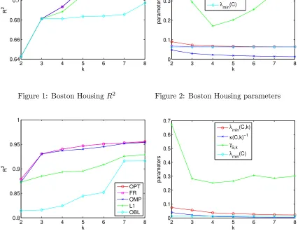
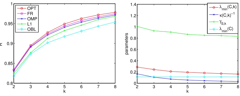
Figures 1, 3 and 5 show the results for the three data sets. The main insight is that on all data sets, Forward Regression performs optimally or near-optimally, and OMP is only slightly worse. This is despite the fact that (as we discuss shortly) the spectral properties would not necessarily predict such near-optimal performance. Lasso performs somewhat worse on all data sets, and, not surprisingly, the baseline oblivious algorithm performs even worse. The last fact implies that the optimal solution is non-trivial in that it must account for correlation between the observation variables. The order of performance of the greedy algorithms match the order of the strength of the theoretical bounds we derived for them.
On the World Bank data (Figure 3), all algorithms perform quite well with just 2–3 features already. The main reason is that adolescent birth rate is by itself highly predictive of life expectancy, so the first feature selected by all algorithms already contributes highR2
value.
Figures 2, 4 and 6 show the different spectral quantities for the data sets, for varying values ofk. Both of the real-world data sets are nearly singular, as evidenced by the small
λmin(C) values. In fact, the near-singularities manifest themselves for small values of k
already; in particular, since λmin(C,2) is already small, we observe that there are pairs of
highly correlated observations variables in the data sets. Thus, the bounds on approximation we would obtain by considering merely λmin(C, k) or λmin(C,2k) would be quite weak.
Notice, however, that they are still quite a bit stronger than the inverse condition number
κ(C, k)−1: this bound — which is closely related to the RIP property frequently at the center of sparse approximation analysis — takes on much smaller values, and thus would be an even looser bound than the eigenvalues.
On the other hand, the submodularity ratiosγSFR,k for all the data sets are much larger
than the other spectral quantities (almost 5 times larger, on average, than the corresponding
2 3 4 5 6 7 8 0.64
0.66 0.68 0.7 0.72 0.74
k
R
2
OPT FR OMP L1 OBL
Figure 1: Boston HousingR2
2 3 4 5 6 7 8
0 0.1 0.2 0.3 0.4 0.5
k
parameters
λ
min(C,k)
λ
min(C,2k)
κ(C,k)−1
γ
S,k
λ
min(C)
Figure 2: Boston Housing parameters
2 3 4 5 6 7 8
0.8 0.85 0.9 0.95 1
k
R
2
OPT FR OMP L1 OBL
Figure 3: World Bank R2
2 3 4 5 6 7 8
0 0.1 0.2 0.3 0.4 0.5 0.6 0.7
k
parameters
λmin(C,k)
κ(C,k)−1
γ
S,k
λmin(C)
Figure 4: World Bank parameters
monotonically decreasing in k— this is due to the dependency of γSFR,k on the set SFR,
which is different for everyk.
The discrepancy between the small values of the eigenvalues and the good performance of all algorithms shows that bounds based solely on eigenvalues can sometimes be loose. Significantly better bounds are obtained from the submodularity ratioγSFR,k , which takes
on values above 0.2, and significantly larger in many cases. While not entirely sufficient to explain the performance of the greedy algorithms, it shows that the near-singularities of C do not align unfavorably with b, and thus do not provide an opportunity for strong supermodular behavior that adversely affects greedy algorithms.
The synthetic data set we generated is somewhat further from singular, with λmin(C)≈